Intelligent Distributed Swarm Control for Large-Scale Multi-UAV Systems: A Hierarchical Learning Approach

Abstract

In this paper, a distributed swarm control problem is studied for large-scale multi-agent systems (LS-MASs). Different than classical multi-agent systems, an LS-MAS brings new challenges to control design due to its large number of agents. It might be more difficult for developing the appropriate control to achieve complicated missions such as collective swarming. To address these challenges, a novel mixed game theory is developed with a hierarchical learning algorithm. In the mixed game, the LS-MAS is represented as a multi-group, large-scale leader–follower system. Then, a cooperative game is used to formulate the distributed swarm control for multi-group leaders, and a Stackelberg game is utilized to couple the leaders and their large-scale followers effectively. Using the interaction between leaders and followers, the mean field game is used to continue the collective swarm behavior from leaders to followers smoothly without raising the computational complexity or communication traffic. Moreover, a hierarchical learning algorithm is designed to learn the intelligent optimal distributed swarm control for multi-group leader–follower systems. Specifically, a multi-agent actor–critic algorithm is developed for obtaining the distributed optimal swarm control for multi-group leaders first. Furthermore, an actor–critic–mass method is designed to find the decentralized swarm control for large-scale followers. Eventually, a series of numerical simulations and a Lyapunov stability proof of the closed-loop system are conducted to demonstrate the performance of the developed scheme.

1. Introduction

The concept of swarming in multi-agent systems (MASs) has been adopted from the biological swarming behavior in nature ranging from bacteria to more advanced mammals [1]. Examples of swarming behavior include flock of birds [2], school of fish [3], and cooperation of ants [4], which form groups of MASs to achieve certain tasks such as threatening predators, foraging food, and energy-efficient flying during migration. Over the past few decades, the biological swarm system has been widely adopted by researchers [5,6,7,8,9,10,11,12,13]. A survey of the recent development in the control and optimization of swarm systems was presented in [14]. Aside from that, the cooperative control problem for the swarming system was studied in [15]. Skobelev et al. [16] proposed a prototype system using a swarm of unmanned aerial vehicles (UAVs), which includes coordinated flight plans with reconfiguration in the presence of disruptive events. In [17], a new formation control scheme with smooth distributed consensus control for multi-UAV systems was developed. The authors in [18] proposed intelligent flight decision techniques for UAVs for cooperative target tracking using an end-to-end, cooperative, multi-agent reinforcement learning scheme. Zhao et al. [19] developed a flocking obstacle avoidance algorithm with shared obstacle information. Despite all of these recent efforts, the traditional cooperative control of large-scale multi-agent systems (LS-MASs) suffers from the well-known “Curse of Dimensionality” [20] and communication reliability [21] problem.

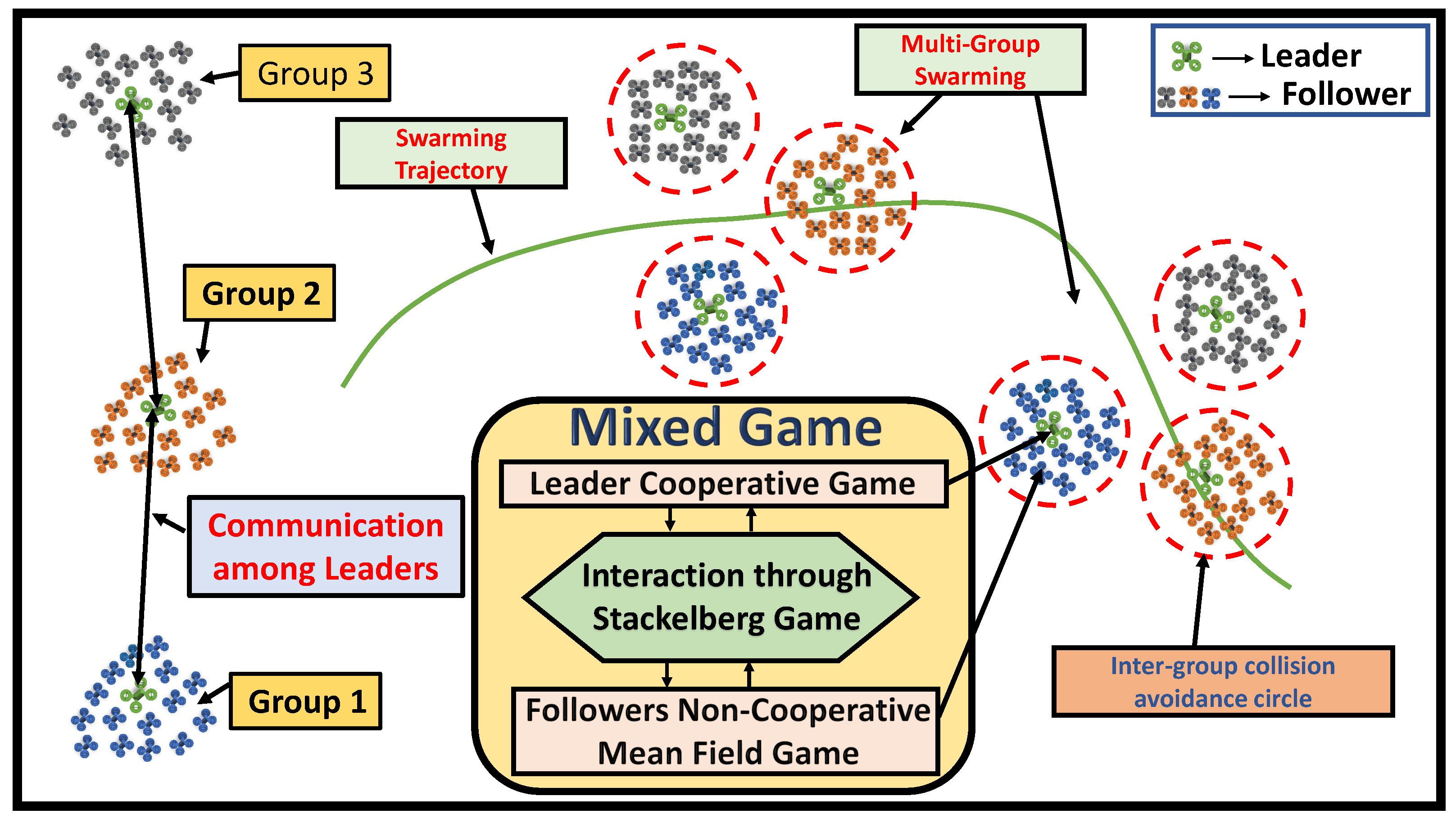
To address these challenges, a mixed game theory is proposed and utilized to formulate the optimal swarming problem for large scale multi-agent systems. The overall structure of the developed mixed game theoretical swarming is shown in Figure 1. First, the LS-MAS is reformulated as a multi-group large-scale leader–follower system by dividing a large number of agents into several subgroups with a leader and a large number of followers in each group. The objective of each group is to achieve optimal distributed swarming behavior. To achieve desired swarming, a mixed game theory was developed by seamlessly integrating (1) the cooperative game [22,23] to ensure the collective swarming behavior among multi-group leaders, where the leaders from each group cooperate with other leaders to maintain the overall multi-group swarming while avoiding inter-group collision, (2) the Stackelberg game [24,25] to connect the leader with its corresponding followers, where a set of coupling functions is introduced by the Stackelberg game in order to maintain leader–follower cohesion in each group, which guarantees that the followers from each group successfully achieve the swarming behavior of their respective leaders, and (3) the mean field game (MFG) [26,27,28] between non-cooperative followers used to continue the collective swarming behavior from the leaders to large-scale followers. The MFG deal involves the “Curse of Dimensionality” and the communication complexity problem of a traditional cooperative game. A probability density function (PDF) (i.e., mass) is employed in the MFG to replace the large number of agents’ state information. Since the mass function has the same dimension as the state space, it eliminates the correlation between rising computing complexity and the agents’ increasing population by reducing the dimension of the cost function.

However, to obtain the mass function, a new partial differential equation (PDE) (i.e., the Fokker–Planck–Kolmogorov (FPK) [29] equation), is adopted. Then, the optimal decentralized swarming control for large-scale followers in each group can be obtained by solving coupled Hamiltonian–Jacobi–Bellman (HJB) and FPK equations [30]. Meanwhile, the distributed optimal swarming control for multi-group leaders can be solved by using the multi-player cooperative HJB equation. However, it is very difficult and even impossible to solve those PDEs in real time due to its complexity and coupling. Hence, adaptive dynamic programming [31] and a reinforcement learning [32] algorithm were adopted. Specifically, a hierarchical learning structure was developed to obtain the optimal swarming control for the multi-group leader–follower system. This includes (1) multi-agent actor–critic-based distributed optimal swarm control for multi-group leaders and (2) actor–critic-mass (ACM)-based decentralized swarm control for large-scale followers. In ACM learning-based control, the actor neural network (NN) is used to approximate the optimal decentralized control, the critic NN is used for approximating the optimal evaluation function, and the mass NN approximates the FPK solution. The main contributions of the article are as follows:

• A novel mixed game theory is developed with cooperative leaders and non-cooperative followers in order to achieve multi-group optimal swarming control which addresses the challenge of the curse of dimensionality and unrealistic communication.
• A hierarchical learning structure with actor–critic-based, leader-distributed swarming and actor–critic–mass-based, large-scale followers decentralized swarming is implemented in real time to learn the solution of the overall intelligent optimal swarming control.

The structure of this paper is as follows. Section 2 provides the significance of the developed algorithm, and Section 3 includes the problem formulation. In Section 4, the novel mixed game hierarchical learning-based intelligent optimal swarming control scheme is developed. Then, the numerical simulation is shown in Section 5 to demonstrate the effectiveness of the proposed design.

2. Significance of Mixed Game Theory-Based Intelligent Distributed Swarm Control

The traditional cooperative control [33,34,35] of multi-agent systems requires communication among all agents to achieve optimal control, which encounters issues with significant computational complexity and the requirement of low-latency communication in real time. In particular, when a swarm contains a massive population which is known as an LS-MAS, it suffers from the following challenges: (1) a high-quality communication network is required for exchanging information in an LS-MAS to achieve the conventional cooperative swarming behavior, although in practice, maintaining these communication networks is unrealistic, and (2) each agent must be aware of the states of the other agents to accomplish the desired multi-group swarming behavior. As the number of agents increases, the computational complexity problem increases substantially, which brings about the well-known “Curse of Dimensionality” [20] problem. Aside from that, most of the existing studies focus on the swarming behavior of single-group MASs with a limited number of agents while avoiding multi-group large-scale MASs, whose examples in a practical environment are ubiquitous. For instance, dividing an MAS into multiple groups can help it effectively handle multi-task missions, whereas a single group cannot, such as in predator formation during multi-prey hunting or cooperative searching for multiple objectives. Recently, several studies in MASs addressed this issue to some extent. Zhang et al. [36] developed a type of multi-group formation tracking control, where the agents are divided into several subgroups to form different desired sub-formations. A distributed impulsive control method with and without the input delay for multi-group formation tracking control was presented in [37]. Moreover, collision avoidance among multi-group UAVs was studied in [38]. In this paper, the developed mixed game theory-based distributed control addressed the challenges of the existing single-group traditional multi-agent cooperative control. At first, the large-scale multi-agent system is divided into multiple groups. Then, each group is reformulated with a leader and a large number of followers. The leader from each group plays the cooperative game to achieve the optimal swarming behavior for all the agents and ensure collision avoidance between the group of agents. The leader just needs to know the PDF information of the followers’ group instead of knowing the state information of each follower. This reduces the dimension of the cost function significantly. However, the leaders still need to exchange the state information with other group leaders. The communication cost of exchanging information is still low compared with a large number of agents, as the agents are divided into a few of subgroups. On the other hand, this upper-level communication between leaders significantly ensures the optimal swarming behavior and collision avoidance of the group of agents. In addition, the followers from each group are guided by their respective leaders and play a non-cooperative game inside the group to reduce the computational complexity and communication problem significantly. To validate the effectiveness of the developed algorithm, the performance of the developed method is further compared against the existing traditional cooperative control method in the simulation (Section 5.2).

3. Problem Formulation

Consider an LS-MAS being reformulated as a multi-group large-scale leader–follower system, with each group having a leader with a large number of followers. Then, assume there are M groups with M leaders as well as $N_F^i$ being the number of followers in the ith group. Next, the dynamics of the leader and follower q in group i are defined as follows.

Leader:

$$d{x}_L^i=[F_a\left(x_L^i\right)+G_a\left(x_L^i\right)u_L^i]dt+\sqrt{2{\nu }^i}d{\omega }_L^i$$

(1)

where $x_L^i\in {\mathbb{R}}^m$ denotes the system state and $u_L^i\in {\mathbb{R}}^n$ denotes the control input. Moreover, ${\omega }_L^i\in {\mathbb{R}}^m$ denotes independent wiener processes which represents the environmental noise, and ${\nu }^i$ is a non-negative parameter. The functions $F_a(.)$ and $G_a(.)$ represent the intrinsic dynamics of the leaders.

Follower:

$$d{x}_{F,q}^i=[F_s\left(x_{F,q}^i\right)+G_s\left(x_{F,q}^i\right)u_{F,q}^i]dt+\sqrt{2{\nu }^i}{\omega }_{F,q}^i$$

(2)

where $x_{F,q}^i\in {\mathbb{R}}^m$ is the state and $u_{F,q}^i\in {\mathbb{R}}^n$ is the control input of the follower q. Moreover, ${\omega }_{F,q}^i\in {\mathbb{R}}^m$ denotes the wiener process. The functions $F_s(.)$ and $G_s(.)$ represent the intrinsic dynamics of the followers.

3.1. Multi-Group Optimal Swarming Control Formulation

In this section, the mixed game theory is designed to formulate the optimal swarming control for multi-group large-scale leader–follower systems. Next, the details of the developed scheme are given as follows:

Collective Swarming among Multi-Group Leaders: To achieve the collective swarming behavior for all groups in the system, a predefined reference trajectory $x_d\left(t\right)\in {\mathbb{R}}^m$ is given to all leaders ahead of the mission. Next, the desired formation vector with respect to the reference trajectory for a group’s ith leader can be denoted as ${\lambda }_L^i\in {\mathbb{R}}^m$. Then, the desired trajectory for the leader in group i is defined as follows:

$$x_{L,d}^i\left(t\right)=x_d\left(t\right)+{\lambda }_L^i$$

(3)

Then, the tracking error of the leader i is defined as $e_L^i\left(t\right)=x_L^i\left(t\right)-x_{L,d}^i\left(t\right)$ with the tracking error dynamic as follows:

$$\begin{array}{cc}\hfill d{e}_L^i& =d{x}_L^i-d{x}_{L,d}^i\hfill \\ \hfill & =[F_{ar}\left(e_L^i\right)+G_{ar}\left(e_L^i\right)u_L^i]dt+\sqrt{2{\nu }^i}d{\omega }_L^i\hfill \end{array}$$

(4)

where $F_{ar}\left(e_L^i\right)=F_a(e_L^i+x_{L,d}^i)-(d{x}_{L,d}^i/dt)$ and $G_{ar}\left(e_L^i\right)=G_a(e_L^i+x_{L,d}^i)$. Additionally, the tracking error function for the leader in group i is given as

$${\Phi }_{\mathrm{SE},\mathrm{L}}\left(x_L^i\right)={\parallel x_L^i-x_{L,d}^i\parallel }_{Q_{\mathrm{SE},\mathrm{L}}}^2$$

(5)

where $Q_{\mathrm{SE},\mathrm{L}}$ is a matrix. To achieve the common goal for all groups (i.e., the collective swarming behavior), each leader needs to communicate with the leaders in the neighborhood groups to avoid inter-group collisions. Let $\mathcal{G}=\{\mathcal{A},\mathcal{V},\mathcal{E}\}$ is a graph that describes the connection among the leaders of M groups, with $\mathcal{A}=\left[a_{ij}\right]\in {\mathbb{R}}^{M\times M}$ is an adjacency matrix (i.e., ${\mathcal{A}}^T=\mathcal{A}$). In addition, $\mathcal{V}\left(\mathcal{G}\right)=\{1,2,...,M\}$ denotes the set of leader vertices, and $\mathcal{E}\in \mathcal{V}\times \mathcal{V}$ is the set of edges. The element $a_{ij}$ of the adjacency matrix is defined as $a_{ij}=a_{ji}=1$ if $(i,j)\in \mathcal{E}$ (i.e., the leaders of group i and j are connected); otherwise, $a_{ij}=a_{ji}=0$. Moreover, we assume that $a_{ii}=0$. To define the neighborhood of each leader, sensing and communicating distance is needed. Let $h>0$ denote the communicating distance. Then, the neighborhood set ${\mathcal{M}}_L^i$ of the leader of group i is defined as follows:

$${\mathcal{M}}_L^i\left(t\right)=\{j\in \mathcal{V}:\parallel x_L^i\left(t\right)-x_L^j\left(t\right){\parallel }_{Q_1}^2<h,j\ne i\}$$

(6)

where $Q_1$ is a positive definite matrix. Additionally, the communication between group leader i and j can be possible if $j\in {\mathcal{M}}_L^i\left(t\right)$. Furthermore, collision avoidance between leaders and their respective followers needs to be addressed for multi-group leader–follower swarming control in order to ensure safe path planning and guide the group to their desired swarming movement. The cost function for collision among leaders is

$$\begin{array}{cc}\hfill & {\Phi }_{\mathrm{CA},\mathrm{L}}(x_L^i,x_L^{-i})=w_{\mathrm{CA},\mathrm{L}}\sum _{j\in {\mathcal{M}}_L^i}{a}_{i,j}{\left[\begin{array}{c}\exp \{\parallel x_L^i-x_L^j{\parallel }_{Q_{\mathrm{CA},\mathrm{L}}}^2-d_L^{i,j}\}-1\end{array}\right]}^{-1}\hfill \end{array}$$

(7)

where $Q_{\mathrm{CA},\mathrm{L}}$ is a weighting matrix, $w_{\mathrm{CA},\mathrm{L}}$ is a weighting parameter, and $x_L^{-i}={\left\{x_L^j\right\}}_{j\in {\mathcal{M}}_L^i}$. In addition, $d_L^{i,j}$ is the separating distance between leaders i and j, which is chosen so that it always ensures the avoidance of collision between two groups (i.e., collisions between any two leaders and their corresponding followers). Moreover, to achieve collective swarming behavior while avoiding group collision, the cohesion between the leader and large-scale followers needs to be maintained. In this regard, the leader–follower coupling function is introduced as follows.

Leader–Follower Coupling Functions for Swarming: To achieve a group swarming behavior, a set of coupling functions is defined by the Stackelberg game ([24]). The coupling function that forces the leader to keep cohesion with their corresponding followers is defined as follows:

$$\begin{array}{c}\hfill {\Phi }_{\mathrm{CP},\mathrm{L}}(x_L^i,{\rho }^i)=w_{\mathrm{CP},\mathrm{L}}{\parallel x_L^i-\mathbb{E}\left\{x_F^i\right\}\parallel }_{Q_{\mathrm{CP},\mathrm{L}}}^2\end{array}$$

(8)

where ${\rho }^i(x_F^i,t)$ is the probability density function (PDF) of the large-scale followers’ state in the ith group, $\mathbb{E}\left\{x_F^i\right\}$ is the expected value, and $w_{\mathrm{CP},\mathrm{L}}$ and $Q_{\mathrm{CP},\mathrm{L}}$ are the weighting matrix and weighting parameter, respectively. Now, the leader–follower swarming coupling function is

$$\begin{array}{c}\hfill {\Phi }_{\mathrm{CP},\mathrm{F}}(x_{F,q}^i,x_L^i)=w_{\mathrm{CP},\mathrm{F}}{\left[\begin{array}{c}\exp \{r^i-\parallel x_{F,q}^i-x_L^i{\parallel }_{Q_{\mathrm{CP},\mathrm{F}}}^2\}-1\end{array}\right]}^{-1}\end{array}$$

(9)

where $Q_{\mathrm{CP},\mathrm{F}}$ is a weighting matrix, $w_{\mathrm{CP},\mathrm{F}}$ is a weighting parameter, and $r^i$ is the maximum safe distance of the ith group’s followers. This distance $r^i$ ensures inter-group collision avoidance by keeping the followers within the safe distance limit.

Leader–Follower Coupling Functions for Swarming: The followers from each group track their respective leaders in order to achieve the group swarming behavior. The tracking error of the follower q in group i is derived as $e_{F,q}^i\left(t\right)=x_{F,q}^i\left(t\right)-x_L^i\left(t\right)$, with the tracking error dynamics

$$\begin{array}{c}\hfill d{e}_{F,q}^i=\left[F_{sr}\left(e_{F,q}^i\right)+G_{sr}\left(e_{F,q}^i\right)u_{F,q}^i\right]dt+\sqrt{2{\nu }^i}d{\omega }_{F,q}^i\end{array}$$

(10)

where

$$\begin{array}{cc}\hfill F_{sr}\left(e_{F,q}^i\right)& =F_s(e_{F,q}^i+x_L^i)-F_a\left(x_L^i\right);G_{sr}\left(e_{F,q}^i\right)=G_s(e_{F,q}^i+x_L^i)-G_a\left(x_L^i\right)\frac{u_L^i}{u_{F,q}^i}\hfill \end{array}$$

Now, the followers’ tracking error cost function can be derived as follows:

$${\Phi }_{\mathrm{SE},\mathrm{F}}\left(x_{F,q}^i\right)={\parallel x_{F,q}^i-x_L^i\parallel }_{Q_{\mathrm{SE},\mathrm{F}}}^2$$

(11)

where $Q_{\mathrm{SE},\mathrm{F}}$ is a positive definite matrix. Then, the same group large scale follower collision avoidance function is as follows:

$${\Phi }_{\mathrm{CA},\mathrm{F}}(x_{F,q}^i,{\rho }^i)=w_{\mathrm{CA},\mathrm{F}}{\int }_{x_F^i}\frac{{\rho }^i(x_F^i,t)}{[{\epsilon }^2+\parallel x_{F,q}^i-\mathbb{E}\left\{x_F^i\right\}{{\parallel }_{Q_{\mathrm{CA},\mathrm{F}}}^2]}^{\beta }}d{x}_F^i$$

(12)

where $Q_{\mathrm{CA},\mathrm{F}}$ and $w_{\mathrm{CA},\mathrm{F}}$ are the weighting matrix and weighting parameter, respectively. Moreover, $\epsilon$ and $\beta$ are positive constants. Furthermore, the cohesion function of the followers with their respective group center can be derived as follows:

$$\begin{array}{c}\hfill {\Phi }_{\mathrm{C},\mathrm{F}}(x_{F,q}^i,{\rho }^i)=w_{\mathrm{C},\mathrm{F}}\left\{\parallel x_{F,q}^i-\mathbb{E}\left\{x_F^i\right\}{\parallel }_{Q_{\mathrm{C},\mathrm{F}}}^2\right\}\end{array}$$

(13)

with the weighting matrix $Q_{\mathrm{C},\mathrm{F}}$ and weighting parameter $w_{\mathrm{C},\mathrm{F}}$. This function helps each follower from the same group to stay close to the other members of the group.

Overall Optimal Swarming Control for Multi-Group LS-MAS: The goal of the leaders is to achieve overall swarming control by minimizing the following cost function.

Leader:

$$\begin{array}{cc}\hfill & V_L(x_L,\rho )=\sum _{i=1}^M{V}_L^i(x_L^i,x_L^{-i},{\rho }^i)=\sum _{i=1}^M\mathbb{E}\left\{{\int }_0^{\infty }\left[\begin{array}{c}{\Phi }_{\mathrm{L}}(x_L^i,x_L^{-i},u_L^i)+{\Phi }_{\mathrm{CP},\mathrm{L}}(x_L^i,{\rho }^i)\end{array}\right]dt\right\}\hfill \end{array}$$

(14)

where ${\Phi }_{\mathrm{L}}(x_L^i,x_L^{-i},u_L^i)={\Phi }_{\mathrm{SE},\mathrm{L}}\left(x_L^i\right)+{\Phi }_{\mathrm{CA},\mathrm{L}}(x_L^i,x_L^{-i})+{\parallel u_L^i\parallel }_{R_L^i}^2$, $V_L^i$ is the cost function of the ith group leader and $R_L^i$ is the positive weight matrix. The functions ${\Phi }_{\mathrm{SE},\mathrm{L}}\left(x_L^i\right)$, ${\Phi }_{\mathrm{CA},\mathrm{L}}(x_L^i,x_L^{-i})$, and ${\Phi }_{\mathrm{CP},\mathrm{L}}(x_L^i,{\rho }^i)$ derived in Equations (5), (7), and (8) are the tracking error, collision avoidance, and coupling function of the leader, respectively. Moreover, the objective of the follower q in the group i is to minimize the following cost function to achieve the group swarming behavior.

Follower:

$$\begin{array}{cc}\hfill V_{F,q}^i(x_{F,q}^i,x_L^i,{\rho }^i)& =\mathbb{E}\left\{{\int }_0^{\infty }\left[\begin{array}{c}{\Phi }_{\mathrm{F}}(x_{F,q}^i,x_L^i,u_{F,q}^i)+{\Phi }_{\mathrm{CA},\mathrm{F}}(x_{F,q}^i,{\rho }^i)+{\Phi }_{\mathrm{C},\mathrm{F}}(x_{F,q}^i,{\rho }^i)\end{array}\right]dt\right\}\hfill \\ \hfill & \mathrm{s}.\mathrm{t}.\parallel x_{F,q}^{i,o}-x_L^i\parallel <r^i\hfill \end{array}$$

(15)

where ${\Phi }_{\mathrm{F}}(x_{F,q}^i,x_L^i,u_{F,q}^i)={\Phi }_{\mathrm{SE},\mathrm{F}}\left(x_{F,q}^i\right)+{\Phi }_{\mathrm{CP},\mathrm{F}}(x_{F,q}^i,x_L^i)+{\parallel u_{F,q}^i\parallel }_{R_{F,q}^i}^2$, $R_{F,q}^i$ is the positive weight matrix and $x_{F,q}^{i,o}$ is the initial state of the follower q. The functions ${\Phi }_{\mathrm{SE},\mathrm{F}}\left(x_{F,q}^i\right)$, ${\Phi }_{\mathrm{CP},\mathrm{F}}(x_{F,q}^i,x_L^i)$, ${\Phi }_{\mathrm{C},\mathrm{F}}(x_{F,q}^i,{\rho }^i)$, and ${\Phi }_{\mathrm{CA},\mathrm{F}}(x_{F,q}^i,{\rho }^i)$ derived in Equations (9) and (11)–(13) are the follower tracking error, coupling, cohesion, and collision avoidance functions, respectively. Here, the initial states of the followers from all groups are subject to a constraint in order to keep the followers inside a specific region defined by the distance $r^i$. This distance is the radius of an enclosing circle which acts as a collision-avoiding region for the respective groups.

3.2. Mixed Game Theory-Based Multi-Group, Large-Scale Leader–Follower-Distributed Optimal Swarming Control

To achieve the overall swarming behavior for all groups, the overall cost function of the leaders’ (Equation (14)) and followers’ individual cost function (Equation (15)) need to be minimized. Now, the leader-follower Hamiltonian can be obtained using Bellman’s principle of optimality [39] and optimal control [20]. The Hamiltonian of all the leaders is as follows:

$$\begin{array}{cc}\hfill & H_L[x_L,{\partial }_{x_L}{V}_L(x_L,\rho )]=\sum _{i=1}^M{H}_L^i[x_L^i,{\partial }_{x_L^i}{V}_L^i(x_L^i,x_L^{-i},{\rho }^i)]\hfill \end{array}$$

(16)

with individual leaders distributed Hamiltonian:

$$\begin{array}{cc}\hfill & H_L^i[x_L^i,{\partial }_{x_L^i}{V}_L^i(x_L^i,x_L^{-i},{\rho }^i)]=\mathbb{E}\left\{\left[\begin{array}{c}{\Phi }_{\mathrm{L}}(x_L^i,x_L^{-i},u_L^i)+{\Phi }_{\mathrm{CP},\mathrm{L}}(x_L^i,{\rho }^i)+{\partial }_{x_L^i}{V_L^i}^T\\ (x_L^i,x_L^{-i},{\rho }^i)[F_a\left(x_L^i\right)+G_a\left(x_L^i\right)u_L^i]\end{array}\right]\right\}\hfill \end{array}$$

(17)

The Hamiltonian for the follower q from the ith group is derived as follows:

$$\begin{array}{cc}\hfill & H_{F,q}^i[x_{F,q}^i,{\partial }_{x_{F,q}^i}{V}_{F,q}^i(x_{F,q}^i,x_L^i,{\rho }^i)]=\mathbb{E}\left\{\left[\begin{array}{c}{\Phi }_{\mathrm{F}}(x_{F,q}^i,x_L^i,u_{F,q}^i)+{\Phi }_{\mathrm{CA},\mathrm{F}}(x_{F,q}^i,{\rho }^i)+{\Phi }_{\mathrm{C},\mathrm{F}}(x_{F,q}^i,{\rho }^i)\\ +{\partial }_{x_{F,q}^i}{V}_{F,q}^{i^T}(x_{F,q}^i,x_L^i,{\rho }^i)+[F_s\left(x_{F,q}^i\right)+G_s\left(x_{F,q}^i\right)u_{F,q}^i]\end{array}\right]\right\}\hfill \end{array}$$

(18)

Now, the multi-group leaders Hamiltonian–Jacobi–Bellman (HJB) equation can be derived from the cooperative game is as follows:

$$\begin{array}{c}\hfill \mathbb{E}\left\{{\Phi }_{\mathrm{CP},\mathrm{L}}(x_L^i,{\rho }^i)\right\}=\mathbb{E}\left\{\left[\begin{array}{c}-{\partial }_t{V}_L^i(x_L^i,x_L^{-i},{\rho }^i)-\sqrt{2{\nu }^i}\Delta V_L^i(x_L^i,x_L^{-i},{\rho }^i)\\ +H_L^i[x_L^i,{\partial }_{x_L^i}{V}_L^i(x_L^i,x_L^{-i},{\rho }^i)]\end{array}\right]\right\}\end{array}$$

(19)

Furthermore, a coupled HJB and Fokker–Planck–Kolmogorov(FPK) equations for the large number of followers, using MFG can be obtained as follows:

Follower (HJB):

$$\begin{array}{c}\hfill \mathbb{E}\left\{{\Phi }_{\mathrm{CA},\mathrm{F}}(x_{F,q}^i,{\rho }^i)+{\Phi }_{\mathrm{C},\mathrm{F}}(x_{F,q}^i,{\rho }^i)\right\}=\mathbb{E}\left\{\left[\begin{array}{c}-{\partial }_t{V}_{F,q}^i(x_{F,q}^i,x_L^i,{\rho }^i)-\sqrt{2{\nu }^i}\Delta V_{F,q}^i(x_{F,q}^i,\\ x_L^i,{\rho }^i)+H_{F,q}^i[x_{F,q}^i,{\partial }_{x_{F,q}^i}{V}_{F,q}^i(x_{F,q}^i,x_L^i,{\rho }^i)]\end{array}\right]\right\}\end{array}$$

(20)

Follower (FPK):

$$\begin{array}{c}\hfill \mathbb{E}\left\{{\partial }_t{\rho }^i(x_{F,q}^i,t)-\sqrt{2{\nu }^i}\Delta {\rho }^i(x_{F,q}^i,t)-div\left({\rho }^i{D}_p{H}_{F,q}^i[x_{F,q}^i,{\partial }_{x_{F,q}^i}{V}_{F,q}^i(x_{F,q}^i,x_L^i,{\rho }^i)]\right)\right\}=0\end{array}$$

(21)

Then, according to optimal control theory, the mixed game-based distributed optimal swarming control for a multi-group leader–follower system can be attained as follows:

Leader:

$$\begin{array}{c}\hfill u_L^i\left(x_L^i\right)=-\frac{1}{2}\mathbb{E}\left\{R_L^{i^{-1}}{G}_a^T\left(x_L^i\right){\partial }_{x_L^i}{V}_L^i(x_L^i,x_L^{-i},{\rho }^i)\right\}\end{array}$$

(22)

Follower:

$$\begin{array}{c}\hfill u_{F,q}^i\left(x_{F,q}^i\right)=-\frac{1}{2}\mathbb{E}\left\{R_{F,q}^{i^{-1}}{G}_s^T\left(x_{F,q}^i\right){\partial }_{x_{F,q}^i}{V}_{F,q}^i(x_{F,q}^i,x_L^i,{\rho }^i)\right\}\end{array}$$

(23)

Remark 1.

The coupled HJB-FPK equations of the follower and the HJB equation for the leader must be solved in real time in order to determine the optimal control policy. The backward HJB and forward FPK equations, however, are coupled multidimensional nonlinear PDEs that are difficult to solve. Therefore, in this paper, a hierarchical learning-based, multi-actor-critic–mass NN is developed to learn the optimal control online.

4. Hierarchical Learning-Based Intelligent Optimal Distributed Swarming Control

4.1. Hierarchical Learning-Based Control for Multi-Group Leader–Follower Systems

In this section, a hierarchical learning-based actor–critic–mass algorithm (see Figure 2) is developed and explained in detail. It includes (1) multi-agent actor–critic neural networks (NNs) to obtain the cooperative game-based distributed optimal swarm control for multi-group leaders and (2) actor–critic–mass-based decentralized control for large-scale followers within the same game to obtain the mean field game-based swarming. Additionally, the Stackelberg game integrates distributed swarming control for leaders and decentralized control for followers into a unified framework and further obtains the overall distributed intelligent swarming control for multi-group leader–follower systems.

Ideal Actor–Critic Set-up for Leaders:

$$\begin{array}{cc}\hfill \mathrm{Critic}:V_L^{i*}(x_L^i,x_L^{-i},{\rho }^i)& =\mathbb{E}\left\{W_{V,L}^{i^T}{\varphi }_{V,L}^i+{\epsilon }_{{\mathrm{HJB}}_{\mathrm{L}}}^i\right\}\hfill \\ \hfill \mathrm{Actor}:u_L^{i*}(x_L^i,x_L^{-i},{\rho }^i)& =\mathbb{E}\left\{W_{u,L}^{i^T}{\varphi }_{u,L}^i+{\epsilon }_{\mathrm{u},\mathrm{L}}^i\right\}\hfill \end{array}$$

(24)

Ideal Actor–Critic–Mass Set-up for Followers:

$$\begin{array}{cc}\hfill \mathrm{Critic}:V_{F,q}^{i*}(x_{F,q}^i,x_L^i,{\rho }^i)& =\mathbb{E}\left\{W_{V,F,q}^{i^T}{\varphi }_{V,F,q}^i+{\epsilon }_{{\mathrm{HJB}}_{\mathrm{F},\mathrm{q}}}^i\right\}\hfill \\ \hfill \mathrm{Actor}:u_{F,q}^{i*}(x_{F,q}^i,x_L^i,{\rho }^i)& =\mathbb{E}\left\{W_{u,F,q}^{i^T}{\varphi }_{u,F,q}^i+{\epsilon }_{\mathrm{u},\mathrm{F},\mathrm{q}}^i\right\}\hfill \\ \hfill \mathrm{Mass}:{\rho }^i(x_{F,q}^i,t)& =\mathbb{E}\left\{W_{\rho ,F,q}^{i^T}{\varphi }_{\rho ,F,q}^i+{\epsilon }_{{\mathrm{FPK}}_{\mathrm{F},\mathrm{q}}}^i\right\}\hfill \end{array}$$

(25)

where $W_{V,L}^i$, $W_{u,L}^i$, $W_{V,F,q}^i$, $W_{u,F,q}^i$, and $W_{\rho ,F,q}^i$ are the respective weights for the leader and follower critic, actor, and mass neural network (NN). Also, $\varphi (.)$ is the activation function and $\epsilon$ is the reconstruction error of the respective neural networks. Then, the estimated cost and control functions of the leader are as follows:

Estimated Actor-Critic for Multi-Group Leaders:

$$\begin{array}{cc}\hfill \mathrm{Critic}:{\widehat{V}}_L^i(x_L^i,x_L^{-i},{\overline{\widehat{\rho }}}^i)& =\mathbb{E}\left\{{{\widehat{W}}_{V,L}}^{i^T}{\widehat{\varphi }}_{V,L}^i\right\}\hfill \\ \hfill \mathrm{Actor}:{\widehat{u}}_L^i(x_L^i,x_L^{-i},{\overline{\widehat{\rho }}}^i)& =\mathbb{E}\left\{{\widehat{W}}_{u,L}^{i^T}{\widehat{\varphi }}_{u,L}^i\right\}\hfill \end{array}$$

(26)

Please be aware that the leader from each group collects the estimated PDF from each decentralized follower in the same group. Then, the leader evaluates the statistic average of the received PDF (i.e., ${\overline{\widehat{\rho }}}^i={\sum }_{F,q}{\widehat{\rho }}_{F,q}^i$). Next, The residual errors that result from substituting the approximation in Equation (26) into Equation (19) can be utilized to adjust the weights of the leader actor and critic neural networks by using the residual errors given as following equations:

$$\begin{array}{c}\hfill \mathbb{E}\left\{e_{{\mathrm{HJB}}_{\mathrm{L}}}^i\right\}=\mathbb{E}\left\{\left[\begin{array}{c}{\Phi }_{\mathrm{CP},\mathrm{L}}(x_L^i,{\overline{\widehat{\rho }}}^i)+{\widehat{W}}_{V,L}^{i^T}[{\partial }_t{\widehat{\varphi }}_{V,L}^i+\sqrt{2{\nu }^i}\Delta {\widehat{\varphi }}_{V,L}^i-{\widehat{H}}_{L,W}^i]\end{array}\right]\right\}\end{array}$$

(27)

$$\begin{array}{c}\hfill \mathbb{E}\left\{e_{\mathrm{u},\mathrm{L}}^i\right\}=\mathbb{E}\left\{{\widehat{W}}_{u,L}^{i^T}{\widehat{\varphi }}_{u,L}^i+\frac{1}{2}{R}_L^{i^{-1}}{G}_a^T\left(x_L^i\right){\partial }_{x_L^i}{\widehat{\varphi }}_{V,L}^i\right\}\end{array}$$

(28)

where the estimated Hamiltonian of the leader ${\widehat{H}}_L^i$ is defined as

$${\widehat{H}}_L^i=H_L^i[x_L^i,{\partial }_{x_L^i}{\widehat{\varphi }}_{V,L}^i]={\widehat{W}}_{V,L}^{i^T}{\widehat{H}}_{L,W}^i$$

Now, let

$$\mathbb{E}\left\{{\Psi }_{V,L}^i(x_L^i,x_L^{-i},{\overline{\widehat{\rho }}}^i)\right\}=\mathbb{E}\left\{{\partial }_t{\widehat{\varphi }}_{V,i}+\sqrt{2{\nu }^i}\Delta {\widehat{\varphi }}_{V,i}-{\widehat{H}}_{L,W}^i\right\}$$

and

$$\mathbb{E}\left\{{\Phi }_{\mathrm{CP},\mathrm{L}}(x_L^i,{\overline{\widehat{\rho }}}^i)\right\}=\mathbb{E}\left\{{\Phi }_{\mathrm{CP},\mathrm{L}}(x_L^i,{\overline{\tilde{\rho }}}^i)+{\Phi }_{\mathrm{CP},\mathrm{L}}(x_L^i,{\rho }^i)\right\}$$

Then, the estimation error from the Equation (27) is therefore rewritten follows:

$$\begin{array}{c}\hfill \mathbb{E}\left\{e_{{\mathrm{HJB}}_{\mathrm{L}}}^i\right\}=\mathbb{E}\left\{\left[\begin{array}{c}{\Phi }_{\mathrm{CP},\mathrm{L}}(x_L^i,{\rho }^i)+{\Phi }_{\mathrm{CP},\mathrm{L}}(x_L^i,{\overline{\tilde{\rho }}}^i)+{\widehat{W}}_{V,L}^{i^T}{\Psi }_{V,L}^i(x_L^i,x_L^{-i},{\overline{\widehat{\rho }}}^i)\end{array}\right]\right\}\end{array}$$

(29)

Next, the effect of the reconstruction error is considered by substituting the optimal function from Equation (24) to the HJB Equation (19):

$$\begin{array}{c}\hfill \mathbb{E}\left\{{\Phi }_{\mathrm{CP},\mathrm{L}}(x_L^i,{\rho }^i)+W_{V,L}^{i^T}{\Psi }_{V,L}^i(x_L^i,x_L^{-i},{\overline{\rho }}^i)+{\epsilon }_{{\mathrm{HJB}}_{\mathrm{L}}}^i\right\}=0\end{array}$$

(30)

By substituting Equation (30) into Equation (29), the following HJB error equation can be obtained with reconstruction error as:

$$\begin{array}{c}\hfill \mathbb{E}\left\{e_{{\mathrm{HJB}}_{\mathrm{L}}}^i\right\}=\mathbb{E}\left\{\left[\begin{array}{c}{\Phi }_{\mathrm{CP},\mathrm{L}}(x_L^i,{\overline{\tilde{\rho }}}^i)-{\tilde{W}}_{V,L}^{i^T}{\widehat{\Psi }}_{V,L}^i(x_L^i,x_L^{-i},{\overline{\widehat{\rho }}}^i)-W_{V,L}^{i^T}{\tilde{\Psi }}_{V,L}^i(x_L^i,x_L^{-i},{\overline{\tilde{\rho }}}^i)-{\epsilon }_{{\mathrm{HJB}}_{\mathrm{L}}}^i\end{array}\right]\right\}\end{array}$$

(31)

Again, the leader actor NN error is as follows:

$$\begin{array}{c}\hfill \mathbb{E}\left\{e_{\mathrm{u},\mathrm{L}}^i\right\}=\mathbb{E}\left\{\left[\begin{array}{c}-{\tilde{W}}_{u,L}^{i^T}{\widehat{\varphi }}_{u,L}^i(x_L^i,x_L^{-i},{\overline{\widehat{\rho }}}^i)-W_{u,L}^{i^T}{\tilde{\varphi }}_{u,L}^i(x_L^i,x_L^{-i},{\overline{\tilde{\rho }}}^i)-\frac{1}{2}{R}_L^{i^{-1}}{G}_a^T\left(x_L^i\right){\partial }_{x_L^i}{\tilde{V}}_L^i-{\epsilon }_{\mathrm{u},\mathrm{L}}^i\end{array}\right]\right\}\end{array}$$

(32)

where ${\tilde{W}}_{V,L}^i=W_{V,L}^i-{\widehat{W}}_{V,L}^i$ and ${\tilde{W}}_{u,L}^i=W_{u,L}^i-{\widehat{W}}_{u,L}^i$. In addition, the approximated functions can be represented as follows:

$$\begin{array}{c}\hfill \mathbb{E}\left\{{\Psi }_{V,L}^i(x_L^i,x_L^{-i},{\overline{\tilde{\rho }}}^i)\right\}=\mathbb{E}\left\{\left[\begin{array}{c}{\Psi }_{V,L}^i(x_L^i,x_L^{-i},{\rho }^i)-{\widehat{\Psi }}_{V,L}^i(x_L^i,x_L^{-i},{\overline{\widehat{\rho }}}^i)\end{array}\right]\right\}\\ \hfill \mathbb{E}\left\{{\tilde{\varphi }}_{u,L}^i(x_L^i,x_L^{-i},{\overline{\tilde{\rho }}}^i)\right\}=\mathbb{E}\left\{\left[\begin{array}{c}{\tilde{\varphi }}_{u,L}^i(x_L^i,x_L^{-i},{\rho }^i)-{\widehat{\varphi }}_{u,L}^i(x_L^i,x_L^{-i},{\overline{\widehat{\rho }}}^i)\end{array}\right]\right\}\end{array}$$

Next, the multi-agent actor–critic NNs for the leader are updated by using residual errors (Equations (31) and (32)) with the gradient descent method as follows.

Actor–Critic Update Laws for Multi-Group Leaders:

$$\begin{array}{c}\hfill \mathbb{E}\left\{{\dot{\widehat{W}}}_{V,L}^i\right\}=\mathbb{E}\left\{-{\alpha }_{V,L}^i\frac{{\widehat{\Psi }}_{V,L}^i(x_L^i,x_L^{-i},{\overline{\widehat{\rho }}}^i)e_{{\mathrm{HJB}}_{\mathrm{L}}}^{i^T}}{1+\parallel {\widehat{\Psi }}_{V,L}^i(x_L^i,x_L^{-i},{\overline{\widehat{\rho }}}^i){)\parallel }^2}\right\}\end{array}$$

(33)

$$\begin{array}{c}\hfill \mathbb{E}\left\{{\dot{\widehat{W}}}_{u,L}^i\right\}=\mathbb{E}\left\{-{\alpha }_{u,L}^i\frac{{\widehat{\varphi }}_{u,L}^i(x_L^i,x_L^{-i},{\overline{\widehat{\rho }}}^i)e_{\mathrm{u},\mathrm{L}}^{i^T}}{1+\parallel {\widehat{\varphi }}_{u,L}^i(x_L^i,x_L^{-i},{\overline{\widehat{\rho }}}^i){\parallel }^2}\right\}\end{array}$$

(34)

Next, the decentralized optimal swarming control for large-scale followers is as follows.

Estimated Actor–Critic Mass for Followers in the Same Group:

$$\begin{array}{cc}\hfill \mathrm{Critic}:{\widehat{V}}_{F,q}^i(x_{F,q}^i,x_L^i,{\widehat{\rho }}_{F,q}^i)& =\mathbb{E}\left\{{\widehat{W}}_{V,F,q}^{i^T}{\widehat{\varphi }}_{V,F,q}^i\right\}\hfill \\ \hfill \mathrm{Actor}:{\widehat{u}}_{F,q}^i(x_{F,q}^i,x_L^i,{\widehat{\rho }}_{F,q}^i)& =\mathbb{E}\left\{{\widehat{W}}_{u,F,q}^{i^T}{\widehat{\varphi }}_{u,F,q}^i\right\}\hfill \\ \hfill \mathrm{Mass}:{\widehat{\rho }}_{F,q}^i(x_{F,q}^i,t)& =\mathbb{E}\left\{{\widehat{W}}_{\rho ,F,q}^{i^T}{\widehat{\varphi }}_{\rho ,F,q}^i\right\}\hfill \end{array}$$

(35)

The residual error after the substitution of (35) into the HJB and FPK equations (Equations (20) and (21)):

$$\begin{array}{c}\hfill \mathbb{E}\left\{e_{{\mathrm{HJB}}_{\mathrm{F},\mathrm{q}}}^i\right\}=\mathbb{E}\left\{\left[\begin{array}{c}{\Phi }_{\mathrm{CA},\mathrm{F}}(x_{F,q}^i,{\widehat{\rho }}_{F,q}^i)+{\Phi }_{\mathrm{C},\mathrm{F}}(x_{F,q}^i,{\widehat{\rho }}_{F,q}^i)+{\widehat{W}}_{V,F,q}^{i^T}\\ {\partial }_t{\widehat{\varphi }}_{V,F,q}^i+\sqrt{2{\nu }^i}\Delta {\widehat{\varphi }}_{V,F,q}^i-{\widehat{H}}_{F,q,W}^i]\end{array}\right]\right\}\end{array}$$

(36)

$$\begin{array}{c}\hfill \mathbb{E}\left\{e_{\mathrm{u},\mathrm{F},\mathrm{q}}^i\right\}=\mathbb{E}\left\{\left[\begin{array}{c}{\widehat{W}}_{u,F,q}^{i^T}{\widehat{\varphi }}_{u,F,q}^i+\frac{1}{2}{R}_{F,q}^{i^{-1}}{G}_s^T\left(x_{F,q}^i\right){\partial }_{x_{F,q}^i}{\widehat{\varphi }}_{V,F,q}^i\end{array}\right]\right\}\end{array}$$

(37)

$$\begin{array}{c}\hfill \mathbb{E}\left\{e_{{\mathrm{FPK}}_{\mathrm{F},\mathrm{q}}}^i\right\}=\mathbb{E}\left\{{\widehat{W}}_{\rho ,F,q}^{i^T}\left[\begin{array}{c}{\partial }_t{\widehat{\varphi }}_{\rho ,F,q}^i-\sqrt{2{\nu }^i}\Delta {\widehat{\varphi }}_{\rho ,F,q}^i-div\left({\widehat{\varphi }}_{\rho ,F,q}^i\right)D_p{\widehat{H}}_{F,q}^i\end{array}\right]\right\}\end{array}$$

(38)

where

$${\widehat{H}}_{F,q}^i=H_{F,q}^i[x_{F,q}^i,{\partial }_{x_{F,q}^i}{\widehat{\varphi }}_{V,F,q}^i]={\widehat{W}}_{V,F,q}^{i^T}{\widehat{H}}_{F,q,W}^i$$

Again, let

$$\begin{array}{cc}\hfill \mathbb{E}\left\{{\Psi }_{V,F,q}^i(x_{F,q}^i,x_L^i,{\widehat{\rho }}_{F,q}^i)\right\}& =\mathbb{E}\left\{\left[\begin{array}{c}{\partial }_t{\widehat{\varphi }}_{V,F,q}^i+\sqrt{2{\nu }^i}-\Delta {\widehat{\varphi }}_{V,F,q}^i{\widehat{H}}_{F,q,W}^i\end{array}\right]\right\}\hfill \\ \hfill \mathbb{E}\left\{{\Psi }_{\rho ,F,q}^i(x_{F,q}^i,{\widehat{V}}_{F,q}^i,t)\right\}& =\mathbb{E}\left\{\left[\begin{array}{c}{\partial }_t{\widehat{\varphi }}_{\rho ,F,q}^i-\sqrt{2{\nu }^i}\Delta {\widehat{\varphi }}_{\rho ,F,q}^i-div\left({\widehat{\varphi }}_{\rho ,F,q}^i\right)D_p{\widehat{H}}_{F,q}^i\end{array}\right]\right\}\hfill \\ \hfill \mathbb{E}\left\{{\Phi }_{\mathrm{CA},\mathrm{F}}(x_{F,q}^i,{\tilde{\rho }}_{F,q}^i)\right\}& =\mathbb{E}\left\{\left[\begin{array}{c}{\Phi }_{\mathrm{CA},\mathrm{F}}(x_{F,q}^i,{\rho }_{F,q}^i)-{\Phi }_{\mathrm{CA},\mathrm{F}}(x_{F,q}^i,{\widehat{\rho }}_{F,q}^i)\end{array}\right]\right\}\hfill \\ \hfill \mathbb{E}\left\{{\Phi }_{\mathrm{C},\mathrm{F}}(x_{F,q}^i,{\tilde{\rho }}_{F,q}^i)\right\}& =\mathbb{E}\left\{\left[\begin{array}{c}{\Phi }_{\mathrm{C},\mathrm{F}}(x_{F,q}^i,{\rho }_{F,q}^i)-{\Phi }_{\mathrm{C},\mathrm{F}}(x_{F,q}^i,{\widehat{\rho }}_{F,q}^i)\end{array}\right]\right\}\hfill \end{array}$$

The estimation errors in Equations (36) and (38) can be simplified as follows:

$$\begin{array}{c}\hfill \mathbb{E}\left\{e_{{\mathrm{HJB}}_{\mathrm{F},\mathrm{q}}}^i\right\}=\mathbb{E}\left\{\left[\begin{array}{c}{\Phi }_{\mathrm{CA},\mathrm{F}}(x_{F,q}^i,{\rho }_{F,q}^i)+{\Phi }_{\mathrm{CA},\mathrm{F}}(x_{F,q}^i,{\tilde{\rho }}_{F,q}^i)+{\Phi }_{\mathrm{C},\mathrm{F}}(x_{F,q}^i,{\rho }_{F,q}^i)\\ +{\Phi }_{\mathrm{C},\mathrm{F}}(x_{F,q}^i,{\tilde{\rho }}_{F,q}^i)+{\widehat{W}}_{V,F,q}^{i^T}{\Psi }_{V,F,q}^i(x_{F,q}^i,x_L^i,{\widehat{\rho }}_{F,q}^i)\end{array}\right]\right\}\end{array}$$

(39)

$$\begin{array}{c}\hfill \mathbb{E}\left\{e_{{\mathrm{FPK}}_{\mathrm{F},\mathrm{q}}}^i\right\}=\mathbb{E}\left\{{\widehat{W}}_{\rho ,F,q}^{i^T}{\Psi }_{\rho ,F,q}^i(x_{F,q}^i,{\widehat{V}}_{F,q}^i,t)\right\}\end{array}$$

(40)

By substituting the optimal functions from Equation (25) into Equations (20) and (21), we obtain

$$\begin{array}{c}\hfill \mathbb{E}\left\{\left[\begin{array}{c}{\Phi }_{\mathrm{CA},\mathrm{F}}(x_{F,q}^i,{\rho }_{F,q}^i)+{\Phi }_{\mathrm{C},\mathrm{F}}(x_{F,q}^i,{\rho }_{F,q}^i)+W_{V,F,q}^{i^T}{\Psi }_{V,F,q}^i(x_{F,q}^i,x_L^i,{\rho }_{F,q}^i)+{\epsilon }_{{\mathrm{HJB}}_{\mathrm{F},\mathrm{q}}}^i\end{array}\right]\right\}=0\end{array}$$

(41)

$$\begin{array}{c}\hfill \mathbb{E}\left\{W_{\rho ,F,q}^{i^T}{\Psi }_{\rho ,F,q}^i(x_{F,q}^i,V_{F,q}^i,t)+{\epsilon }_{{\mathrm{FPK}}_{\mathrm{F},\mathrm{q}}}^i\right\}=0\end{array}$$

(42)

By substituting Equations (41) and (42) into Equations (39) and (40), respectively, we obtain

$$\begin{array}{c}\hfill \mathbb{E}\left\{e_{{\mathrm{HJB}}_{\mathrm{F},\mathrm{q}}}^i\right\}=\mathbb{E}\left\{\left[\begin{array}{c}{\Phi }_{\mathrm{CA},\mathrm{F}}(x_{F,q}^i,{\tilde{\rho }}_{F,q}^i)+{\Phi }_{\mathrm{C},\mathrm{F}}(x_{F,q}^i,{\tilde{\rho }}_{F,q}^i)-{\tilde{W}}_{V,F,q}^{i^T}{\widehat{\Psi }}_{V,F,q}^i\\ (x_{F,q}^i,x_L^i,{\widehat{\rho }}_{F,q}^i)-W_{V,F,q}^{i^T}{\tilde{\Psi }}_{V,F,q}^i(x_{F,q}^i,x_L^i,{\tilde{\rho }}_{F,q}^i)-{\epsilon }_{{\mathrm{HJB}}_{\mathrm{F},\mathrm{q}}}^i\end{array}\right]\right\}\end{array}$$

(43)

$$\begin{array}{c}\hfill \mathbb{E}\left\{e_{{\mathrm{FPK}}_{\mathrm{F},\mathrm{q}}}^i\right\}=\mathbb{E}\left\{\left[\begin{array}{c}-{\tilde{W}}_{\rho ,F,q}^{i^T}{\widehat{\Psi }}_{\rho ,F,q}^i(x_{F,q}^i,{\widehat{V}}_{F,q}^i,t)-W_{\rho ,F,q}^{i^T}{\tilde{\Psi }}_{\rho ,F,q}^i(x_{F,q}^i,{\tilde{V}}_{F,q}^i,t)-{\epsilon }_{{\mathrm{FPK}}_{\mathrm{F},\mathrm{q}}}^i\end{array}\right]\right\}\end{array}$$

(44)

Similarly, we can obtain

$$\begin{array}{c}\hfill \mathbb{E}\left\{e_{\mathrm{u},\mathrm{F},\mathrm{q}}^i\right\}=\mathbb{E}\left\{\left[\begin{array}{c}-{\tilde{W}}_{u,F,q}^{i^T}{\widehat{\varphi }}_{u,F,q}^i(x_{F,q}^i,x_L^i,{\widehat{\rho }}_{F,q}^i)-W_{u,F,q}^{i^T}{\tilde{\varphi }}_{u,F,q}^i(x_{F,q}^i,x_L^i,{\tilde{\rho }}_{F,q}^i)\\ -\frac{1}{2}{R}_{F,q}^{i^{-1}}{G}_s^T\left(x_{F,q}^i\right){\partial }_{x_{F,q}^i}{\tilde{V}}_{F,q}^i-{\epsilon }_{\mathrm{u},\mathrm{F},\mathrm{q}}^i\end{array}\right]\right\}\end{array}$$

(45)

where ${\tilde{W}}_{V,F,q}^i=W_{V,F,q}^i-{\widehat{W}}_{V,F,q}^i$, ${\tilde{W}}_{u,F,q}^i=W_{u,F,q}^i-{\widehat{W}}_{u,F,q}^i$ and ${\tilde{W}}_{\rho ,F,q}^i=W_{\rho ,F,q}^i-{\widehat{W}}_{\rho ,F,q}^i$. In addition, we have

$$\begin{array}{cc}\hfill \mathbb{E}\left\{{\tilde{\Psi }}_{V,F,q}^i(x_{F,q}^i,x_L^i,{\tilde{\rho }}_{F,q}^i)\right\}& =\mathbb{E}\left\{\left[\begin{array}{c}{\Psi }_{V,F,q}^i(x_{F,q}^i,x_L^i,{\rho }_{F,q}^i)-{\widehat{\Psi }}_{V,F,q}^i(x_{F,q}^i,x_L^i,{\widehat{\rho }}_{F,q}^i)\end{array}\right]\right\}\hfill \\ \hfill \mathbb{E}\{{\tilde{\varphi }}_{u,F,q}^i(x_{F,q}^i,x_L^i,{\tilde{\rho }}_{F,q}^i)& =\mathbb{E}\left\{\left[\begin{array}{c}{\varphi }_{u,F,q}^i(x_{F,q}^i,x_L^i,{\rho }_{F,q}^i)-{\widehat{\varphi }}_{u,F,q}^i(x_{F,q}^i,x_L^i,{\widehat{\rho }}_{F,q}^i)\end{array}\right]\right\}\hfill \\ \hfill \mathbb{E}\left\{{\tilde{\Psi }}_{\rho ,F,q}^i(x_{F,q}^i,{\tilde{V}}_{F,q}^i,t)\right\}& =\mathbb{E}\left\{\left[\begin{array}{c}{\Psi }_{\rho ,F,q}^i(x_{F,q}^i,V_{F,q}^i,t)-{\widehat{\Psi }}_{\rho ,F,q}^i(x_{F,q}^i,{\widehat{V}}_{F,q}^i,t)\end{array}\right]\right\}\hfill \end{array}$$

Using the residual errors in Equations (43)–(45), the actor–critic-mass NNs for the followers are tuned by using gradient descent method as follows.

Actor–Critic–Mass Update Laws for Followers:

$$\begin{array}{c}\hfill \mathbb{E}\left\{{\dot{\widehat{W}}}_{V,F,q}^i\right\}=\mathbb{E}\left\{-{\alpha }_{V,F,q}^i\frac{{\widehat{\Psi }}_{V,F,q}^i(x_{F,q}^i,x_L^i,{\widehat{\rho }}_{F,q}^i)e_{{\mathrm{HJB}}_{\mathrm{F},\mathrm{q}}}^{i^T}}{1+\parallel {\widehat{\Psi }}_{V,F,q}^i(x_{F,q}^i,x_L^i,{\widehat{\rho }}_{F,q}^i){\parallel }^2}\right\}\end{array}$$

(46)

$$\begin{array}{c}\hfill \mathbb{E}\left\{{\dot{\widehat{W}}}_{u,F,q}^i\right\}=\mathbb{E}\left\{-{\alpha }_{u,F,q}^i\frac{{\widehat{\varphi }}_{u,F,q}^i(x_{F,q}^i,x_L^i,{\widehat{\rho }}_{F,q}^i)e_{\mathrm{u},\mathrm{F},\mathrm{q}}^{i^T}}{1+\parallel {\widehat{\varphi }}_{u,F,q}^i(x_{F,q}^i,x_L^i,{\widehat{\rho }}_{F,q}^i){\parallel }^2}\right\}\end{array}$$

(47)

$$\begin{array}{c}\hfill \mathbb{E}\left\{{\dot{\widehat{W}}}_{\rho ,F,q}^i\right\}=\mathbb{E}\left\{-{\alpha }_{\rho ,F,q}^i\frac{{\widehat{\Psi }}_{\rho ,F,q}^i(x_{F,q}^i,{\widehat{V}}_{F,q}^i,t)e_{{\mathrm{FPK}}_{\mathrm{F},\mathrm{q}}}^{i^T}}{1+\parallel {\widehat{\Psi }}_{\rho ,F,q}^i(x_{F,q}^i,{\widehat{V}}_{F,q}^i,t){\parallel }^2}\right\}\end{array}$$

(48)

where ${\alpha }_{V,L}^i$, ${\alpha }_{u,L}^i$, ${\alpha }_{V,F,q}^i$, ${\alpha }_{u,F,q}^i$, and ${\alpha }_{\rho ,F,q}^i$ are the learning rates:

Remark 2.

The functions ${\widehat{\Psi }}_{V,L}^i(x_L^i,x_L^{-i},{\overline{\widehat{\rho }}}^i)$, ${\widehat{\varphi }}_{u,L}^i(x_L^i,x_L^{-i},{\overline{\widehat{\rho }}}^i)$, ${\widehat{\Psi }}_{V,F,q}^i(x_{F,q}^i,x_L^i,{\widehat{\rho }}_{F,q}^i)$, ${\widehat{\varphi }}_{u,F,q}^i(x_{F,q}^i,x_L^i,{\widehat{\rho }}_{F,q}^i)$, and ${\widehat{\Psi }}_{\rho ,F,q}^i(x_{F,q}^i,{\widehat{V}}_{F,q}^i,t)$ must satisfy the persistent excitation (PE) condition [20] in order to let the weights converge.

4.2. Optimal Swarming Control Performance Analysis

The performance of all NNs as well as the closed-loop swarming system stability are given in this section:

Theorem 1.

Let $\mathbb{E}\left\{{\widehat{W}}_{V,L}^i\right\}$ and $\mathbb{E}\left\{{\widehat{W}}_{V,F,q}^i\right\}$ be updated as Equations (33) and (46) with the learning rates ${\alpha }_{V,L}^i>0$ and ${\alpha }_{V,F,q}^i>0$, respectively. Then, the error between the actual and approximated critic NN weights $\mathbb{E}\left\{{\tilde{W}}_{V,L}^i\right\}$ and $\mathbb{E}\left\{{\tilde{W}}_{V,F,q}^i\right\}$ as well as the optimal evaluation function approximation errors (i.e., $\mathbb{E}\left\{{\tilde{V}}_L^i\right\}=\mathbb{E}\{V_L^i-{\widehat{V}}_L^i\}$ and $\mathbb{E}\left\{{\tilde{V}}_{F,q}^i\right\}=\mathbb{E}\{V_{F,q}^i-{\widehat{V}}_{F,q}^i\}$) are uniformly ultimately bounded (UUB). Moreover, $\mathbb{E}\left\{{\widehat{W}}_{V,L}^i\right\}$, $\mathbb{E}\left\{{\tilde{W}}_{V,F,q}^i\right\}$, $\mathbb{E}\left\{{\tilde{V}}_L^i\right\}$, and $\mathbb{E}\left\{{\tilde{V}}_{F,q}^i\right\}$ are asymptotically stable while the reconstruction errors are sufficiently small. Next, the bounds for the evaluation function approximation errors ${\tilde{V}}_L^i$ and ${\tilde{V}}_{F,q}^i$ are as follows:

$$\begin{array}{l}\mathbb{E}\left\{\parallel {\tilde{V}}_L^i\left(t\right)\parallel \right\}=\mathbb{E}\left\{\parallel {\tilde{W}}_{V,L}^{i^T}{\widehat{\varphi }}_{V,L}^i+W_{V,L}^{i^T}{\tilde{\varphi }}_{V,L}^i+{\epsilon }_{{\mathrm{HJB}}_{\mathrm{L}}}^i\parallel \right\}\\ \le \mathbb{E}\left\{\parallel {\tilde{W}}_{V,L}^{i^T}\parallel \parallel {\widehat{\varphi }}_{V,L}^i\parallel \right\}+l_{{\varphi }_{V,L}^i}\mathbb{E}\left\{\parallel W_{V,L}^i|\parallel {\overline{\tilde{\rho }}}^i\parallel \right\}+\mathbb{E}\left\{\parallel {\epsilon }_{{\mathrm{HJB}}_{\mathrm{L}}}^i\parallel \right\}\\ \le b_{W,V,L}^i\mathbb{E}\left\{\parallel {\widehat{\varphi }}_{V,L}^i\parallel \right\}+l_{{\varphi }_{V,L}^i}\mathbb{E}\left\{\parallel W_{V,L}^i\parallel \right\}{\overline{b}}_{\rho ,F,q}^i+\mathbb{E}\left\{\parallel {\epsilon }_{{\mathrm{HJB}}_{\mathrm{L}}}^i\parallel \right\}\equiv b_{V,L}^i\left(t\right)\end{array}$$

(49)

Similarly, we have

$$\begin{array}{l}\mathbb{E}\left\{\parallel {\tilde{V}}_{F,q}^i\left(t\right)\parallel \right\}=\mathbb{E}\left\{\parallel {\tilde{W}}_{V,F,q}^{i^T}{\widehat{\varphi }}_{V,F,q}^i+W_{V,F,q}^{i^T}{\tilde{\varphi }}_{V,F,q}^i+{\epsilon }_{{\mathrm{HJB}}_{\mathrm{F},\mathrm{q}}}^i\parallel \right\}\\ \le \mathbb{E}\left\{\parallel {\tilde{W}}_{V,F,q}^{i^T}\parallel \parallel {\widehat{\varphi }}_{V,F,q}^i\parallel \right\}+l_{{\varphi }_{V,F,q}^i}\mathbb{E}\left\{\parallel W_{V,F,q}^i\parallel \parallel {\tilde{\rho }}_{F,q}^i\parallel \right\}+\mathbb{E}\left\{\parallel {\epsilon }_{{\mathrm{HJB}}_{\mathrm{F},\mathrm{q}}}^i\parallel \right\}\\ \le b_{W,V,F,q}^i\mathbb{E}\left\{\parallel {\widehat{\varphi }}_{V,F,q}^i\parallel \right\}+l_{{\varphi }_{V,F,q}^i}\mathbb{E}\left\{\parallel W_{V,F,q}^i\parallel \right\}{b}_{\rho ,F,q}^i+\mathbb{E}\{\parallel {\epsilon }_{{\mathrm{HJB}}_{\mathrm{F},\mathrm{q}}}^i\parallel \equiv b_{V,F,q}^i\left(t\right)\end{array}$$

(50)

where $l_{{\varphi }_{v,L}^i}$ and $l_{{\varphi }_{v,F,q}^i}$ are the Lipschitz constants of the critic activation functions ${\varphi }_{V,L}^i$ and ${\varphi }_{V,F,q}^i$, respectively. Additionally, ${\overline{b}}_{\rho ,F,q}^i$ can be calculated by taking the average of the mass bound $b_{\rho ,F,q}^i$ of each follower.

Proof. 

See Appendix A. □

Theorem 2.

Let ${\mathbb{E}\{\widehat{W}}_{\rho ,F,q}^i\}$ be updated as in Equation (48), where the learning rate ${\alpha }_{\rho ,F,q}^i>0$. Then, the error between the actual and approximated mass NN weights $\mathbb{E}\left\{{\tilde{W}}_{\rho ,F,q}^i\right\}$ as well as the mass function approximation errors (i.e., $\mathbb{E}\left\{{\tilde{\rho }}_{F,q}^i\right\}=\mathbb{E}\{{\rho }_{F,q}^i-{\widehat{\rho }}_{F,q}^i\}$) are uniformly ultimately bounded (UUB). Moreover, $\mathbb{E}\left\{{\tilde{W}}_{\rho ,F,q}^i\right\}$ and $\mathbb{E}\left\{{\tilde{\rho }}_{F,q}^i\right\}$ are asymptotically stable while the reconstruction errors are sufficiently small. The bound for the mass approximation errors ${\tilde{\rho }}_{F,q}^i$ is as follows:

$$\begin{array}{l}\mathbb{E}\left\{\parallel {\tilde{\rho }}_{F,q}^i\left(t\right)\parallel \right\}=\mathbb{E}\left\{\parallel {\tilde{W}}_{\rho ,F,q}^{i^T}{\widehat{\varphi }}_{\rho ,F,q}^i+{\epsilon }_{{\mathrm{FPK}}_{\mathrm{F},\mathrm{q}}}^i\parallel \right\}\\ \le \mathbb{E}\left\{\parallel {\tilde{W}}_{\rho ,F,q}^{i^T}\parallel \parallel {\widehat{\varphi }}_{\rho ,F,q}^i\parallel \right\}+\mathbb{E}\left\{\parallel {\epsilon }_{{\mathrm{FPK}}_{\mathrm{F},\mathrm{q}}}^i\parallel \right\}\\ \le b_{W,\rho ,F,q}^i\mathbb{E}\left\{\parallel {\widehat{\varphi }}_{\rho ,F,q}^i\parallel \right\}+\mathbb{E}\{\parallel {\epsilon }_{{\mathrm{FPK}}_{\mathrm{F},\mathrm{q}}}^i\parallel \equiv b_{\rho ,F,q}^i\left(t\right)\end{array}$$

(51)

Proof. 

See Appendix B. □

Theorem 3.

Let $\mathbb{E}\left\{{\widehat{W}}_{u,L}^i\right\}$ and $\mathbb{E}\left\{{\widehat{W}}_{u,F,q}^i\right\}$ be updated as in Equations (34) and (47), where the learning rates are ${\alpha }_{u,L}^i>0$ and ${\alpha }_{u,F,q}^i>0$, respectively. Then, the error between the actual and approximated actor NN weights $\mathbb{E}\left\{{\tilde{W}}_{u,L}^i\right\}$ and $\mathbb{E}\left\{{\tilde{W}}_{u,F,q}^i\right\}$ as well as the optimal control approximation errors (i.e., $\mathbb{E}\left\{{\tilde{u}}_L^i\right\}=\mathbb{E}\{u_L^i-{\widehat{u}}_L^i\}$ and $\mathbb{E}\left\{{\tilde{u}}_{F,q}^i\right\}=\mathbb{E}\{u_{F,q}^i-{\widehat{u}}_{F,q}^i\}$, respectively) are uniformly ultimately bounded (UUB). Moreover, $\mathbb{E}\left\{{\tilde{W}}_{u,L}^i\right\}$, $\mathbb{E}\left\{{\tilde{W}}_{u,F,q}^i\right\}$, $\mathbb{E}\left\{{\tilde{u}}_L^i\right\}$, and $\mathbb{E}\left\{{\tilde{u}}_{F,q}^i\right\}$ are asymptotically stable while the reconstruction errors are sufficiently small. Moreover, the bounds for the actor approximation errors ${\tilde{u}}_L^i$ and ${\tilde{u}}_{F,q}^i$ are as follows:

$$\begin{array}{l}\mathbb{E}\left\{\parallel {\tilde{u}}_L^i\left(t\right)\parallel \right\}=\mathbb{E}\left\{\parallel {\tilde{W}}_{u,L}^{i^T}\left(t\right){\widehat{\varphi }}_{u,L}^i+W_{u,L}^{i^T}{\tilde{\varphi }}_{u,L}^i+{\epsilon }_{\mathrm{u},\mathrm{L}}^i\parallel \right\}\\ \le \mathbb{E}\left\{\parallel {\tilde{W}}_{u,L}^{i^T}\parallel \parallel {\widehat{\varphi }}_{u,L}^i\parallel \right\}+l_{{\varphi }_{u,L}^i}\mathbb{E}\left\{\parallel W_{u,L}^i\parallel \parallel {\overline{\tilde{\rho }}}^i\parallel \right\}+\mathbb{E}\left\{\parallel {\epsilon }_{\mathrm{u},\mathrm{L}}^i\parallel \right\}\\ \le b_{W,u,L}^i\mathbb{E}\left\{\parallel {\widehat{\varphi }}_{u,L}^i\parallel \right\}+l_{{\varphi }_{u,L}^i}\mathbb{E}\left\{\parallel W_{u,L}^i\parallel \parallel \right\}{\overline{b}}_{\rho ,F,q}^i+\mathbb{E}\left\{\parallel {\epsilon }_{\mathrm{u},\mathrm{L}}^i\parallel \right\}\equiv b_{u,L}^i\left(t\right)\end{array}$$

(52)

In addition, we have

$$\begin{array}{l}\mathbb{E}\left\{\parallel {\tilde{u}}_{F,q}^i\left(t\right)\parallel \right\}=\mathbb{E}\left\{\parallel {\tilde{W}}_{u,F,q}^{i^T}{\widehat{\varphi }}_{u,F,q}^i+W_{u,F,q}^{i^T}{\tilde{\varphi }}_{u,F,q}^i+{\epsilon }_{\mathrm{u},\mathrm{F},\mathrm{q}}^i\parallel \right\}\\ \le \mathbb{E}\left\{\parallel {\tilde{W}}_{u,F,q}^{i^T}\parallel \parallel {\widehat{\varphi }}_{u,F,q}^i\parallel \right\}+l_{{\varphi }_{u,F,q}^i}\mathbb{E}\left\{\parallel W_{u,F,q}^i\parallel \parallel {\tilde{\rho }}_{F,q}^i\parallel \right\}+\mathbb{E}\left\{\parallel {\epsilon }_{\mathrm{u},\mathrm{F},\mathrm{q}}^i\parallel \right\}\\ \le b_{W,u,F,q}^i\mathbb{E}\left\{\parallel {\widehat{\varphi }}_{u,F,q}^i\parallel \right\}+l_{{\varphi }_{u,F,q}^i}\mathbb{E}\left\{\parallel W_{u,F,q}^i\parallel \right\}{b}_{\rho ,F,q}^i\mathbb{E}\left\{\parallel {\epsilon }_{\mathrm{u},\mathrm{F},\mathrm{q}}^i\parallel \right\}\equiv b_{u,F,q}^i\left(t\right)\end{array}$$

(53)

where $l_{{\varphi }_{u,L}^i}$ and $l_{{\varphi }_{u,F,q}^i}$ are the Lipschitz constants of the actor activation functions ${\varphi }_{u,L}^i$ and ${\varphi }_{u,F,q}^i$, respectively.

Proof. 

See Appendix C. □

Next, the closed-loop stability of a multi-group, large-scale leader–follower swarming system with developed hierarchical learning control is analyzed:

Lemma 1.

With the given stochastic error dynamics in Equations (4) and (10), there exist optimal control policies for leaders and followers $u_L^i$ and $u_{F,q}^i$ which satisfy

$$\begin{array}{cc}\hfill & \mathbb{E}\left\{e_L^{i^T}\left[\begin{array}{c}{F}_{ar}\left(e_L^i\right)+G_{ar}\left(e_L^i\right)u_L^i+\frac{\sqrt{2{\nu }^i}d{\omega }_L^i}{dt}\end{array}\right]\right\}\le -{\gamma }_1\mathbb{E}\left\{\parallel e_L^i{\parallel }^2\right\}\hfill \end{array}$$

(54)

$$\begin{array}{cc}\hfill & \mathbb{E}\left\{e_{F,q}^{i^T}\left[\begin{array}{c}{F}_{sr}\left(e_{F,q}^i\right)+G_{sr}\left(e_{F,q}^i\right)u_{F,q}^i+\frac{\sqrt{2{\nu }^i}d{\omega }_{F,q}^i}{dt}\end{array}\right]\right\}\le -{\gamma }_2\mathbb{E}\left\{\parallel e_{F,q}^i{\parallel }^2\right\}\hfill \end{array}$$

(55)

Theorem 4

(Closed-Loop Stability). Let the leaders’ and followers’ critic, mass, and actor NN weights be updated as in Equations (33)–(48). Additionally, consider the learning rates ${\alpha }_{V,L}^i$, ${\alpha }_{V,F,q}^i$, ${\alpha }_{u,L}^i$, ${\alpha }_{u,F,q}^i$, and ${\alpha }_{\rho ,F,q}^i$ to be greater than zero. Then, $\mathbb{E}\left\{{\tilde{W}}_{V,L}^i\right\}$, $\mathbb{E}\left\{{\tilde{W}}_{V,F,q}^i\right\}$, $\mathbb{E}\left\{{\tilde{W}}_{u,L}^i\right\}$, $\mathbb{E}\left\{{\tilde{W}}_{u,F,q}^i\right\}$, $\mathbb{E}\left\{{\tilde{W}}_{\rho ,F,q}\right\}$, $\mathbb{E}\left\{{\tilde{V}}_L^i\right\}$, $\mathbb{E}\left\{{\tilde{V}}_{F,q}^i\right\}$, $\mathbb{E}\left\{{\tilde{u}}_L^i\right\}$, $\mathbb{E}\left\{{\tilde{u}}_{F,q}^i\right\}$, $\mathbb{E}\left\{{\tilde{\rho }}_{F,q}^i\right\}$, $\mathbb{E}\left\{e_L^i\right\}$, and $\mathbb{E}\left\{e_{F,q}^i\right\}$ are all UUB. Moreover, $\mathbb{E}\left\{{\tilde{W}}_{V,L}^i\right\}$, $\mathbb{E}\left\{{\tilde{W}}_{V,F,q}^i\right\}$, $\mathbb{E}\left\{{\tilde{W}}_{u,L}^i\right\}$, $\mathbb{E}\left\{{\tilde{W}}_{u,F,q}^i\right\}$, $\mathbb{E}\left\{{\tilde{W}}_{\rho ,F,q}\right\}$, $\mathbb{E}\left\{{\tilde{V}}_L^i\right\}$, $\mathbb{E}\left\{{\tilde{V}}_{F,q}^i\right\}$, $\mathbb{E}\left\{{\tilde{u}}_L^i\right\}$, $\mathbb{E}\left\{{\tilde{u}}_{F,q}^i\right\}$, $\mathbb{E}\left\{{\tilde{\rho }}_{F,q}^i\right\}$, $\mathbb{E}\left\{e_L^i\right\}$, and $\mathbb{E}\left\{e_{F,q}^i\right\}$ are asymptotically stable while the reconstruction errors are sufficiently small.

Proof. 

See Appendix D. □

5. Simulation Results

The developed mixed game theory and hierarchical learning-based intelligent distributed swarming control algorithm is implemented in a very large-scale unmanned aerial vehicle (UAV) system. The experiment aims to validate the effectiveness of the swarming behavior of multiple UAV groups by using the developed techniques.

5.1. Performance Evaluation of Mixed Game Theory-Based Intelligent Distributed Swarm Control

Let, there are four groups in an area scaled to $20\times 10$.

Each group had 1 leader and 500 followers. Each leader was given a predefined time-varying trajectory. Then, to produce the swarming behavior, each leader is tracked by his respective followers. Please note that the leader’s location is known to his corresponding followers.

Next, the selected initial positions of the leaders were $x_L^1={\left[\begin{array}{cc}2.5& 6.6\end{array}\right]}^T$, $x_L^2={\left[\begin{array}{cc}2& 6.2\end{array}\right]}^T$, $x_L^3={\left[\begin{array}{cc}2.5& 5.8\end{array}\right]}^T$, and $x_L^4={\left[\begin{array}{cc}2.2& 5.4\end{array}\right]}^T$. Moreover, the initial state of the followers from each group was generated using the following normal distribution. Group 1: $\mathcal{N}(\mu ={[2.5,6.6]}^T,\sigma =0.4\times I_2)$; Group 2: $\mathcal{N}(\mu ={[2,6.2]}^T,\sigma =0.4\times I_2)$; Group 3: $\mathcal{N}(\mu ={[2.5,5.8]}^T,\sigma =0.4\times I_2)$; and Group 4: $\mathcal{N}(\mu ={[2.2,5.4]}^T,\sigma =0.4\times I_2)$.

Next, the time-varying reference trajectory was defined as follows:

$$\begin{array}{c}\hfill x_d\left(t\right)={\left[\begin{array}{cc}2.9t+5& 0.01\sin \left(2.5t\right)+6\end{array}\right]}^T\end{array}$$

Additionally, the intrinsic dynamics of the leaders were selected as follows:

$$\begin{array}{cc}\hfill F_a\left(x_L^i\right)=\left[\begin{array}{c}-x_{L,1}^i+\frac{1}{2}{x}_{L,2}^{i^2}\\ -0.4x_{L,2}^{i^2}\end{array}\right],& G_a\left(x_L^i\right)=\left[\begin{array}{c}0\\ 1\end{array}\right]\hfill \end{array}$$

with $x_L^i={\left[\begin{array}{cc}{x}_{L,1}^i& x_{L,2}^i\end{array}\right]}^T$.

Similarly, the follower’s dynamics could be derived as follows:

$$\begin{array}{cc}\hfill F_s\left(x_{F,q}^i\right)=\left[\begin{array}{c}-x_{F,q,1}^i+\frac{1}{2}{x}_{F,q,2}^{i^2}\\ -0.2x_{F,q,2}^{i^2}\end{array}\right],& G_s\left(x_{F,q}^i\right)=\left[\begin{array}{c}1\\ 2\end{array}\right]\hfill \end{array}$$

with $x_{F,q}^i={\left[\begin{array}{cc}{x}_{F,q,1}^i& x_{F,q,2}^i\end{array}\right]}^T$.

Furthermore, the parameters for evaluating the cost functions (Equations (14) and (15)) were defined as ${\nu }^i=0.02$, $h=1.5$, $r^i=r^j=r=0.5$, $R_L^i=R_{F,q}^i=5$, $w_{\mathrm{CA},\mathrm{L}}=5$, $w_{\mathrm{CP},\mathrm{L}}=5$, $w_{\mathrm{CP},\mathrm{F}}=5$, $w_{\mathrm{CA},\mathrm{F}}=5$, and $w_{\mathrm{C},\mathrm{F}}=5$. The total simulation time for this experiment was 15 s.

Next, hierarchical learning-based multi-agent actor–critic neural networks for the leaders and actor–critic–mass neural networks for the followers were constructed. The neural networks learning rate parameters were selected as ${\alpha }_{V,L}^i=2\times {10}^{-6}$, ${\alpha }_{V,F,q}^i=2\times {10}^{-5}$, ${\alpha }_{u,L}^i=2\times {10}^{-4}$, ${\alpha }_{u,F,q}^i=2\times {10}^{-3}$, and ${\alpha }_{\rho ,F,q}^i=1\times {10}^{-3}$.

The trajectories of the multi-group, large-scale UAVs are plotted in Figure 3 for times $t=0$ s, $t=5$ s, $t=10$ s, and $t=15$ s. The red curve represents the reference trajectory for all groups. Moreover, the leader trajectories are shown with green curves in the figure. For the follower trajectories, different colors have been used. Figure 3a shows the initial positions of all the leaders and followers and the reference trajectory. Then, the leaders and followers from all groups begin their motion from the left region and move toward the right region. The trajectories of the UAVs with swarming behavior are shown in Figure 3b–d. These figures clearly show that all the leaders tracked the reference trajectory and the followers tracked their respective leaders while avoiding collisions to achieve the collective swarming behavior.

The tracking performance of the leaders and followers from all the groups is verified in Figure 4 and Figure 5. Figure 4 shows the tracking error of the leaders from all four groups. From this figure, it is clear that the error converged to zero after a certain time period. This implies that the leaders attained the desired swarming behavior as time progressed. We also needed to ensure that each follower could track their respective leaders to achieve the group swarming behavior. In this regard, coupling functions ${\Phi }_{\mathrm{CP},\mathrm{L}}$ and ${\Phi }_{\mathrm{CP},\mathrm{F}}$ were used in the leader and follower cost functions to ensure that the followers could stay close to their respective leaders. To verify the performance of the developed method, the tracking errors of the followers with respect to their corresponding leaders are plotted in Figure 5. The average distance of all the followers with respect to their leaders from each group was calculated and plotted in Figure 5a. This figure implies that the tracking errors of the followers from all groups converged to zero over time. To demonstrate the performance clearly, the PDF of the follower tracking error is shown in Figure 5b. The yellow color from time 5 s to 15 s shows the tracking error with higher probability.

The neural network performance was evaluated by demonstrating the HJB equation error of the leader and the HJB and FPK equation errors of the followers. The HJB errors of the leader and the follower 1 in group 1 have been shown in this simulation. In Figure 6, the HJB equation error of the leader of group 1 is plotted. In the figure, it is clear that the error converged to zero with time. A small window is also demonstrated in this figure for time $14.5$–15 s to observe the performance in detail. This implies the optimality of the leader for achieving the desired swarming behavior. Next, the HJB equation error of follower 1 from group 1 is demonstrated in Figure 7. We can clearly see that the HJB error of the followers converged to 0 after $2.5$ s. These two figures confirm the optimality of all groups. To confirm the convergence of the mean-field swarming error, the FPK equation error for group 1 follower 1 is presented in Figure 8. The FPK error figure validates the follower mean field equation solution.

5.2. Performance Comparison of Mixed Game Theory against Traditional Cooperative Control

Finally, the performance of the developed mixed game theory-based distributed control was compared with the traditional cooperative centralized control [33,34,35] to demonstrate the significance of our method. In this comparison, each group in the cooperative swarm control scheme had 1 leader and 100 followers. The other parameter values used in the cooperative swarm control scheme (e.g., the initial positions) were identical to those used for the mixed game theory-based distributed swarm control scheme. Next, the running cost including the communication costs was evaluated to provide a comparison of the performances. The running cost of the leader for this simulation was defined as

$$\begin{array}{c}\hfill J_L^i=\mathbb{E}\left\{{\int }_0^{\infty }\left[\begin{array}{c}{\Phi }_{\mathrm{L}}(x_L^i,x_L^{-i},u_L^i)+{\Phi }_{\mathrm{CP},\mathrm{L}}(x_L^i,{\overline{x}}^i)+w_c{N}_F^i+w_{c,L}(M-1)\end{array}\right]dt\right\}\end{array}$$

(56)

where ${\Phi }_{\mathrm{L}}(x_L^i,x_L^{-i},u_L^i)={\Phi }_{\mathrm{SE},\mathrm{L}}\left(x_L^i\right)+{\Phi }_{\mathrm{CA},\mathrm{L}}(x_L^i,x_L^{-i})+{\parallel u_L^i\parallel }_{R_L^i}^2$ and $w_c{N}_F^i$ is a new term which represents the communication cost of the leader with their followers from group i. Additionally, $w_c$ is the communication cost weight, and $N_F^i$ is the total number of followers in group i, while $w_{c,L}(M-1)$ represents the communication cost of the leader with other leaders from different groups. Here, $w_{c,L}$ is the communication cost weight, and M is the total number of leaders.

Figure 9 shows the performance of the developed algorithm in terms of the running cost for the leader in group 1. From Figure 9, it is clear that the performance of our approach against the cooperative multi-agent centralized approach was better after a certain amount of time. In the beginning, the cost of the cooperative game-based optimal solution was lower. However, the developed algorithm slowly outperformed the cooperative game-based algorithm. The main reason for this is that the cost function of cooperative centralized swarm control is penalized for high amounts of communication between the leader and the followers in the same group. Similarly, the performance of the developed mixed game theory-based distributed swarm control algorithm for the follower in the same group is shown.

The running cost of the follower is defined as

$$\begin{array}{cc}\hfill J_{F,q}^i& =\mathbb{E}\left\{{\int }_0^{\infty }\left[\begin{array}{c}{\Phi }_{\mathrm{F}}(x_{F,q}^i,x_L^i,u_{F,q}^i)+{\Phi }_{\mathrm{CA},\mathrm{F}}(x_{F,q}^i,{\overline{x}}^i)+{\Phi }_{\mathrm{C},\mathrm{F}}(x_{F,q}^i,{\overline{x}}^i)+w_{c,F}{N}_F^i\end{array}\right]dt\right\}\hfill \end{array}$$

(57)

$$\mathrm{s}.\mathrm{t}.\parallel x_{F,q}^{i,o}-x_L^i\parallel <r^i$$

(58)

with ${\Phi }_{\mathrm{F}}(x_{F,q}^i,x_L^i,u_{F,q}^i)={\Phi }_{\mathrm{SE},\mathrm{F}}\left(x_{F,q}^i\right)+{\Phi }_{\mathrm{CP},\mathrm{F}}(x_{F,q}^i,x_L^i)+{\parallel u_{F,q}^i\parallel }_{R_{F,q}^i}^2$, $w_{c,F}{N}_F^i$ being a new term which represents the communication cost of follower q from group i. In addition, $w_{c,F}$ is the communication cost weight, and $N_F^i$ is the total number of followers in group i. Similar to Figure 9, the performance of the developed distributed swarm algorithm in terms of the running costs for the followers in group 1 are demonstrated in Figure 10. The cost of the cooperative centralized approach was penalized here because of the communication among a large number of followers in the same group. From Figure 9 and Figure 10, it is clear that the developed algorithm outperformed the traditional cooperative centralized approach.

6. Conclusions

This paper developed mixed game-based distributed intelligent swarming control along with a hierarchical learning algorithm for multi-group, large-scale leader–follower systems. To attain the collective swarming behavior for a large number of agents, a mixed game theory was designed which included a cooperative game to ensure collective swarming behavior among the multi-group leaders, a Stackelberg game to bond the group leader with its large-scale followers, and a mean field game to continue the collective swarming behavior to all the followers without raising computational complexity by breaking the “Curse of Dimensionality”. Moreover, a hierarchical learning-based actor–critic algorithm was designed to achieve the solution of intelligent optimal swarming control. This structure includes the multi-agent actor–critic neural networks to learn the distributed swarm control for multi-group leaders and actor–critic–mass-based neural networks to learn decentralized swarm control for the large-scale followers. The developed mixed game-based intelligent swarm control optimizes the collective swarming behavior and also adapts to uncertainties in the dynamic environment. Finally, the effectiveness of the developed techniques was validated through Lyapunov analysis and numerical simulations.

References

- Topaz, C.M.; Bertozzi, A.L. Swarming patterns in a two-dimensional kinematic model for biological groups. SIAM J. Appl. Math. 2004, 65, 152–174. [Google Scholar] [CrossRef]
- Okubo, A. Dynamical aspects of animal grouping: Swarms, schools, flocks, and herds. Adv. Biophys. 1986, 22, 1–94. [Google Scholar] [CrossRef] [PubMed]
- Toner, J.; Tu, Y. Flocks, herds, and schools: A quantitative theory of flocking. Phys. Rev. E 1998, 58, 4828. [Google Scholar] [CrossRef] [Green Version]
- Kube, C.R.; Bonabeau, E. Cooperative transport by ants and robots. Robot. Auton. Syst. 2000, 30, 85–101. [Google Scholar] [CrossRef]
- Li, W.; Shen, W. Swarm behavior control of mobile multi-robots with wireless sensor networks. J. Netw. Comput. Appl. 2011, 34, 1398–1407. [Google Scholar] [CrossRef]
- Cao, L.; Cai, Y.; Yue, Y. Swarm intelligence-based performance optimization for mobile wireless sensor networks: Survey, challenges, and future directions. IEEE Access 2019, 7, 161524–161553. [Google Scholar] [CrossRef]
- Berman, S.; Halász, A.; Hsieh, M.A.; Kumar, V. Optimized stochastic policies for task allocation in swarms of robots. IEEE Trans. Robot. 2009, 25, 927–937. [Google Scholar] [CrossRef] [Green Version]
- Bayındır, L. A review of swarm robotics tasks. Neurocomputing 2016, 172, 292–321. [Google Scholar] [CrossRef]
- Jevtic, A.; Gutiérrez, A.; Andina, D.; Jamshidi, M. Distributed bees algorithm for task allocation in swarm of robots. IEEE Syst. J. 2011, 6, 296–304. [Google Scholar] [CrossRef] [Green Version]
- Engelen, S.; Gill, E.; Verhoeven, C. On the reliability, availability, and throughput of satellite swarms. IEEE Trans. Aerosp. Electron. Syst. 2014, 50, 1027–1037. [Google Scholar] [CrossRef]
- Xu, D.; Zhang, X.; Zhu, Z.; Chen, C.; Yang, P. Behavior-based formation control of swarm robots. Math. Probl. Eng. 2014, 2014, 205759. [Google Scholar] [CrossRef] [Green Version]
- Soni, A.; Hu, H. Formation control for a fleet of autonomous ground vehicles: A survey. Robotics 2018, 7, 67. [Google Scholar] [CrossRef] [Green Version]
- Tahir, A.; Böling, J.; Haghbayan, M.H.; Toivonen, H.T.; Plosila, J. Swarms of unmanned aerial vehicles—A survey. J. Ind. Inf. Integr. 2019, 16, 100106. [Google Scholar] [CrossRef]
- Zhu, B.; Xie, L.; Han, D. Recent developments in control and optimization of swarm systems: A brief survey. In Proceedings of the 2016 12th IEEE international conference on control and automation (ICCA), Kathmandu, Nepal, 1–3 June 2016; pp. 19–24. [Google Scholar]
- Lan, X.; Liu, Y.; Zhao, Z. Cooperative control for swarming systems based on reinforcement learning in unknown dynamic environment. Neurocomputing 2020, 410, 410–418. [Google Scholar] [CrossRef]
- Skobelev, P.; Budaev, D.; Gusev, N.; Voschuk, G. Designing multi-agent swarm of uav for precise agriculture. In Proceedings of the International Conference on Practical Applications of Agents and Multi-Agent Systems, Toledo, Spain, 20–22 June 2018; pp. 47–59. [Google Scholar]
- Kada, B.; Khalid, M.; Shaikh, M.S. Distributed cooperative control of autonomous multi-agent UAV systems using smooth control. J. Syst. Eng. Electron. 2020, 31, 1297–1307. [Google Scholar] [CrossRef]
- Xia, Z.; Du, J.; Wang, J.; Jiang, C.; Ren, Y.; Li, G.; Han, Z. Multi-Agent Reinforcement Learning Aided Intelligent UAV Swarm for Target Tracking. IEEE Trans. Veh. Technol. 2022, 71, 931–945. [Google Scholar] [CrossRef]
- Zhao, W.; Chu, H.; Zhang, M.; Sun, T.; Guo, L. Flocking control of fixed-wing UAVs with cooperative obstacle avoidance capability. IEEE Access 2019, 7, 17798–17808. [Google Scholar] [CrossRef]
- Zhou, Z.; Xu, H. A Novel Mean-Field-Game-Type Optimal Control for Very Large-Scale Multiagent Systems. IEEE Trans. Cybern. 2022, 52, 5197–5208. [Google Scholar] [CrossRef]
- Mehlfuhrer, C.; Caban, S.; Rupp, M. Cellular system physical layer throughput: How far off are we from the Shannon bound? IEEE Wirel. Commun. 2011, 18, 54–63. [Google Scholar] [CrossRef]
- Branzei, R.; Dimitrov, D.; Tijs, S. Models in Cooperative Game Theory; Springer Science & Business Media: Berlin/Heidelberg, Germany, 2008; Volume 556. [Google Scholar]
- Gulzar, M.M.; Rizvi, S.T.H.; Javed, M.Y.; Munir, U.; Asif, H. Multi-agent cooperative control consensus: A comparative review. Electronics 2018, 7, 22. [Google Scholar] [CrossRef]
- Zhou, Z.; Xu, H. Decentralized Adaptive Optimal Tracking Control for Massive Autonomous Vehicle Systems With Heterogeneous Dynamics: A Stackelberg Game. IEEE Trans. Neural Netw. Learn. Syst. 2021, 32, 5654–5663. [Google Scholar] [CrossRef]
- Yu, M.; Hong, S.H. A Real-Time Demand-Response Algorithm for Smart Grids: A Stackelberg Game Approach. IEEE Trans. Smart Grid 2016, 7, 879–888. [Google Scholar] [CrossRef]
- Cardaliaguet, P.; Porretta, A. An introduction to mean field game theory. In Mean Field Games; Springer: Berlin/Heidelberg, Germany, 2020; pp. 1–158. [Google Scholar]
- Yang, Y.; Luo, R.; Li, M.; Zhou, M.; Zhang, W.; Wang, J. Mean field multi-agent reinforcement learning. In Proceedings of the International Conference on Machine Learning, Stockholm, Sweden, 10–15 July 2018; pp. 5571–5580. [Google Scholar]
- Shiri, H.; Park, J.; Bennis, M. Massive autonomous UAV path planning: A neural network based mean-field game theoretic approach. In Proceedings of the 2019 IEEE Global Communications Conference (GLOBECOM), Waikoloa, HI, USA, 9–13 December 2019; pp. 1–6. [Google Scholar]
- Bogachev, V.I.; Krylov, N.V.; Röckner, M.; Shaposhnikov, S.V. Fokker–Planck–Kolmogorov Equations; American Mathematical Society: Providence, RI, USA, 2022; Volume 207. [Google Scholar]
- Peng, S. Stochastic hamilton–jacobi–bellman equations. SIAM J. Control Optim. 1992, 30, 284–304. [Google Scholar] [CrossRef]
- Murray, J.J.; Cox, C.J.; Lendaris, G.G.; Saeks, R. Adaptive dynamic programming. IEEE Trans. Syst. Man Cybern. Part C Appl. Rev. 2002, 32, 140–153. [Google Scholar] [CrossRef]
- Kaelbling, L.P.; Littman, M.L.; Moore, A.W. Reinforcement learning: A survey. J. Artif. Intell. Res. 1996, 4, 237–285. [Google Scholar] [CrossRef] [Green Version]
- Ju, C.; Son, H.I. Multiple UAV systems for agricultural applications: Control, implementation, and evaluation. Electronics 2018, 7, 162. [Google Scholar] [CrossRef] [Green Version]
- Gupta, J.K.; Egorov, M.; Kochenderfer, M. Cooperative multi-agent control using deep reinforcement learning. In Proceedings of the International Conference on Autonomous Agents and Multiagent Systems, Sao Paulo, Brazil, 8–12 May 2017; pp. 66–83. [Google Scholar]
- Oroojlooy, A.; Hajinezhad, D. A review of cooperative multi-agent deep reinforcement learning. Appl. Intell. 2022, 1–46. [Google Scholar] [CrossRef]
- Zhang, S.; Li, T.; Cheng, X.; Li, J.; Xue, B. Multi-Group Formation Tracking Control for Second-Order Nonlinear Multi-Agent Systems Using Adaptive Neural Networks. IEEE Access 2021, 9, 168207–168215. [Google Scholar] [CrossRef]
- Wu, Z.; Liu, X.; Sun, J.; Wang, X. Multi-group formation tracking control via impulsive strategy. Neurocomputing 2020, 411, 487–497. [Google Scholar] [CrossRef]
- Luo, L.; Wang, X.; Ma, J.; Ong, Y.S. Grpavoid: Multigroup collision-avoidance control and optimization for UAV swarm. IEEE Trans. Cybern. 2021. [Google Scholar] [CrossRef]
- Lewis, F.L.; Vrabie, D.; Vamvoudakis, K.G. Reinforcement learning and feedback control: Using natural decision methods to design optimal adaptive controllers. IEEE Control. Syst. Mag. 2012, 32, 76–105. [Google Scholar]
Figure 1.
An illustration of mixed game-based leader–follower multi-group swarming.
Figure 2.
Mixed game-based hierarchical learning structure.
Figure 3.
Large-scale leader–follower multi-group swarming. The reference trajectory is denoted by a red curve, the green curve represents the leader trajectory, and the Followers are represented with multiple colors.
Figure 4.
The tracking errors for the leaders.
Figure 5.
The tracking errors and the tracking error PDF of the followers.
Figure 6.
HJB equation error of the leader in group 1.
Figure 7.
HJB equation error of follower 1 in group 1.
Figure 8.
FPK equation error of follower 1 in group 1.
Figure 9.
Leader running cost for developed mixed game theory-based distributed approach and the traditional cooperative game-based centralized approach.
Figure 10.
Follower running cost for developed mixed game theory-based distributed approach and the traditional cooperative game-based centralized approach.
Disclaimer/Publisher’s Note: The statements, opinions and data contained in all publications are solely those of the individual author(s) and contributor(s) and not of MDPI and/or the editor(s). MDPI and/or the editor(s) disclaim responsibility for any injury to people or property resulting from any ideas, methods, instructions or products referred to in the content. |
© 2022 by the authors. Licensee MDPI, Basel, Switzerland. This article is an open access article distributed under the terms and conditions of the Creative Commons Attribution (CC BY) license (https://creativecommons.org/licenses/by/4.0/).
Share and Cite
MDPI and ACS Style
Dey, S.; Xu, H. Intelligent Distributed Swarm Control for Large-Scale Multi-UAV Systems: A Hierarchical Learning Approach. Electronics 2023, 12, 89. https://doi.org/10.3390/electronics12010089
AMA Style
Dey S, Xu H. Intelligent Distributed Swarm Control for Large-Scale Multi-UAV Systems: A Hierarchical Learning Approach. Electronics. 2023; 12(1):89. https://doi.org/10.3390/electronics12010089
Chicago/Turabian StyleDey, Shawon, and Hao Xu. 2023. "Intelligent Distributed Swarm Control for Large-Scale Multi-UAV Systems: A Hierarchical Learning Approach" Electronics 12, no. 1: 89. https://doi.org/10.3390/electronics12010089
Note that from the first issue of 2016, this journal uses article numbers instead of page numbers. See further details here.