Resource Allocation and Trajectory Optimization in OTFS-Based UAV-Assisted Mobile Edge Computing

Abstract

Mobile edge computing (MEC) powered by unmanned aerial vehicles (UAVs), with the advantages of flexible deployment and wide coverage, is a promising technology to solve computationally intensive communication problems. In this paper, an orthogonal time frequency space (OTFS)-based UAV-assisted MEC system is studied, in which OTFS technology is used to mitigate the Doppler effect in UAV high-speed mobile communication. The weighted total energy consumption of the system is minimized by jointly optimizing the time division, CPU frequency allocation, transmit power allocation and flight trajectory while considering Doppler compensation. Thus, the resultant problem is a challenging nonconvex problem. We propose a joint algorithm that combines the benefits of the atomic orbital search (AOS) algorithm and convex optimization. Firstly, an improved AOS algorithm is proposed to swiftly obtain the time slot allocation and high-quality solution of the UAV optimal path. Secondly, the optimal solution for the CPU frequency and transmit power allocation is found by using Lagrangian duality and the first-order Taylor formula. Finally, the optimal solution of the original problem is iteratively obtained. The simulation results show that the weighted total energy consumption of the OTFS-based system decreases by 13.6% compared with the orthogonal frequency division multiplexing (OFDM)-based system. The weighted total energy consumption of the proposed algorithm decreases by 11.7% and 26.7% compared with convex optimization and heuristic algorithms, respectively.

1. Introduction

With the rapid development of the Internet of Things, more and more smart devices (smart phones, smart cameras, smart bracelets, smart medical, smart sensors) are being widely used. However, most of these applications require higher computing power to handle computationally intensive tasks [1]. The limited computational capacity and energy consumption make it difficult for UEs to autonomously carry out tasks. To address this problem, MEC has become a promising solution to liberate UEs from heavy tasks [2]. However, the traditional MEC also has many limitations. (1) Due to the poor communication conditions in remote mountainous areas, the MEC environment is full of uncertainties [3]. (2) Because of multipath and blocking, MEC servers generally provide non-line-of-sight (NLOS) channel links, and the channel quality and transmission rate are severely limited [4]. In addition, it is difficult to quickly deploy a traditional fixed base station (BS) to suitable locations due to terrain limitations during natural hazards [5]. Fortunately, the deployment of UAV-assisted MEC, with advantages of flexibility and large coverage, is providing new opportunities to address the challenges of traditional MEC systems. First, UAVs can adapt the flight trajectory according to the resource strategy of UEs. In addition, UAV-assisted MEC achieves wider ground coverage due to line-of-sight (LOS) channel links and high altitude. Based on these many advantages, UAV-assisted MEC has become an indispensable technology for 6G mobile networks.

However, the problem of energy constraint of UAV-assisted MEC remains a critical issue. To reduce energy consumption, it is necessary to optimize the computational resources and flight trajectory. However, the optimization problem may be non-convex and difficult to solve directly. Many methods to solve such problems have been investigated, such as convex optimization, heuristic algorithms and machine learning. In [6], a new algorithm was designed that combines the advantages of genetic algorithm (GA) and particle swarm algorithm (PSO) to solve the problem of the energy-saving computing offload management of a MEC system. Liu et al. proposed a single-agent deep reinforcement learning approach to the scheduling problem, which was analogized to the load balancing problem in computer networks to solve the high concurrency problem of scheduling requests [7]. In [8], the short-term memory was constructed to forecast the traffic of BS-based deep learning algorithm. On this basis, an offload strategy based on cross-entropy for offline mobile data was offered. In order to effectively predict the distribution of content requests and their movement patterns for UEs, a machine learning framework based on the concept of echo state network was proposed to attain the optimal flight path and the content cached of UAVs [9]. In [10], an offloading algorithm based on distributed deep learning was proposed. On this basis, shared playback memory was used to store newly generated offloading decisions to further improve the performance of each neural network. To obtain the locations of UAVs and BSs, a deep learning-based hybrid online offloading framework was proposed to minimize the energy consumption of all UEs [11]. In [12], the UAV energy efficiency is maximized by jointly optimizing the UAV trajectory, user transmit power and computational load distribution for the user’s business requirements and is solved based on Dinkelbach’s algorithm and successive convex approximation (SCA) techniques. The authors in [13] used Lagrangian duality to optimize the flight trajectory, transmission power, time slot scheduling and task data assignment to minimize the overall energy. In [14], an alternate iterative algorithm based on the block alternating descent method was proposed to jointly optimize the UAV position and computing resources to minimize the weighted and energy consumption of UAVs and UEs. In Ref. [15], a single output multi-input MEC system was investigated, and a three-stage iterative method was proposed to jointly optimize the UAV position and computing resources. The authors in [16] proposed a MEC network with access to numerous BSs and a UAV, and convex optimization was used to maximize the weighted computational efficiency of the system. However, most of the above works were conducted using ideal LOS channels, independent of multipath channels and Doppler shifts, which is not realistic in a practical setting. During the high-speed movement of UAVs, channel estimation and equalization for over-the-air wireless communication will become very difficult due to multiple channels and Doppler shifts [17]. The OFDM technology makes it difficult to solve this problem. To combat the Doppler shift in the multipath propagation channel, the OTFS has been extensively studied. The OTFS technique directly modulates data in the time-delay-doppler (TDD) domain and extends over the entire time-frequency (TF) domain [18,19]. It transforms the time-varying multipath channel into the TDD domain such that all symbols in the transmission cell experience nearly identical and slowly varying sparse channels. Therefore, OTFS can effectively adapt to time-varying channels in high-speed mobile communication systems and can obtain greater diversity gain [20]. Recently, there have also been many detailed studies of the Doppler diffusion problem for OTFS modulation. In [21], a multiple-input multiple-output (MIMO)-OTFS system with complete and incomplete reception of channel state information and conversion of time-and frequency-selective channels to delayed Doppler domains was designed to establish reliable time-varying channels for high-speed mobile devices. An OTFS system based on index modulation was proposed in [22] to obtain better bit error rate (BER) performance, which is very suitable for high-spectral-efficiency signals. In addition, the antenna selection problem under OTFS modulation was studied in [23], and the performance of MIMO-OTFS was analyzed.

Unlike previous works [6,7,8,9,10,11,12,13,14,15,16], this study investigates UAV-assisted MEC based on the advantages of OTFS, taking into account the Doppler effect. To solve the highly convex problem, we propose a joint algorithm that combines a convex optimization algorithm with a heuristic. The main contribution is summarized as follows:

• In order to mitigate the Doppler effect under the high-speed movement of the UAV and address the resource allocation and trajectory problems, OTFS-based UAV-assisted MEC is proposed to combine the advantages of OTFS modulation techniques;
• The UAV trajectory is optimized with the constraints of data offloading and the BER, taking into account Doppler compensation;
• Thus, the resultant problem is a challenging nonconvex problem, and we propose a joint algorithm to solve this problem. Firstly, an improved AOS algorithm based on Levy flight is proposed to obtain the sub-slot assignment of all time slots and flight trajectories. Secondly, the optimal solution for the CPU frequency and transmit power allocation is obtained by using Lagrangian duality and the first-order Taylor formula. Finally, the optimal solution of the original problem is obtained by alternating iterations.

The remainder of the paper has the following structure. In Section 2, we provide a system model and problem formulation. Section 3 contains the procedures of the joint algorithm. We present simulation results in Section 4 and the conclusion in Section 5.

2. System Model and Problem Formulation

As shown in Figure 1, the system consists of a ground BS, a UAV and a set of K UEs, and all of these devices have a single antenna. It is assumed that UEs and the UAV can only perform simple data processing due to energy constraints, while the BS is equipped with servers with powerful computing power, regardless of energy consumption. In addition, the UAV can act as a mobile relay to offload a portion of the UE tasks to the BS [24]. Thus, to reduce the energy consumption, the UE can choose to offload the processing either locally or remotely to the UAV. The UAV can also choose to process data locally or on the BS [13,25]. To ensure the reliability of wireless link data transmission and enhance the data offloading capability, OTFS modulation is used to mitigate the Doppler effect.

2.1. Coordinate System

It is assumed that UEs remain the same in the horizontal plane, and the 3D Cartesian coordinate system of the kth UE is expressed as $q_k={\left[x_k,y_k\right]}^T$, $\mathcal{K}=\left\{1,2,\dots K\right\}$. Assume that in a period T, the UAV has been flying at the position of height H, and three-dimensional Cartesian coordinate is expressed as $q_u={\left[x_u,y_u\right]}^T$. For calculation convenience, the continuous time T is discretized into N time slots of equal duration $\delta =\frac{T}{N}$, and the sets of time slots are denoted as $\mathcal{N}=\left\{1,2,\dots ,N\right\}$. Since the time slot $\delta$ is sufficiently tiny, the position of the UAV remains unchanged, and three-dimensional Cartesian coordinates are expressed as $q_u\left[n\right]={\left[x_u\left[n\right],y_u\left[n\right]\right]}^T$ at slot time n.

2.2. Transmission Model

The Rayleigh channel is considered assuming the presence of occlusion between the UE and UAV due to the complexity of the urban environment. The BS is located in an open section, the LOS channel between the UAV and BS is considered [26]. The quality of the communication channel between the UAV and UEs as well as the BS varies with the location of the UAV. Moreover, it is assumed that the channel state information is sufficiently known by the existing channel estimation techniques. The channel gains of UAV-UE and UAV-BS at time slot n are denoted as $h_{k,u}\left[n\right]$ and $h_{u,b}[n]$, respectively, and given as

$$h_{k,u}\left[n\right]=\frac{g_0}{{\left(H^2+{\Vert q_u\left[n\right]-q_k\Vert }^2\right)}^{\frac{{\beta }_1}{2}}}\tilde{h}, \forall n,k,$$

(1)

$$h_{u,b}[n]=\frac{g_0}{H^2+\left|\right|q_b-q_u[n]|{|}^2}, \forall n,$$

(2)

where $q_b$ is the coordinates of the BS. $g_0$ is the channel power gain at the distance d = 1 m. ${\beta }_1$ is the path loss exponent. $\tilde{h}$ is a Rayleigh decay function that obeys the following probability density function:

$$f(x)=\frac{x}{b^2}{e}^{\frac{-x^2}{2b^2}},$$

(3)

where $b$ denotes the Rayleigh distribution parameter, and $x$ denotes the received signal.

The OTFS modulation model is described below. The block diagram of the single-input single-output OTFS system is shown in Figure 2. The system transmits and receives uncoded modulated symbols, which can be thought of as adding processing modules to each of the front and back of the traditional OFDM model [27]. The pre-processing module is the inverse symmetric finite Fourier transform (ISFFT) and the post-processing module is the symmetric finite Fourier transform (SFFT).

First, at the transmitter side, there is the placement of $M_1{N}_1$ data information symbols into the TDD domain signal grid, where there are $N_1$ rows of data in the Doppler domain and $M_1$ columns of data in the time delay domain. Then, the TDD domain signal is transformed to the TF domain by ISFFT [28]. The formula can be expressed as

$$X\left[m_1,n_1\right]=\frac{1}{\sqrt{M_1{N}_1}}{\displaystyle \sum _{k_1}^{N_1-1}{\displaystyle \sum _{l_1}^{M_1-1}x\left[k_1,l_1\right]}}{e}^{j2\pi \left(\frac{n_1{k}_1}{N_1}-\frac{m_1{l}_1}{M_1}\right)},$$

(4)

where $x\left[k_1,l_1\right]$ denotes the symbols of the TDD domain.

The TF domain signal becomes a time-domain signal after the Heisenberg transformation, and the transmit signal $x(t_1)$ can be expressed as

$$x(t_1)={\displaystyle \sum _{k_1}^{N_1-1}{\displaystyle \sum _{l_1}^{M_1-1}X\left[m_1,n_1\right]}}{g}_1\left(t_1-n_1{T}_1\right)e^{j2\pi m_1\mathrm{\Delta }f\left(t_1-n_1{T}_1\right)},$$

(5)

where $\mathrm{\Delta }f$ denotes the frequency spacing between adjacent subcarriers, $g_1(*)$ denotes the sampling function of the pulse filter, and $T_1$ denotes a cycle of the TF domain.

At the receiving end, the transmitted signal $y\left(t_1\right)$ is converted to the TF domain by Wigner, which is expressed as

$$Y\left[m_1,n_1\right]={\displaystyle \int y\left(t_1\right)g_2\left(t_1-n_1{T}_1\right)e^{j2\pi m_1\mathrm{\Delta }f\left(t_{1-}-n_1{T}_1\right)}d{t}_1,}$$

(6)

where $g_2(*)$ denotes the filter sampling function at the receiver side.

Then, the signal is converted to the received signal of the OTFS by SFFT in the TDD domain.

$$y\left[k_1,l_1\right]=\frac{1}{\sqrt{M_1{N}_1}}{\displaystyle \sum _{n_1=0}^{N_1-1}{\displaystyle \sum _{m_1=0}^{M_1-1}Y\left[n_1,m_1\right]}}{e}^{-j2\pi \left(\frac{n_1{k}_1}{N_1}-\frac{m_1{l}_1}{M_1}\right)}+\varpi \left(t_1\right),$$

(7)

where $\varpi \left(t_1\right)$ represents the white Gaussian noise.

2.3. Computation Model

As illustrated in Figure 3, assume that both the UAV and UE can process data locally or remotely at n time slots [13]. Note that local computation and offloading can be performed simultaneously, while the UAV server starts processing data only after UEs has finished offloaded. Due to the input data of the UAV and BS being massive and the output result minor, the time of the result return is ignored. Therefore, each time slot can be divided into two sub-slots for task offloading from UEs and the UAV task processing (offloading from the UAV to BS). In order to effectively avoid interference and ensure fairness, the time division multiple access (TDMA) protocol is considered to equally divide the first sub-slots to UEs.

$$t^o\left[n\right]+t^c\left[n\right]=\delta , t^c\left[n\right]\ge 0, t^o\left[n\right]\ge 0, \forall n$$

(8)

2.3.1. Local Computation

Due to the separation of the calculation unit and the communication circuit [29], UEs can carry out tasks offloading and local computation at the same time. The dynamic frequency scaling (DFS) technology is adopted by the UE to adequately utilize the energy for local computing [30]. Therefore, the CPU frequency can be used as a variable to decrease consumption of UEs. The local data processing and energy consumption of UE k are denoted as

$$l_k^c\left[n\right]=\frac{f_k\left[n\right]\delta }{C}, \forall n,k,$$

(9)

$$E_k^c\left[n\right]=r_k{f}_k^3\left[n\right]\delta , \forall n,k,$$

(10)

where $r_k$ denotes the effective capacitance coefficient of the UE, and $C$ denotes the CPU cycles. $f_k^{}$ denotes the computing capability of the UE.

2.3.2. UE Computation Offloading

In the first-time sub-slot, the mission data and energy consumption offloaded by the UE k to the UAV are, respectively, expressed as

$$l_k^o\left[n\right]=\frac{t^o\left[n\right]}{K}B{\log }_2\left[1+\frac{h_{k,u}\left[n\right]p_k\left[n\right]}{{\sigma }^2}\right], \forall n,k,$$

(11)

$$E_k^o\left[n\right]=\frac{p_k\left[n\right]t_{}^o\left[n\right]}{K}, \forall n,k,$$

(12)

where ${\sigma }^2$, $B$ and $p_k[n]$ denote the noise power, the bandwidth of communication and the transmit power of UE k in time slot n, respectively.

2.3.3. UAV Local Computation

The UAV processes data only in the second sub-time slot. Then, the data processed and energy consumption by the UAV are as follows

$$l_{k,u}^c\left[n\right]=\frac{f_{k,u}\left[n\right]t_{}^c\left[n\right]}{C}, \forall n,k,$$

(13)

$$E_{k,u}^c\left[n\right]=r_u{f}_{k,u}^3\left[n\right]t_{}^c\left[n\right], \forall n,k,$$

(14)

where $f_{k,u}^{}$ represents the CPU frequency allocated to UE k data processed by the UAV in the time slot n, and $r_u$ denotes the effective capacitance coefficient of the UAV.

2.3.4. UAV Computation Offloading

In the second sub-time slot, data that cannot be processed or consumes too much energy is offloaded by the UAV to the BS. The energy consumed by the UAV for offloading at time slot n is given as

$$E_u^o\left[n\right]=\frac{{\sigma }^2}{h_{u,b}\left[n\right]}\left(2^{\frac{{\displaystyle \sum _{k=1}^K\left(l_k^o\left[n\right]-l_{k,u}^c\left[n\right]\right)}}{B{t}_{}^c\left[n\right]}}-1\right)t_{}^c\left[n\right], \forall n,k$$

(15)

For the detailed proof, see Appendix A.

2.4. Flying Model

The UAV has a maximum moving distance $D_{\max }$ between two adjacent time slots, and the take-off $q_0$ and landing positions $q_z$ of the UAV are preset. The trajectory constraints can be written as

$$q_u\left[n+1\right]=q_z,$$

(16)

$$q_u\left[1\right]=q_0,$$

(17)

$$\Vert q_u\left[n+1\right]-q_u\left[n\right]\Vert \le D_{\max },$$

(18)

$$v\left[n\right]=\Vert q_u\left[n+1\right]-q_u\left[n\right]\Vert /\delta , \forall n.$$

(19)

Then, consider the BER constraint. Assuming that the threshold value of BER in OTFS and OFDM modulated systems is $BE{R}_{\max }$, $BE{R}_{\max },$ satisfies the following constraint [22].

$$BE{R}_{\max }\ge \underset{k\in \mathcal{K}}{\max }\left\{\frac{1}{2}erfs\left(\sqrt{{10}^{0.1SN{R}_k\left[n\right]}}\right)\right\},$$

(20)

where, $erfs(*)$ denotes the error complement function, and SNR denotes signal noise ratio.

Furthermore, we take into account the Doppler effect constraint. Let ${\theta }_k\left[n\right]$ denote the angle between the direction of flight at the nth slot and the line connecting the UAV to the kth UE, denoted as

$${\theta }_k\left[n\right]=\frac{\overrightarrow{q_u\left[n\right]q_k}\times \overrightarrow{q_u\left[n\right]q_u\left[n+1\right]}}{\Vert q_u\left[n\right]q_k\Vert \Vert q_u\left[n\right]q_u\left[n+1\right]\Vert },$$

(21)

At the nth slot, the velocity component of $v\left[n\right]$ on the line between the UAV and the UE should be smaller than the Doppler speed $v_p$, expressed as

$$v\left[n\right]{\theta }_k\left[n\right]\le v_p.$$

(22)

Regardless of whether it is hovering or flying, the UAV needs to consume a lot of energy. According to [31], the flight energy consumption of the UAV can be expressed as

$$\begin{array}{c}{E}_f[n]=\delta p_o\left(1+\frac{3\left|\right|v\left[n\right]|{|}^2}{U_{tip}^2}\right)+\frac{1}{2}\delta d_o{\rho }_{o}sA||v\left[n\right]|{|}^3+\\ \delta p_H{\left(\sqrt{1+\frac{\left|\right|v\left[n\right]|{|}^4}{4v_0^4}}-\frac{\left|\right|v\left[n\right]|{|}^2}{v_0^{}2v_0^2}\right)}^{\frac{1}{2}}\end{array}, \forall n,k,$$

(23)

where $p_H$ denotes the blade profile power, and ${\rho }_o$ denotes the induced power. $s$, $d_o$, $A$, $p_o$, $U_{tip}^{}$ and $v_0^{}$ are constants and represent the rotor solidity, fuselage drag ratio, rotor disc area, air density, tip speed of the rotor blade and mean rotor-induced velocity, respectively.

2.5. Problem Formulation

In fact, the flight energy consumption $E_f\left[n\right]$ is considerably greater than the energy consumption of UEs. However, in complex environments, the energy of UEs is also very valuable. Hence, we considered the weighted sum energy consumption. In the paper, the time division, transmit power allocation, CPU frequency allocation and flight trajectory are jointly optimized to minimize the weighted total energy consumption under computing resource constraints. The specific problem is formulated as

$$\mathrm{P}1: \underset{p,t,F,Q_{}}{\min }{\displaystyle \sum _{n=1}^N\left({\displaystyle \sum _{k=1}^K\left({\mu }_1\left(E_k^c\left[n\right]+E_k^o\left[n\right]\right)+{\mu }_2{E}_{k,u}^c\left[n\right]\right)}\right)}+{\mu }_2{\displaystyle \sum _{n=1}^N\left(E_u^o\left[n\right]+E_f\left[n\right]\right)}$$

(24a)

$$\mathrm{s}.\mathrm{t}. l_k^c[n]+l_k^o[n]\ge L_k^{\min }, \forall n,k,$$

(24b)

$$l_k^o[n]\ge l_{k,u}^c[n], \forall n,k,$$

(24c)

$$0\le p_k[n]\le p_k{}^{\max }, \forall n,k,$$

(24d)

$${\displaystyle \sum _{k=1}^k{f}_{k,u}[n]\le }{f}_u{}^{\max }, \forall n,k,$$

(24e)

$$0\le f_k[n]\le f_k{}^{\max }, \forall n,k,$$

(24f)

$$0\le f_{k,u}[n],$$

(24g)

$$0\le \frac{{\sigma }^2}{h_{u,b}[n]}\left(2^{\frac{{\displaystyle \sum _{k=1}^K(l_k^o[n]-l_{k,u}^c[n])}}{B{t}_{}^c[n]}}-1\right)\le p_u^{\max }, \forall n,k,$$

(24h)

$$\Vert q_u[n]-q_z\Vert \le (N-n+1)D_{\max }, \forall n,$$

(24i)

(8), (18), (20), (22).

(24j)

where, $p=\{p_k[n]\forall n,k\}$, $f=\left\{f_{k,u}[n],f_k[n]\forall n,k\right\}$, $t=\left\{t_{}^o[n],t_{}^c[n]\forall n,k\right\}$ and $q=\left\{q_k[n]\forall n,k\right\}$ represent the relevant variable. Hence, (24b) guarantees that UEs can complete data processing in each time slot, (24c) ensures that the mission data performed locally by the UAV should not be greater than that offloaded by the UE k in the nth time slot, and (24d–24h) are the transmission power and CPU frequency constraints. The constraint (24i) guarantees that the UAV reaches the destination in (n + 1) time slot.

Note that problem (P1) is a nonconvex optimization problem because the optimization variables are heavily coupled to each other. The nonconvexity comes from the nonconvex objective functions, constraints (24b,24c,24h). For solving it, we propose a joint algorithm, which is discussed in the next section.

3. Energy Consumption Minimization by the Joint Algorithm

In the section, we propose a two-stage alternating optimization joint algorithm that combines the benefits of the AOS algorithm and convex optimization. Firstly, an improved AOS algorithm is proposed to swiftly obtain time slot allocation and the high-quality solution of the optimal path of UAV. Secondly, the optimal solution for the CPU frequency and transmit power allocation is obtained by using Lagrangian duality and the first-order Taylor formula. In the following, we will describe the algorithm in detail.

3.1. Joint Optimization of Time Slot Partition and UAV Trajectory Based on the AOS Algorithm

The atomic orbital search algorithm is a new meta-heuristic optimization algorithm proposed by Mahdi Azizi [32]. The algorithm is based on quantum mechanics and combines the principle of atomic electron correlation. The transfer of two states of electrons is simulated between high-and low-energy states by the AOS algorithm. When the absorbed photons exceed the binding energy, the electron will be relocated to a lower energy inner orbital. Conversely, the electron will undergo a transition to an excited energy level in the outer orbital.

$B{S}_j^k$ and $B{E}_j^k$ represent bound states and bound energies of the k layer in the j iteration, $B{S}_j$ and $B{E}_j$ represent bound states and bound energies of atoms, respectively. The formula is shown as follows:

$$\{\begin{array}{l}B{S}_j^k=\frac{{\displaystyle \sum _{i=1}^I{X}_{i,j}^k}}{I},B{S}_j=\frac{{\displaystyle \sum _{i=1}^M{X}_{i,j}}}{M}\\ B{E}_j^k=\frac{{\displaystyle \sum _{i=1}^I{E}_{i,j}^k}}{I},B{E}_j=\frac{{\displaystyle \sum _{i=1}^M{E}_{i,j}}}{M}\end{array}$$

(25)

where $X_{i,j}^k$ and $E_{i,j}^k$ represent the candidate solution of the k layer in the j iteration and the corresponding objective function value, and $X_i$ and $E_i$ represent the i candidate solution in the j iteration and the corresponding objective function value. During the solution process, the objective function values of the candidate solutions are in ascending order, and the number of candidate solutions in each layer and the corresponding number of layers for each candidate solution are determined based on a normal Gaussian distribution function.

The updated rule for candidate solutions in the search procedure is as follows: generate a random number $\tau$. If $\tau \ge P{O}_{th}$, then perform operation 1; otherwise, perform operation 2. Where $P{O}_{th}=P{O}_{th}^{\max }+\left(P{O}_{th}^{\min }-P{O}_{th}^{\max }\right)j/Iter$, it represents the adaptive probability threshold of the candidate solution update operation.

Operation 1: in the $j$ iteration, the $X_{i,j}^k$ update operation is as follows:

$$X_{i,j+1}^k=\{\begin{array}{l}{X}_{i,j}^k+{\alpha }_{i,j}^k\left({\beta }_{i,j}^k{X}_{best}^j-{\lambda }_{i,j}^{k}B{S}_j\right)/K,X_{i,j}^k>B{E}_j^k\\ X_{i,j}^k+{\alpha }_{i,j}^k\left({\beta }_{i,j}^k{X}_{best}^{k,j}-{\lambda }_{i,j}^{k}B{S}_j^k\right),\text{other}\end{array}$$

(26)

If $X_{i,j}^k>B{E}_j^k$, the candidate solution closes to the globally optimal solution and the bound state of the atom. Otherwise, it will be close to the optimal candidate solution and the bound state of its layer, where $X_{best}^{k,j}$ and $X_{best}^j$ represent the optimal solution of the k layer and the global optimal solution in the j iteration; ${\alpha }_{i,j}^k,{\beta }_{i,j}^k,{\lambda }_{i,j}^k$ represent random numbers that follow the Levy distribution, which is expressed as

$$\alpha ,\beta ,\gamma =\frac{\varpi {\upsilon }_1}{{\left|{\upsilon }_2\right|}^{\frac{1}{\kappa }}},$$

(27)

$$\varpi ={\left(\frac{\mathrm{\Gamma }\left(1+\kappa \right)\sin \left(\pi \frac{\kappa }{2}\right)}{\mathrm{\Gamma }\left[\left(\frac{1+\kappa }{2}\right)\kappa 2^{\frac{\kappa -1}{2}}\right]}\right)}^{\frac{1}{\kappa }},$$

(28)

where ${\upsilon }_1$ and ${\upsilon }_2$ follow a standard normal distribution, and the parameter $\kappa$ is a constant.

Operation 2: generate a random number and if the value is greater than 0.5, then let $X_{i,j+1}^k=X_{i,j}^k+{\omega }_{i,j}^k$, where ${\omega }_{i,j}^k$ is a random disturbance, and randomly generate a new solution. The operation increases the diversity of candidate solutions.

The AOS algorithm does not consider constraints. Therefore, we add a constraint check step to evaluate each solution candidate. Specifically, the constraints in P1 can be transformed into a penalty function and added to the objective function. The optimal solution of problem (P1) is obtained by solving a series of unconstrained optimization problems. The process of the improved AOS algorithm is present in Algorithm 1.

Algorithm 1: The Improve AOS Algorithm

1: Input: $P,F$ and the maximum number of iterations $j_m$. 2: Initialization: the iteration index $j$ = 1. 3: While $j\le j_m$ do 4:   for $k=1:K$ do 5:     Determine $B{S}_j^k$, $B{E}_j^k$ and $X_{best}^{k,j}$. 6:     for $i=1:I$ do 7:        Generate ${\alpha }_{i,j}^k$, ${\beta }_{i,j}^k$, ${\lambda }_{i,j}^k$ by (27) and (28). 8:       Determine $\tau$ and $P{O}_{th}$. 9:       If $\tau \ge P{O}_{th}$ then 10:         If $X_{i,j}^k>B{E}_j^k$ then 11:          $X_{i,j+1}^k=X_{i,j}^k+{\alpha }_{i,j}^k\left({\beta }_{i,j}^k{X}_{best}-{\lambda }_{i,j}^{k}B{S}_j\right)/K$ 12:         else 13:           $X_{i,j+1}^k=X_{i,j}^k+{\alpha }_{i,j}^k\left({\beta }_{i,j}^k{X}_{best}^{k,j}-{\lambda }_{i,j}^{k}B{S}_j^k\right)$ 14:         end if 15:       else 16:         $X_{i,j+1}^k=X_{i,j}^k+{\omega }_{i,j}^k$ 17:       end if 18:     end for 19:    end for 20:    Update $B{S}_j$, $B{E}_j$ and $X_{best}^j$. 21:    $j=j+1$ 22: end while 23: Output: $t$ and $Q$

3.2. UEs Transmission Power and CPU Frequency Optimization

This section studies the optimization $P$ of and $F$ under given $t$ and $q$ further to reduce system energy consumption, which is formulated as

$$\mathrm{P}2.1: \underset{p,F}{\min }{\displaystyle \sum _{n=1}^N\left({\displaystyle \sum _{k=1}^K\left({\mu }_1\left(E_k^c\left[n\right]+E_k^o\left[n\right]\right)+{\mu }_2{E}_{k,u}^c\left[n\right]\right)+{\mu }_2{E}_u^o\left[n\right]}\right).}$$

(29a)

s.t. (24b–24h).

(29b)

$E_u^o[n]$ in the above problem (P2.1) is nonconvex. To facilitate the solution, a slack variable ${\epsilon }_0[n]$ is introduced, and convex approximation is performed by using first-order Taylor equations, which are given by

$$2^{\frac{{\displaystyle \sum _{k=1}^K\left(\frac{t^o\left[n\right]}{K}B{\log }_2\left(1+\frac{h_{k,u}\left[n\right]p_k\left[n\right]}{{\sigma }^2}\right)-\frac{f_{k,u}\left[n\right]t_{}^c\left[n\right]}{C}\right)}}{B{t}_{}^c[n]}}\le {\epsilon }_0\left[n\right],$$

(30)

$$1\le {\epsilon }_0\left[n\right]\le {\epsilon }_0^{\max }\left[n\right],$$

(31)

where ${\epsilon }_0^{\max }\left[n\right]$ is the maximum upper bound on and satisfies the following equation

$${\epsilon }_0^{\max }\left[n\right]=\frac{h_{u,b}\left[n\right]p_u^{\max }}{{\sigma }^2}+1.$$

(32)

The nonconvex constraint (30) can be expressed as

$${\displaystyle \sum _{k=1}^K{\log }_2\left(1+\frac{h_{k,u}\left[n\right]p_k\left[n\right]}{{\sigma }^2}\right)}\le \frac{K{t}_{}^c\left[n\right]}{t^o\left[n\right]}{\log }_2{\epsilon }_0\left[n\right]+\frac{K{t}_{}^c\left[n\right]}{B{t}^o\left[n\right]}{\displaystyle \sum _{k=1}^K\frac{f_{k,u}\left[n\right]}{C}}$$

(33)

Note that the left-hand side of the constraint (33) is concave with respect to $p_k[n]$. To deal with the above inequality, we adopt the successive convex approximation technique. With a given feasible point $p_k^r[n]$ at each iteration, the nonconvexity can be approximated to a convex one as

$${\log }_2\left(1+\frac{h_{k,u}\left[n\right]p_k\left[n\right]}{{\sigma }^2}\right)\le r_{1,k}^r\left[n\right]+r_{2,k}^r\left[n\right]p_k^{}\left[n\right],$$

(34)

where $r_{1,k}^r[n]$ and $r_{2,k}^r[n]$ are given as

$$r_{1,k}^r\left[n\right]={\log }_2\left(1+\frac{h_{k,u}\left[n\right]p_k^r\left[n\right]}{{\sigma }^2}\right)-\frac{p_k^r\left[n\right]h_{k,u}\left[n\right]}{{\sigma }^2\ln 2\left(1+\frac{h_{k,u}\left[n\right]p_k^r\left[n\right]}{{\sigma }^2}\right)},$$

(35)

$$r_{2,k}^r\left[n\right]=\frac{h_{k,u}\left[n\right]}{{\sigma }^2\ln 2\left(1+\frac{h_{k,u}\left[n\right]p_k^r\left[n\right]}{{\sigma }^2}\right)}$$

(36)

According to (33) and (34), the inequality constraint can be given as

$${\displaystyle \sum _{k=1}^K{r}_{2,k}^r\left[n\right]p_k^{}\left[n\right]}\le \frac{K{t}_{}^c\left[n\right]}{t^o\left[n\right]}{\log }_2{\epsilon }_0\left[n\right]-{\displaystyle \sum _{k=1}^k{r}_{1,k}^r\left[n\right]}+\frac{K{t}_{}^c\left[n\right]}{B{t}^o\left[n\right]}{\displaystyle \sum _{k=1}^K\frac{f_{k,u}\left[n\right]}{C}}$$

(37)

Therefore, the problem (P2.1) can be approximated as follows:

$$\mathrm{P}2.2: \underset{P,F,\mathsf{\epsilon }}{\min }{\displaystyle \sum _{n=1}^N\left({\displaystyle \sum _{k=1}^K\left({\mu }_1\left(E_k^c\left[n\right]+E_k^o\left[n\right]\right)+{\mu }_2{E}_{k,u}^c\left[n\right]\right)}+{\mu }_2\frac{{\sigma }^2}{h_{u,b}\left[n\right]}{\epsilon }_0\left[n\right]t_{}^c\left[n\right]\right)}$$

(38a)

s.t. (24b–24g), (31), (37).

(38b)

where $\mathsf{\epsilon }=\left\{{\epsilon }_0\left[n\right],\forall n\right\}$ denotes the auxiliary variable. To proceed, the Lagrange duality method is exploited to obtain the optimal solution of the subproblem (P2.2), which is deduced from Theorem 1.

Theorem 1.

${\alpha }_k\left[n\right]$, ${\xi }_k\left[n\right]$, $\zeta \left[n\right]$and $\lambda \left[n\right]$ represent the nonnegative Lagrangian multipliers associated with constraints (24b), (24c), (37) and (24f), respectively. The solutions are given as

$$f_k^{*}\left[n\right]=\min \left(\sqrt{\frac{{\alpha }_k\left[n\right]}{3{\mu }_{1}C{r}_k}},f_k^{\max }\right),$$

(39)

$$f_{k,u}^{*}\left[n\right]=\{\begin{array}{l}0,\frac{\zeta \left[n\right]K{t}_{}^c\left[n\right]}{B{t}_{}^o\left[n\right]C}-\lambda \left[n\right]-{\xi }_k\left[n\right]\frac{t_{}^c\left[n\right]}{C}\le 0\\ \sqrt{\frac{1}{3{\mu }_2{t}_{}^c\left[n\right]r_u}\left(\frac{\zeta \left[n\right]K{t}_{}^c\left[n\right]}{B{t}_{}^o\left[n\right]C}-\lambda \left[n\right]-{\xi }_k\left[n\right]\frac{t_{}^c\left[n\right]}{C}\right)},0\le \sqrt{\frac{1}{3{\mu }_2{t}_{}^c\left[n\right]r_u}\left(\frac{\zeta \left[n\right]K{t}_{}^c\left[n\right]}{B{t}_{}^o\left[n\right]C}-\lambda \left[n\right]-{\xi }_k\left[n\right]\frac{t_{}^c\left[n\right]}{C}\right)}\le f_u^{\max }\\ f_u^{\max },\sqrt{\frac{1}{3{\mu }_2{t}_{}^c\left[n\right]r_u}\left(\frac{\zeta \left[n\right]K{t}_{}^c\left[n\right]}{B{t}_{}^o\left[n\right]C}-\lambda \left[n\right]-{\xi }_k\left[n\right]\frac{t_{}^c\left[n\right]}{C}\right)}\ge f_u^{\max }\end{array}$$

(40)

$${\epsilon }_0^{*}\left[n\right]=\{\begin{array}{l}1,\frac{h_{u,b}\left[n\right]\zeta \left[n\right]K}{{\mu }_2{t}_{}^o\left[n\right]{\sigma }^2\ln 2}\le 1\\ \frac{h_{u,b}\left[n\right]\zeta \left[n\right]K}{{\mu }_2{t}_{}^o\left[n\right]{\sigma }^2\ln 2},1\le \frac{h_{u,b}\left[n\right]\zeta \left[n\right]K}{{\mu }_2{t}_{}^o\left[n\right]{\sigma }^2\ln 2}\le {\epsilon }_0^{\max }\left[n\right]\\ {\epsilon }_0^{\max }\left[n\right],\frac{h_{u,b}\left[n\right]\zeta \left[n\right]K}{{\mu }_2{t}_{}^o\left[n\right]{\sigma }^2\ln 2}\ge {\epsilon }_0^{\max }\left[n\right]\end{array}$$

(41)

$$p_k^{*}\left[n\right]=\{\begin{array}{l}0,\frac{\left({\alpha }_k\left[n\right]+{\xi }_k\left[n\right]\right)B\frac{t_{}^o\left[n\right]}{K}}{\left(\zeta \left[n\right]r_{2,k}^r\left[n\right]+\frac{{\mu }_1{t}_{}^o\left[n\right]}{K}\right)\ln 2}-\frac{{\sigma }^2}{h_{k,u}\left[n\right]}\le 0\\ \frac{\left({\alpha }_k\left[n\right]+{\xi }_k\left[n\right]\right)B\frac{t_{}^o\left[n\right]}{K}}{\left(\zeta \left[n\right]r_{2,k}^r\left[n\right]+\frac{{\mu }_1{t}_{}^o\left[n\right]}{K}\right)\ln 2}-\frac{{\sigma }^2}{h_{k,u}\left[n\right]}0\le \frac{\left({\alpha }_k\left[n\right]+{\xi }_k\left[n\right]\right)B\frac{t_{}^o\left[n\right]}{K}}{\left(\zeta \left[n\right]r_{2,k}^r\left[n\right]+\frac{{\mu }_1{t}_{}^o\left[n\right]}{K}\right)\ln 2}-\frac{{\sigma }^2}{h_{k,u}\left[n\right]}\le p_k^{\max }\\ p_k^{\max },\frac{\left({\alpha }_k\left[n\right]+{\xi }_k\left[n\right]\right)B\frac{t_{}^o\left[n\right]}{K}}{\left(\zeta \left[n\right]r_{2,k}^r\left[n\right]+\frac{{\mu }_1{t}_{}^o\left[n\right]}{K}\right)\ln 2}-\frac{{\sigma }^2}{h_{k,u}\left[n\right]}\ge p_k^{\max }\end{array}$$

(42)

Proof of Theorem 1.

See Appendix B. □

From (39), it shows that for UE k in time slot n, the larger the value of ${\mu }_1$, the lower the allocated CPU frequency. This indicates that the UEs can save on energy costs by increasing the value of ${\mu }_1$ to prolong their life. It can be seen from (40) that the UAV processes the data only when the $t_{}^c\left[n\right]$ meets the condition (43). In other words, it can be used as a threshold to decide whether the UAV should be tasked. In addition, the larger value of ${\mu }_2$, the lower the allocated CPU frequency, which indicates that the UAVs can save on energy costs by increasing the value of ${\mu }_2$ to prolong their life.

$$t_{}^c\left[n\right]>\frac{\delta \frac{{\xi }_k\left[n\right]}{C}-\lambda \left[n\right]-\frac{\zeta \left[n\right]K}{BC}+\sqrt{{\left(\delta \frac{{\xi }_k\left[n\right]}{C}-\lambda \left[n\right]-\frac{\zeta \left[n\right]K}{BC}\right)}^2+4\frac{{\xi }_k\left[n\right]\lambda \left[n\right]\delta }{C}}}{2\frac{{\xi }_k\left[n\right]}{C}}$$

(43)

A higher weight ${\mu }_1$ indicates a higher energy saving priority for the UE, as judged from (42). Specifically, the UE k offloads mission data to the UAV only when the channel power gain exceeds the threshold, which reveals the effects of wireless channels on the offloading decision, indicating that the flight path of the UAV has a significant impact on the offloading strategy.

$$h_{k,u}\left[n\right]\ge \frac{\left(\zeta \left[n\right]r_{2,k}^r\left[n\right]+\frac{{\mu }_1{t}_{}^o\left[n\right]}{K}\right){\sigma }^2\ln 2}{\left({\alpha }_k\left[n\right]+{\xi }_k\left[n\right]\right)B\frac{t_{}^o\left[n\right]}{K}}$$

(44)

The details for solving problem P2.2 are summarized in Algorithm 2.

Algorithm 2: $P$ and $F$ optimization

1: Input: Give $q$, $t$, and tolerance errors ${\varsigma }_1^{}$, ${\varsigma }_2^{}$. 2: Initialization: The step size $\theta \in$(0,1], and the iteration index i = 1. 3: Repeat 1   Initialize the iteration index r = 1. 4:   Repeat 2 5:     Obtain $F_{r,i}^{*}\left[n\right]$, $P_{r,i}^{*}\left[n\right]$ by (39)–(42). 6:     Update ${\alpha }_{r,i}^{}\left[n\right],{\mathsf{\lambda }}_{r,i}^{}\left[n\right],{\mathsf{\xi }}_{r,i}^{}\left[n\right],{\mathsf{\zeta }}_{r,i}^{}\left[n\right]$, calculate the weighted sum energy consumption $E_r^{(1)}$. 7:     Set r = r + 1. 8:   until $\Vert E_{r-1}^{(1)}-E_r^{(1)}\Vert \le {\varsigma }_1^{}$, then obtain $P_i^{*}\left[n\right]=P_{r,i}^{*}\left[n\right]$ and $F_i^{*}\left[n\right]=F_{r,i}^{*}\left[n\right]$. 9:   Update $p_k^i\left[n\right]=p_k^i\left[n\right]+\theta \left(p_k^i\left[n\right]-p_k^{*,i}\left[n\right]\right)$. 10:   Calculate the weighted sum energy consumption $E_i^{(2)}$. 11: Set i = i + 1. 12: until $\Vert E_{i-1}^{(2)}-E_i^{(2)}\Vert \le {\varsigma }_2^{}$, then obtain $F\left[n\right]=F_i^{*}\left[n\right]$ and $P\left[n\right]=P_i^{*}\left[n\right]$. 13: Output: $P$, $F$, and $E$.

3.3. Algorithm Design

The overall algorithm is summarized as Algorithm 3. An alternating iterative joint algorithm was proposed to solve the original problem. Specifically, the optimization variables in the original problem P1 are divided into two subproblems of time slot division $t$, UAV trajectory $q$, and computational resources $P$, $F$ and then solved by alternating optimization. Firstly, the optimal solutions of the optimization variables time slot division $t$ and trajectory $q$ are obtained by Algorithm 1, and then the optimal solutions of the computational resources $P$ and $F$ are obtained by Algorithm 2 to solve problem P2.2. Finally, there are multiple iterations until the algorithm converges.

Algorithm 3: The Joint Algorithm for Solving (P1)

1: Initialization: ($t^0,q^0,P^0,F^0$) and the iteration index $l$ = 1. 2: repeat 3: $l\leftarrow l+1$. 4: Given ($P^{l-1},F^{l-1}$), update ($t^l,q^l$) by Algorithm 1. 5: Given ($t^l,q^l$), update ($P^l,F^l$) by Algorithm 2. 6: until all variables move toward convergence.

4. Simulation Results

In this section, the performance of the proposed algorithm is evaluated by computer simulation. Unless otherwise stated, the system parameters are shown in

Table 1. Simulation parameters.

Parameters	Notation	Typical Values
Starting point of the UAV	$q_0$	(0, 0) m
Terminal point of the UAV	$q_z$	(100, 100) m
Height of the UAV	$H$	100 m
Maximum CPU frequency of the UAV	$f_u^{\max }$	5 GHz
Maximum CPU frequency of UEs	$f_k^{\max }$	1 GHz
The UAV’s maximum placement	$D_{\max }$	20 m
Maximum transmission power of UEs	$p_k^{\max }$	1 W
Maximum transmission power the UAV	$p_u^{\max }$	3 W
Tip velocity of a rotor blade	$U_{tip}$	120 m/s
The total system bandwidth	$B$	10 M
The time periods	$T$	12 s
CPU cycles	$C$	1000 cycles/bit
UE task input data size	$L_k^{\min }$	2.5 M
Number of time slots	$N$	12
Noise power	${\sigma }^2$	−110 dbm
Weight of energy consumption	${\mu }_1$, ${\mu }_2$	10, 0.01
Channel power gain	$g_0$	−30 dbm
BER threshold	$BE{R}_{\max }$	${10}^{-2}$
Doppler speed	$v_p$	90 km/h

. To verify the superiority of the proposed OTFS system and the algorithm, first, the performance of OTFS and OFDM systems with different modulation techniques is compared. Then, the superiority of the proposed algorithm is illustrated by comparison with three other benchmark algorithms. The design idea of the algorithm is as follows:

• OTFS-(*), different modulation techniques are simulated in the OTFS system based on the algorithm proposed in this paper.
• OFDM-(*), different modulation techniques are simulated in the OFDM system based on the algorithm proposed in this paper.
• Atomic orbital search (AOS), solving for optimization variables based on the AOS algorithm [32].
• Particle swarm optimization (PSO), based on the improved PSO solution optimization variables, the algorithm inertia weights cosine adaptive adjustment, while the learning factor is self-adjusting, based on inertia weights.
• Convex optimization algorithm (CXO), the original problem optimization variables are divided into three subproblems (the UAV trajectory, time slot division and other computing resource allocation) and iteratively solved based on the convex optimization algorithm [13].

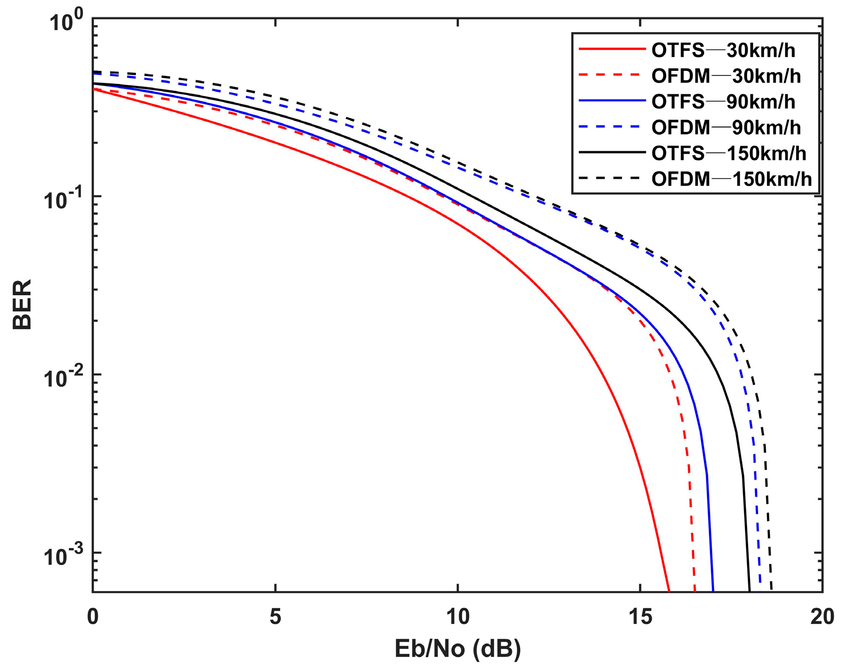
In Figure 4, the BER is compared for the two modulation modes at different speeds. It can be seen that BER becomes larger as the flight speed of the UAV increases, which indicates that the Doppler shift from high speed-movement can seriously affect the communication quality. We also note that the difference in BER between the two modulation modes becomes larger as the SNR increases. This means that the OTFS modulation mode requires a lower SNR than the OFDM modulation mode for the same communication conditions. In other words, the communication range of the UAV can be increased by using the OTFS modulation mode. Therefore, the OTFS modulation mode is expected to play an important role in high-mobility channel communication.

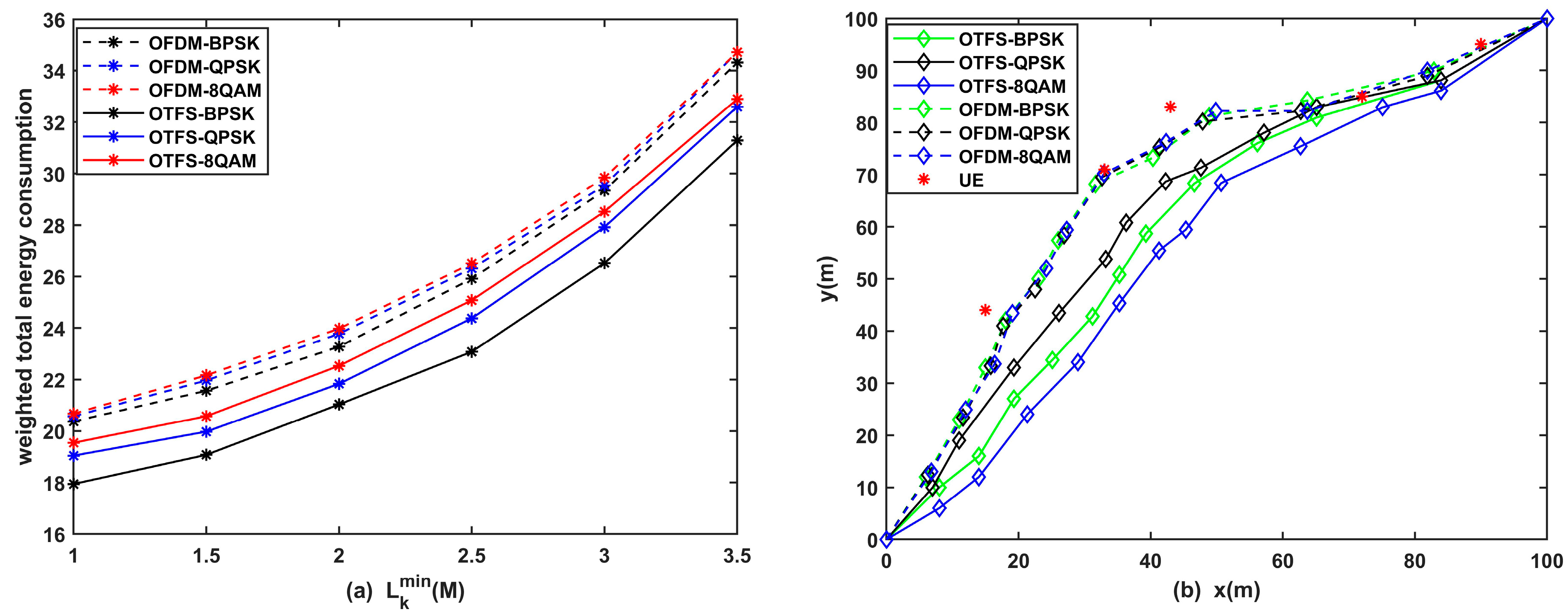
Figure 5 shows the weighted total energy consumption and flight trajectory for both OTFS and OFDM modes. From Figure 5a, the weighted total energy consumption of both schemes increases with the amount of minimum data. It can be seen that the OTFS system performs better than OFDM regardless of the modulation technique. In particular, the weighted total energy consumption of OTFS in BPSK modulation is significantly lower than that of OFDM. From Figure 5b, we can see that compared with the conventional OFDM mode, the UAV does not need to be too close to the UEs in OTFS mode. The reason for this phenomenon is that under high-speed movement, the UAV shows good robustness to the Doppler effect, and OTFS can obtain greater diversity gain in time and frequency. In other words, the UAV has a larger communication range when using the OTFS modulation technique under the same communication conditions. Therefore, the UAV will try to shorten the distance to achieve energy saving.

Figure 6 illustrates the sum energy consumption versus the different minimum data. The energy consumption of all schemes increases with the increase in the number of bits $L_k^{\min }$. The reason for the phenomenon is that when the amount of data is comparatively small, the UAV and UEs can effectively optimize resources. When the data are too large, the system needs to call on limited resources to complete the task as much as possible, resulting in a sharp increase in the weighted sum energy consumption. In other words, the more data, the smaller the resources that can be optimized. Notably, the sum energy consumption of the proposed algorithm is considerably less than that of the AOS, CXO and PSO algorithm, which indicates that the proposed algorithms are effective.

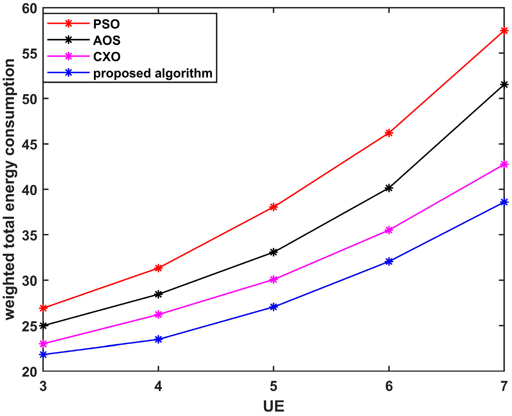
Figure 7 illustrates the weighted energy consumption of four schemes with a varying number of UEs. It can be seen that energy consumption increases with the number of UEs. However, the weighted energy consumption of the proposed algorithm is smaller than that of the other algorithms, indicating the effectiveness of the algorithm. It is worth noting that when the number of UEs is relatively small, the difference in the weighted total energy consumption of the four schemes is not large. However, as the number of UEs increases, the weighted total energy consumption of the proposed algorithm is much smaller than the other schemes, which suggests that the scheme can better adapt the multi-UEs scenarios.

In order to reveal the relationship of energy consumption between UEs and the UAV, the actual energy consumption of the two devices is plotted in various values of ${\mu }_1$ in Figure 8. This illustrates that as ${\mu }_1$ increases, the energy consumption of UEs decreases while that of UAV increases, which also verifies Theorem 1. The more valuable the UE energy, the larger the amount of energy required to be consumed by the UAV to meet the minimum computational requirements. Note that the actual energy consumption of the UAV does not increase monotonically with ${\mu }_1$. On the one hand, the UAV energy of the UAV is weighted so that the real energy of UAV fluctuates within a certain range without affecting the target value. On the other hand, constrained by flight resources of the UAV, the energy consumption tends to the upper limit. In conclusion, UEs and the UAV always cooperate in carrying out the task.

In Figure 9, the weighted energy consumption of the UE and the system at different time slots are plotted to reveal the impact of UAV position on UEs. Figure 9a shows that the different positions of the UAV have great influence on the energy consumption of the UE. When the UAV is close to the UE, the energy consumption of the UE is relatively low. It is worth noting that when the energy consumption of the system is the lowest, the energy consumption of all UEs is relatively low. The reason is that the first half of the UAV will be close to the favorable service position, and the second half will rapidly become far away from the favorable service position. When the UAV reaches a favorable service position, it will fly slowly to reduce energy consumption. In brief, Figure 9 shows that trajectory optimization can effectively reduce the sum energy consumption of the system.

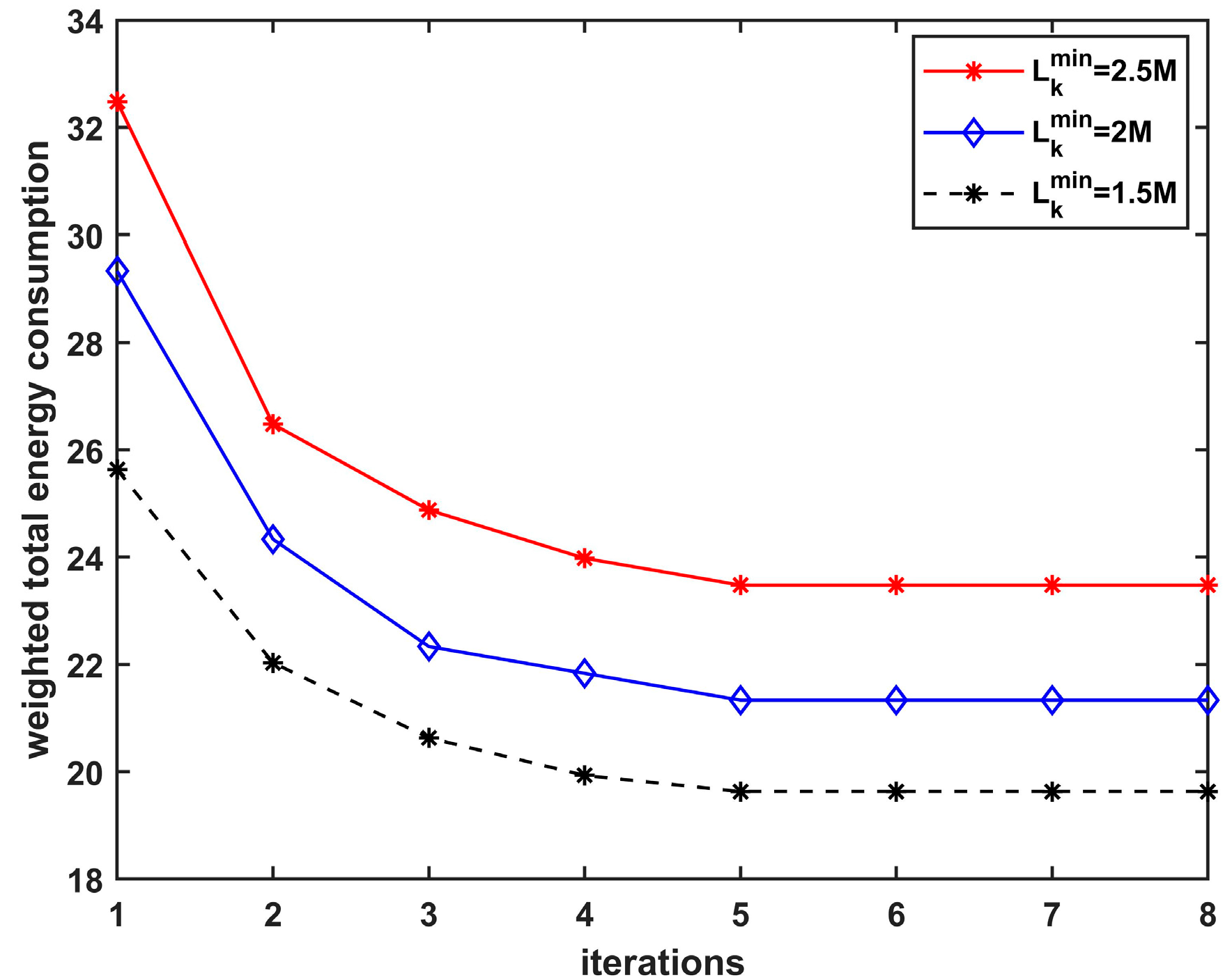
Figure 10 depicts the iterations of the weighted total energy under the three schemes. It can be seen that the weighted total energy consumption decreases more obviously in the first and second iterations, and the third basically tends toward stability. The reason for this phenomenon is that the proposed iterative algorithm is far from the optimal position in the first two iterations, and the UE needs to consume a lot of energy to complete the task. In the third iteration, all optimization variables remain almost stable, and a better solution is obtained. This further verifies the convergence of the algorithm.

Finally, in Figure 11, we analyze the weighted total energy consumption under different values of time slot division (t denotes the variable $t_{}^o[n]$). It can be seen that when the values are very low, the energy consumption of the four schemes is also low and similar. With the increase in $L_k^{\min }$, the energy of the benchmark algorithms will increase greatly after exceeding a certain threshold. However, the proposed algorithm can complete the task with lower energy consumption, which is more obvious. The reason for the phenomenon is that within a limited time and with an increase in data, UEs or the UAV can only offload a large number of tasks that cannot be processed by adjusting the transmit power, but there is a threshold upper limit for the transmission power. The proposed algorithm can automatically allocate the time slot size, raise the upper limit of the threshold, and effectively reduce transmit power to reduce energy consumption. This demonstrates that time slot optimization plays an important role in reducing total energy consumption.

5. Conclusions

In this paper, we propose resource allocation and trajectory optimization in OTFS based UAV-assisted MEC for severe Doppler effects caused by high-speed motion. The weighted total energy consumption of the system is minimized by jointly optimizing the time division, CPU frequency allocation, transmit power allocation and flight trajectory under the premise of considering Doppler compensation. A joint algorithm combining the advantages of the heuristic algorithm and convex optimization algorithm is proposed for the above nonconvex problem. The simulation results demonstrate that the OTFS-based UAV system outperforms the OFDM-based UAV system, and the proposed algorithm is superior to the convex optimization and heuristic algorithm. In future research, we will focus on multiple UAVs and multiple UEs, and move to real-world scenarios as soon as possible.

References

- Chiang, M.; Zhang, T. Fog and IoT: An overview of research opportunities. IEEE Internet Things J. 2016, 3, 854–864. [Google Scholar] [CrossRef]
- Mach, P.; Becvar, Z. Mobile edge computing: A survey on architecture and computation offloading. IEEE Commun. Surv. Tutor. 2017, 19, 1628–1656. [Google Scholar] [CrossRef]
- Apostolopoulos, P.A.; Fragkos, G.; Tsiropoulou, E.E.; Papavassiliou, S. Data offloading in UAV-assisted multi-access edge computing systems under resource uncertainty. IEEE Trans. Mob. Comput. 2021, 22, 175–190. [Google Scholar] [CrossRef]
- Kato, N.; Fadlullah, Z.M.; Tang, F.; Mao, B.; Tani, S.; Okamura, A.; Liu, J. Optimizing space-air-ground integrated networks by artificial intelligence. IEEE Wirel. Commun. 2019, 26, 140–147. [Google Scholar] [CrossRef]
- Zeng, Y.; Rui, Z.; Teng Joon, L. Wireless communications with unmanned aerial vehicles: Opportunities and challenges. IEEE Commun. Mag. 2016, 54, 36–42. [Google Scholar] [CrossRef]
- Guo, F.; Zhang, H.; Ji, H.; Li, X.; Leung, V.C.M. An efficient computation offloading management scheme in the densely deployed small cell networks with mobile edge computing. IEEE/ACM Trans. Netw. 2018, 26, 2651–2664. [Google Scholar] [CrossRef]
- Liu, Y.; Wu, F.; Lyu, C.; Li, S.; Ye, J.; Qu, X. Deep dispatching: A deep reinforcement learning approach for vehicle dispatching on online ride-hailing platform. Transp. Res. Part E Logist. Transp. Rev. 2022, 161, 102694. [Google Scholar] [CrossRef]
- Jiang, H.; Peng, D.; Yang, K.; Zeng, Y.; Chen, Q. Predicted mobile data offloading for mobile edge computing systems. In International Conference on Smart Computing and Communication; Springer: Berlin/Heidelberg, Germany, 2018; pp. 153–162. [Google Scholar]
- Chen, M.; Mozaffari, M.; Saad, W.; Yin, C.; Debbah, M.; Hong, C.S. Caching in the sky: Proactive deployment of cache-enabled unmanned aerial vehicles for optimized quality-of-experience. IEEE J. Sel. Areas Commun. 2017, 35, 1046–1061. [Google Scholar] [CrossRef]
- Huang, L.; Feng, X.; Feng, A.; Huang, Y.; Qian, L.P. Distributed deep learning-based offloading for mobile edge computing networks. Mob. Netw. Appl. 2018, 27, 1123–1130. [Google Scholar] [CrossRef]
- Jiang, F.; Wang, K.; Dong, L.; Pan, C.; Xu, W.; Yang, K. Deep-learning-based joint resource scheduling algorithms for hybrid MEC networks. IEEE Internet Things J. 2019, 7, 6252–6265. [Google Scholar] [CrossRef]
- Li, M.; Cheng, N.; Gao, J.; Wang, Y.; Zhao, L.; Shen, X. Energy-Efficient UAV-Assisted Mobile Edge Computing: Resource Allocation and Trajectory Optimization. IEEE Trans. Veh. Technol. 2020, 69, 3424–3438. [Google Scholar] [CrossRef]
- Zhang, T.; Xu, Y.; Loo, J.; Yang, D.; Xiao, L. Joint computation and communication design for UAV-assisted mobile edge computing in IoT. IEEE Trans. Ind. Inform. 2019, 16, 5505–5516. [Google Scholar] [CrossRef]
- Ji, J.; Zhu, K.; Yi, C.; Niyato, D. Energy consumption minimization in UAV-assisted mobile-edge computing systems: Joint resource allocation and trajectory design. IEEE Internet Things J. 2020, 8, 8570–8584. [Google Scholar] [CrossRef]
- Liu, B.; Wan, Y.; Zhou, F.; Wu, Q.; Hu, R.Q. Resource allocation and trajectory design for miso uav-assisted mec networks. IEEE Trans. Veh. Technol. 2022, 71, 4933–4948. [Google Scholar] [CrossRef]
- Xu, Y.; Zhang, T.; Liu, Y.; Yang, D.; Xiao, L.; Tao, M. UAV-assisted MEC networks with aerial and ground cooperation. IEEE Trans. Wirel. Commun. 2021, 20, 7712–7727. [Google Scholar] [CrossRef]
- Bai, L.; Han, R.; Liu, J.; Yu, Q.; Choi, J.; Zhang, W. Air-to-ground wireless links for high-speed UAVs. IEEE J. Sel. Areas Commun. 2020, 38, 2918–2930. [Google Scholar] [CrossRef]
- Hadani, R.; Rakib, S.; Tsatsanis, M.; Monk, A.; Goldsmith, A.J.; Molisch, A.F.; Calderbank, R. Orthogonal time frequency space modulation. In Proceedings of the IEEE Wireless Communications and Networking Conference (WCNC), San Francisco, CA, USA, 19–22 March 2017. [Google Scholar]
- Hadani, R.; Monk, A. OTFS—A novel modulation technique meeting 5G high mobility and massive MIMO challenges. White Pap. 2017. [Google Scholar]
- Kumar, A.; Perveen, S.; Singh, S.; Kumar, A.; Majhi, S.; Das, S.K. 6th Generation: Communication, Signal Processing, Advanced Infrastructure, Emerging Technologies and Challenges. In Proceedings of the 2021 6th International Conference on Computing, Communication and Security (ICCCS), Las Vegas, NV, USA, 4–6 October 2021. [Google Scholar]
- Singh, P.; Gupta, A.; Mishra, H.B.; Budhiraja, R. Low-complexity ZF/MMSE MIMO-OTFS receivers for high-speed vehicular communication. IEEE Open J. Commun. Soc. 2022, 3, 209–227. [Google Scholar] [CrossRef]
- Liang, Y.; Li, L.; Fan, P.; Guan, Y. Doppler resilient orthogonal time-frequency space (OTFS) systems based on index modulation. In Proceedings of the 2020 IEEE 91st Vehicular Technology Conference (VTC2020-Spring), Antwerp, Belgium, 25–28 May 2020. [Google Scholar]
- Bhat, V.S.; Chockalingam, A. Performance Analysis of OTFS Modulation with Transmit Antenna Selection. In Proceedings of the 2021 IEEE 93rd Vehicular Technology Conference (VTC2021-Spring), Helsinki, Finland, 25–28 April 2021. [Google Scholar]
- Jeong, S.; Simeone, O.; Kang, J. Mobile edge computing via a UAV-mounted cloudlet: Optimization of bit allocation and path planning. IEEE Trans. Veh. Technol. 2017, 67, 2049–2063. [Google Scholar] [CrossRef]
- Messous, M.A.; Senouci, S.M.; Sedjelmaci, H.; Cherkaoui, S. A game theory based efficient computation offloading in an UAV network. IEEE Trans. Veh. Technol. 2019, 68, 4964–4974. [Google Scholar] [CrossRef]
- Wu, Q.; Zeng, Y.; Zhang, R. Joint trajectory and communication design for multi-UAV enabled wireless networks. IEEE Trans. Wirel. Commun. 2018, 17, 2109–2121. [Google Scholar] [CrossRef]
- Wei, Z.; Yuan, W.; Li, S.; Yuan, J.; Bharatula, G.; Hadani, R.; Hanzo, L. Orthogonal time-frequency space modulation: A promising next-generation waveform. IEEE Wirel. Commun. 2021, 28, 136–144. [Google Scholar] [CrossRef]
- Reddy, C.S.; Sen, D.; Singhal, C. Performance analysis of NR based vehicular IoT system with OTFS modulation. In Proceedings of the 2021 IEEE 94th Vehicular Technology Conference (VTC2021-Fall), Norman, OK, USA, 27–30 September 2021. [Google Scholar]
- Bi, S.; Zhang, Y.J. Computation rate maximization for wireless powered mobile-edge computing with binary computation offloading. IEEE Trans. Wirel. Commun. 2018, 17, 4177–4190. [Google Scholar] [CrossRef]
- Wang, Y.; Sheng, M.; Wang, X.; Wang, L.; Li, J. Mobile-edge computing: Partial computation offloading using dynamic voltage scaling. IEEE Trans. Commun. 2016, 64, 4268–4282. [Google Scholar] [CrossRef]
- Zeng, Y.; Xu, J.; Zhang, R. Energy minimization for wireless communication with rotary-wing UAV. IEEE Trans. Wirel. Commun. 2019, 18, 2329–2345. [Google Scholar] [CrossRef]
- Azizi, M. Atomic orbital search: A novel metaheuristic algorithm. Appl. Math. Model. 2021, 93, 657–683. [Google Scholar] [CrossRef]
- Boyd, S.; Vandenberghe, L. Convex Optimization; World Publishing Corporation: Cleveland, NY, USA, 2004. [Google Scholar]
Figure 1.
The system model.
Figure 2.
OTFS modulation model.
Figure 3.
The time slot division.
Figure 4.
The BER of different speeds in two modulation modes.
Figure 5.
(a) The weighted total energy consumption under different modulation modes. (b) The flight path under different modulation modes.
Figure 6.
Weighted sum energy consumption versus data for four algorithms.
Figure 7.
The weighted sum energy consumption versus UEs quantity for four algorithms.
Figure 8.
Real energy consumption comparison of UEs and the UAV with varying weight .
Figure 9.
(a) The weighted energy consumption of UEs with varying time slot. (b) The weighted total energy consumption with varying time slot.
Figure 10.
The weighted sum energy consumption versus the number of iterations.
Figure 11.
The weighted total power consumption versus the different time slots.