
Power Transformer Fault Diagnosis Based on Improved BP Neural Network

1
School of Mechanical Engineering and Rail Transit, Changzhou University, Changzhou 213164, China
2
Jiangsu Yude Xingyan Intelligent Technology Co., Ltd., Changzhou 213164, China
3
Jiangsu Province Engineering Research Center of High-Level Energy and Power Equipment, Changzhou University, Changzhou 213164, China
4
School of Computer Science and Artificial Intelligence, Changzhou University, Changzhou 213164, China
*
Authors to whom correspondence should be addressed.
Electronics 2023, 12(16), 3526; https://doi.org/10.3390/electronics12163526
Submission received: 14 July 2023
/
Revised: 31 July 2023
/
Accepted: 31 July 2023
/
Published: 21 August 2023
(This article belongs to the Special Issue Machine Learning in Power System Monitoring and Control)
Abstract
:Power transformers are complex and extremely important piece of electrical equipment in a power system, playing an important role in changing voltage and transmitting electricity. Its operational status directly affects the stability and safety of power grids, and once a fault occurs, it may lead to significant economic losses and social impacts. The traditional detection methods rely on the technical level of power system operation and maintenance personnel, and are based on Dissolved Gas Analysis (DGA) technology, which analyzes the components of dissolved gases in transformer oil for preliminary fault diagnosis. However, with the increasing accuracy and intelligence requirements for transformer fault diagnosis in power grids, the DGA analysis method is no longer able to meet the requirements. Therefore, this article proposes an improved transformer fault diagnosis method based on a residual BP neural network. This method deepens the BP neural network by stacking multiple residual network modules, and fuses and expands gas feature information through an improved BP neural network. In the improved residual BP neural network, SVM is introduced to judge the extracted feature vectors at each layer, screen out feature vectors with high accuracy, and increase their weights. The feature vector with the highest cumulative weight is selected as an input for transformer fault diagnosis. This method utilizes multi-layer neural network mapping to extract gas feature information with more significant feature differences after fusion expansion, thereby effectively improving diagnostic accuracy. The experimental results show that, compared with traditional BP neural network methods, the proposed algorithm has higher accuracy in transformer fault diagnosis, with an accuracy rate of 92%, which can ensure the sustainable, normal, and safe operation of power grids.
1. Introduction
With the continuous development of our economy and the continuous improvement in the quality of people’s living standards, people’s daily life, industrial production and transportation all have a close relationship with power [1,2]. With the development of the economy, not only is the scale of our power grid expanding, the substation is increasing, power transmission occurs from west to east, a cross-regional power grid pattern is gradually formed, and the power system will meet more and more challenges [3,4]. In the whole power grid system, any failure or accident will have an impact on the operation of the whole power grid. When there is a large-scale power failure or system failure, it will cause huge losses to the national economy, and seriously endanger public security and social stability [5]. The power transformer is the core equipment of the substation [6]. In the process of power transmission, the power generated by the power plant is transmitted to the power grid through the step-up transformer, and each region and system are interconnected through the transformer. On the power side, the voltage is reduced to the required voltage level through the step-down transformer [7]. Therefore, the running state of the transformer directly affects the reliable operation of the power grid system, and plays a vital role in the normal power supply of people’s daily life [8,9].
Due to the defects of the transformer operating environment, transportation and installation [10,11], there are inevitably some local defects in the transformer, such as bubbles, cracks, electrode burrs, long-term deterioration, aging insulation and other problems; therefore, failures occur from time to time [12]. IEC 60599:2007 The “Interpretation guidelines for dissolved gas analysis of electrical equipment in operation with mineral insulating oils” reduced the original nine typical faults to six, namely, partial discharge, low-energy discharge, high-energy discharge, low-temperature overheating, medium-temperature overheating, and high-temperature overheating. Medium-temperature and low-temperature overheating can be combined into a single category, called medium-to-low-temperature overheating, resulting in a total of five fault types. When analyzing the types of transformer faults in domestic scenarios [13], overheating faults have the highest probability of occurrence, followed by high-energy discharge faults, low-energy discharge faults, and partial discharge faults, with the lowest occurrence rate being related to faults caused by transformer dampness or partial discharge.
The transformer plays an important role in the power grid system. If failure or accidents occur during operation, they will affect the power quality, damage related equipment, and cause personal injury and other malignant accidents. For example, in 2005, the winding insulation of Laiwu Station (110 kV) of Shandong Power Grid was seriously damaged due to the inter-turn short-circuit discharge fault. With the continuous development of science and technology, the circuit department attaches more and more importance to transformer failures and hidden dangers [14], and adopts such methods, such as inspection and elimination, to reduce the probability of transformer failures, but it is still difficult to avoid transformer failures. Therefore, it is urgent to study the transformer fault diagnosis and operation monitoring, so that the power department can find the existing faults and hidden dangers as early as possible, according to the actual problems, deal with problems in the bud stage, and extend its service life. With the continuous progress of science and technology, the capacity of a single transformer is increasing, its internal structure is becoming more and more complex, and the mutual influence and interaction between different internal components are becoming closer, which increases the difficulty of transformer fault diagnosis to some extent [15,16]. By improving the accuracy of transformer fault diagnosis methods, it is possible to promptly detect and repair faults, ensuring the reliability and stability of the electricity supply.
Currently, the development of Dissolved Gases Analysis (DGA) technology in oil has become relatively mature [17]. Based on DGA technology, some traditional diagnostic methods, such as the IEC three-ratio method, modified three-ratio method, and Rogers ratio method, have been applied in practical transformer fault diagnosis. However, these traditional diagnostic methods inevitably have certain flaws, such as limited usage conditions and incomplete ratio encoding [18,19]. With the development of intelligent algorithms, most researchers have started combining DGA diagnostic results with intelligent diagnostic methods to improve the accuracy of transformer fault prediction. Common intelligent diagnostic methods include the BP neural network [20] and the Support Vector Machine (SVM) model [21], etc.
The literature [22] proposes a method that combines neural networks and the three-ratio method to convert samples with diagnostic errors from neural networks to the three-ratio method for diagnosis. However, the accuracy of neural network judgments depends on the selection of weights and thresholds, and requires a large amount of training data, making the operation complex and the stability insufficient. Moreover, the optimal threshold is prone to change with different quantities of sample data. Xu Xin et al. utilized locust swarm optimization to optimize certain parameters of the BP neural network, improving its speed and search abilities, but its network performance was poor and the learning rate was unstable [23]. In the literature [24], a transformer fault intelligent diagnosis method combining empirical wavelet transform and improved convolutional neural network is proposed. The results show that this diagnostic model can effectively identify the fault states of transformers. When using the SVM model for fault diagnosis, the kernel function and penalty factor in the model limit its classification performance. Improper values can lead to significant prediction errors. Therefore, various bio-inspired optimization algorithms [25] are introduced to enhance the predictive ability of the SVM model for transformer faults. In practical applications, the aforementioned methods can solve the cumbersome steps and absolute diagnosis issues of traditional methods, but the further optimization of training accuracy and improvements in adaptability are needed.
In addition, during the daily operation of the transformer, the failure is an accidental event, and the probability is small, so it is difficult to obtain a large amount of fault data [26]. The lack of samples and the diversity of faults further increase the difficulties in transformer fault diagnosis and make it difficult to diagnose and predict transformer faults only by human experience. Accurate transformer fault diagnosis methods can assist maintenance personnel in quickly identifying the type and location of faults, thereby improving the efficiency of troubleshooting. This is crucial for power grids because rural areas typically have limited human and material resources, and the efficiency of fault-handling directly affects the normal operation of the grid. When fault diagnosis is carried out using artificial intelligence, sufficient historical data should be supported. Only with large and comprehensive data can the accuracy and practicability of the whole diagnosis system be guaranteed. This method has the problems of low accuracy and low diagnosis accuracy with limited information [27,28,29]. Although the diagnostic methods mentioned above have achieved certain results in the diagnosis of transformer faults, the overall diagnostic accuracy is still insufficient. At the same time, the above diagnosis method, based on a traditional BP neural network, still has problems of low diagnostic accuracy in shallow models and poor diagnostic accuracy when there are few sample data. This method is based on the residual backpropagation (BP) neural network, and its purpose is to improve the accuracy and reliability of transformer fault diagnosis, ensuring the stability and safe operation of the power grid. In this method, each residual network module in this paper consists of two layers of BP neural networks. Residual learning is utilized to transform the identity mapping learning in the conventional BP neural network. In addition, the input information of each remaining network module can be transmitted on one layer of the network to better extract feature information from transformer fault data. In the improved residual BP neural network, a support vector machine (SVM) is introduced to evaluate the feature vector extracted by each layer; the vector with high diagnostic accuracy is selected and its weight is increased. Finally, the eigenvector with the highest cumulative weight is selected for transformer fault diagnosis. Therefore, the improved residual BP neural network model exhibits an excellent diagnostic performance even with few sample data.
In conclusion, the improved residual backpropagation (BP) neural network transformer fault diagnosis method proposed in this paper effectively addresses the cumbersome steps and absolutization issues present in traditional methods, while maintaining high training accuracy and adaptability. The fault diagnosis based on the residual BP neural network makes the diagnosis of transformer faults easier, significantly reducing maintenance frequency, minimizing repair costs, shortening planned outage time for transformers, saving resources in terms of manpower and materials, alleviating maintenance burden, and enhancing the operational reliability of transformers [30].
Relevant data indicate that implementing fault diagnosis measures under transformer operating conditions can lead to a reduction in annual maintenance costs of 25–50% and a decrease in fault-related downtime of 75% [31,32]. A survey conducted in the UK on 2000 state-owned projects showed that adopting fault diagnosis technology could save up to 300 million pounds in annual maintenance costs [33]. Therefore, adopting the residual BP neural-network-based fault diagnosis method for power transformers can effectively promote the implementation of condition-based maintenance and yield significant economic benefits [34].
2. Transformer Fault Analysis and Detection
2.1. Common Faults of Transformers
2.1.1. Electrical Fault
The phenomenon of the rapid deterioration of the insulation part of the transformer caused by electrical stress is called “electrical failure”, which has a high level of energy density. According to the electrical fault in the deterioration process, and the energy and energy density of the fault location, the electrical fault can be further refined into three types, namely partial discharge, low-energy discharge, and high-energy discharge. Partial discharge is the initial stage of the electrical failure of a transformer. If bubbles are present in the insulating oil in the transformer, it may be that the manufacturing means are incomplete or the industrial operation is not standardized, resulting in inferior structures such as voids, impurities, and moisture in the insulation material. Temperature changes may also cause the paint surface to be unsmooth; when metal parts are not in close enough contact, this can cause them to loosen and fall off, and partial discharge may occur. The energy density at the first and last ends of the conductor is not large, but if it is not included in time, it leads to internal discharge. Low-energy discharge, also known as “spark discharge”, can occur due to the different manufacturing structures of the transformer, or poor contact during distribution, assembly and operation, loosening, etc. If elements in the voltage position (fastening bolts, transverse magnetic barriers, etc.) appear, they are isolated (loose, etc.). This occurs in the grounding part, causing a high-potential floating discharge between the grounding potential components, resulting in a low-energy discharge. When high-energy discharge, also known as “arc discharge”, occurs, the energy density will be quite large, resulting in a severely insulating oil cracking reaction, producing a fault characteristic gas. Discharge will cause the insulation between the windings to break down, for example, through carbonization and the destruction of insulating paper, and even the thermal deformation and aging of metal parts. It can also cause flashover, breakage and tap-changer of transformer leads, arc flicker, etc. Table 1 shows the specific faults corresponding to the transformer fault types.
2.1.2. Thermal Failure
Thermal failure occurs when the insulating oil in a transformer rapidly deteriorates due to thermal stress, resulting in a relatively low energy density during degradation.
According to fault data statistics, approximately 50% of all thermal faults can be attributed to the characteristics of thermal stress in transformer faults and the closed positions of components like tap-changers. About 20% of thermal faults are caused by short-circuits, magnetized inrush currents, and leakage flux loops. Additionally, faults arising from core overheating due to short-circuits and discharges caused by multi-point grounding account for around 30% of all thermal faults.
2.2. Dissolved Gas Analysis in Oil
2.2.1. Principle of Dissolved Gas Generation in Power Transformers
When the power transformer is abnormal, a variety of hydrocarbon gases will be produced inside the transformer. These gases have different properties in different concentrations. We collected the concentrations of these gases and used other data to judge the transformer failure. These oil-dissolved gases mainly fall into the following three categories.
- (a)
- Decomposition of insulating oil
Transformer oil is a product extracted from petroleum; its main components are alkanes, naphthenic saturated hydrocarbons, aromatic unsaturated hydrocarbons and other compounds, commonly known as square shed oil. After the failure of the power transformer, some C-H bonds, C-C bonds and O-H bonds will be broken, and after the chemical bonds are broken, hydrogen atoms and a large number of hydrocarbons will produce free radicals. These hydrogen atoms and free radicals undergo various chemical reactions to form hydrocarbon gases and hydrogen . Chemical bonds require different energies when breaking; C-H and O-H chemical bond fractures require less energy, so most of the energy generated by the fault is enough to break its chemical bond to form a new substance. , and C≡ C, C≡C chemical bond-breaking requires higher bond energies. In the event of medium- and low-temperature overheating, low-energy discharge and high-energy discharge failure will produce enough bond energy to break it, forming a new gas (, , , etc.).
- (b)
- Decomposition of solid insulating materials
There are many types of solid insulation materials for transformers, such as insulating paper, electrical laminated wood, epoxy glass cloth, low-dielectric-loss laminate, insulating paint, insulating glue, cotton cloth tape, and mesh weft free polyester tape. These materials are composed of more C-H keys. After transformer failure, these insulation materials will decompose, producing a large amount of , gas, and a small amount of water and hydrocarbon gas.
- (c)
- Other sources
The gas produced by the transformer is not necessarily caused by transformer failure; there are also some objective reasons for the production of gas, such as the environment, weather and manufacturing process. When the temperature is high, the trace oxygen () dissolved in the oil reacts with the paint of the internal device of the transformer to produce a certain amount of . Trace amounts of water () dissolved in the oil react with the ferrous components inside the transformer to produce a small amount of . During the later maintenance and repair of the transformer, gases such as carbon dioxide () in the air will also be absorbed by the transformer’s insulating oil, and the oil will also produce certain gases under sunlight.
2.2.2. Gas Generation in Transformer Oil
Power transformer under the action of heat, electricity, magnetism and insulating oil will produce impurities to deteriorate the transformer insulating oil, or a certain amount of gas will appear in the insulating oil, according to the type of gas, concentration, gas production rate, etc. This can be used to judge whether the transformer has failed.
- (a)
- Judge according to gas concentration
When the transformer is working, hydrocarbon gases will be produced. If the transformer works normally and under fault conditions, the gas composition and content in the insulation oil will be very different. We can judge whether the transformer has failed by detecting the gas content. The limit value of each gas content under the normal working state of the transformer is shown in Table 2:
- (a)
- Judge according to the gas production rate
When the transformer fails, in many cases, the dissolved gas content in the insulating oil is very low, sometimes resulting in the transformer fault diagnosis not eing timely enough. If this situation is maintained for a long time, the transformer may undergo more serious failure, leading to damage, shutdown and even explosion. Whether the transformer has failed can be determined according to the gas production rate in the transformer oil. Specifically, this can be divided into absolute gas production rate and relative gas production rate, and the formula is as follows:
—absolute gas production rate (mL/d).
—relative gas production rate (mL/d).
—gas concentration in oil at first measurement (L/L).
—gas concentration in oil (L/L) on the second measurement.
—time difference between two measurements (d).
m—transformer insulating oil (t).
P—transformer insulating oil density (t/).
The critical values for the absolute gas production rate of transformer oil are shown in Table 3.
2.2.3. Dissolved Gas Composition in Oil
After the transformer fails, the dissolved gas in the transformer oil reaches more than a dozen, these gas components and content are of great significance to the transformer fault diagnosis, domestic transformer fault diagnosis, commonly used gases are , , , , , , these seven gases, of which , combination is often used to diagnose whether the transformer solid insulation material fails, , combination is often used to diagnose whether the transformer occurs partial discharge fault, , The combination of is used to diagnose whether the transformer has a thermal fault, and the different faults and their corresponding gas components are shown in Table 4.
2.2.4. Dissolution of Gases
The bubble generation comes from cracking, which is generated by the cracking of the insulating material in the vessel, and the bubbles will disperse after they are generated and slowly melt into the oil. Differences in oil temperature in the transformer can lead to oil circulation. When the cyclic movement begins, the gas will slowly move to the rest of the transformer. When a fault arises, a large amount of fault gas is generated. The Osterwald coefficient Ki is often used to calculate the solubility of a gas. As long as the concentration of the gas components in the gas is measured, the Osterwald coefficient, derived from the equilibrium principle, can be used to calculate the gas dissolution. The concentration in transformer oil is derived using the Osterwald formula, as shown in (3):
—component concentration refers to the gas dissolved in oil;
—refers to the concentration of the gas component I; the Oerswald coefficient is .
The Oerswald coefficients for various gases in transformer oil are shown in Table 5.
When a potential failure occurs in the transformer, gas and bubbles will be generated when gas is generated at a high speed, and some of the gases and bubbles in the transformer oil will melt into the oil. The smaller the bubble, the greater the viscosity of the oil and the slower the bubble floats, meaning that the bubble is in total contact with the transformer oil, so that the gas replacement is more complete. Of course, some losses occur when the gas is dissolved in the transformer oil by diffusion and convection. For example, due to temperature differences, gas will be transferred from inside the fuel tank of the transformer to the oil level and storage tank. When the transformer is operating, the gases adsorbed by these solids are redissolved in the transformer oil.
2.3. Transformer Fault Diagnosis Method
The fault diagnosis methods of transformers are summarized into two categories, namely, the traditional transformer fault diagnosis method and the intelligent transformer fault diagnosis method, as shown in Figure 1.
2.3.1. Traditional Transformer Fault Diagnosis Method
- (a)
- Characteristic gas method
According to Table 4, the gas composition of different fault types can be known, which can be used to determine the category of transformer fault. This method is called the characteristic gas method. The relationship between transformer fault categories and characteristic gases is shown in Table 6.
- (b)
- Ratio method
- 1.
- IEC triple-ratio method
IEC three-ratio method was originally proposed by the International Electrotechnical Commission (IEC) in the study of thermodynamic theory. The IEC three-ratio method is based on the relationship between the fault gas composition and temperature generated when transformer oil fails. Using the free combination of 0, 1, 2 to express the relationship between the three pairs of gas ratios, the three pairs of gas ratios are: /, /, /. This gas composition and coding combination is used to judge the transformer fault type, as shown in Table 7.
As shown in the above table, when the ratio of the three gases is less than 0.1, the ratio codes of the three gases are 0, 1, and 0, respectively. When the ratio of the three gases is greater than or equal to 0.1 and less than 1, their ratio codes are 1, 0 and 0, respectively. When the ratio of the three gases is greater than or equal to 1 and less than 3, their ratio codes are 1, 2 and 1, respectively. When the ratio of the three gases is greater than or equal to 3, their ratio codes are 2, 2, and 2, respectively. When using the three-ratio method for transformer fault diagnosis, it is necessary to obtain the three gas ratio codes according to Table 7, and then compare the coding combination with the fault type.
- 2.
- No coding ratio method
IEC three-ratio method, as a transformer fault diagnosis method, has the characteristics of being simple and convenient, but the fault code is sometimes missing, and the coding information corresponding to the fault state cannot be found. In order to solve the shortcomings of IEC three-ratio method fault diagnosis, many experts and scholars at home and abroad have proposed the “coding ratio method” by simulating a large number of actual cases of transformer failure. The troubleshooting of the uncoded ratio method is shown in Table 8.
2.3.2. Intelligent Diagnosis Method
In order to quickly and accurately diagnose transformer faults, it is difficult to rely only on traditional diagnosis methods, because the transformer structure and oil gas production mechanism are complex, so artificial intelligence algorithms are required for transformer fault diagnosis. There are many intelligent diagnosis methods for transformer faults, such as fuzzy theory algorithms, expert systems, support vector machines, and BP neural networks. The specific characteristics of the four algorithms are shown in Table 9, in these four algorithms, the BP neural network algorithm has a clear input–output relationship problem, and transformer fault diagnosis belongs to the multi-classification input and output problem. While the support vector machine is only suitable for binary classification problems, the BP neural network can have multiple inputs and outputs, providing it with a clear advantage in transformer fault diagnosis of the multi-classification problem compared to other intelligent algorithms. The network is also simpler and convenient, but has the disadvantage of very easily falling into the local minimum point and a slow convergence speed. Therefore, in this paper, while selecting the BP neural network algorithm, we should also optimize the BP algorithm based on the support vector machine classification. An analysis and comparison of traditional and intelligent diagnostic methods is shown in Table 9.
3. Model Construction Based on Improved BP Neural Network
The improved BP neural network model is based on the traditional BPNN. The model introduces the idea of a ResNet residual network module, and embeds SVM classifiers in the IV.and V.residual modules, which screens feature vectors that have more influence on the accuracy of diagnostic results from the perspective of weights.
3.1. SVM Classifier
Support Vector Machine (SVM) algorithm is a classic binary classification algorithm, the core idea of which is to find an optimal hyperplane as the decision boundary, so as to maximize the distance between the decision-making boundary and the nearest two types of sample points, and the model based on this idea has been proved to have a good generalization ability. In the SVM algorithm, the sample point closest to the decision boundary is called the support vector, and the distance of the support vector from the decision hyperplane is defined as d, such that margin = 2 × d, as shown in Figure 2. The core of SVM is the optimization problem of finding the largest margin, i.e., d, under the qualification condition of effectively distinguishing between two types of samples.
According to the definition of the feature matrix, feature vector and sample label, it is assumed that the sample points are linear and divisible. Using the distance calculation formula in n-dimensional space, the distance from the sample point x as a support vector in Figure 2 to the decision hyperplane is:
of which is the modulus of the weight w, and b is the hyperplane intercept. Let the sample point label y = 1 be above the decision boundary in Figure 2 and the sample point label y = −1 be below, because the distance of all sample points xi from the decision boundary should be greater than d, according to Equation (4):
Divide the left and right ends of the inequality in Equation (5) by d at the same time; since ‖w‖ and d are constants, we can make , then Equation (5) can be equivalent to transform to:
As can be seen from Equation (6), Figure 2 ,. Make the same scaling of both ends of the hyperplane expression as shown in Equation (6): . Therefore, we can see that, for the support vector x, maximizing d is equivalent to maximizing , Whether the support vector is in the or hyperplane, there is , so the optimal index of SVM is to minimize the , that is, min. Simplifying Equation (6) yields ; in summary, the core idea of the SVM algorithm is the following conditional optimization problem:
For the above optimization objective function, the primary task of SVM is to ensure that the decision hyperplane can completely separate the two types of feature samples, but the generalization ability of the model under this goal will be limited and the common problem of linear indivisibility of data samples cannot be solved; therefore, the optimization objective function of SVM should be transformed into the following form:
Its aim is to introduce a loose operator to shift the hyperplane down ( up), thereby increasing the fault tolerance of the model to the training data set and improving the generalization ability of the model. The loose operator corresponds to m eigenvectors in eigenmatrix X, which are calculated as follows:
At the same time, to limit the fault tolerance of the model, should be introduced into the optimization objective function As the regularization term, C in Equation (8) is used as the weight hyperparameter, and the value of C can be dynamically adjusted by adjusting the value of C through the intelligent optimization algorithm to find the proportion of and in the optimization process.
The implementation logic of the linear classifier of SVM is given above; however, for transformer fault classification, because the distribution of data samples in the feature space is more complex, the use of linear classifier cannot obtain the best classification effect, so it is necessary to use the ascending method to map the originally linearly indivisible data into a higher-dimensional feature space to achieve linear separability. To do this, the concept of kernel function needs to be introduced.
In Equation (8), by solving the Lagrangian dual problem, the objective function of the optimization problem can be transformed into the following form:
For the paragraph in Equation (10), define polynomial kernel functions:
For n-dimensional eigenvectors, let , and expand Equation (11), which is equivalent to upgrading the eigenvectors and to , and then multiply them, so the quadratic polynomial kernel function can map the feature space of to the dimension, which greatly increases the data and the probability that a point is linear and divisible. In SVM, commonly used kernel functions are linear kernel functions: (equivalent to constructing linear SVMs), polynomial kernel functions: , and Gaussian kernel functions: , when using Gaussian kernel functions, and C as hyperparameters of the model, an intelligent optimization algorithm selection can be used.
3.2. Residual Network Module
When the neural network model reaches a certain depth, the diagnostic performance of the model will tend to be saturated and cannot be further improved; even the diagnostic performance will decrease with an increase in the number of network layers. The residual network (Figure 3) can convert the identity mapping of traditional neural networks into residual learning, which can solve the problems of gradient disappearance and gradient explosion caused by the increase in the number of network layers.
The first-layer residual network first weights its input data x, and calculates the ReLu activation function of its input data x to obtain the output , and the output of the second-layer residual network is as follows:
Formula: —Layer 2 network weights; —Layer 2 network biasing.
By adding the input data of the residual network of the previous layer, the residual network enables the current layer to obtain the original features of the data that have not been processed by the previous layer network and realizes residual learning, to ensure that the model can better extract feature information.
3.3. Improved Model Structure of BP Neural Network
The structure of the improved BP neural network model is shown in Figure 4.
Training set , .
The feature attribute dimension of the training set sample is h, the output vector dimension is f, and i represents the training sample group ordinal number in the training set.
Let represent the connection weight from the kth neuron of layer (L-1) to the jth neuron of layer represents the bias of the jth neuron at layer represents the jth nerve in layer l the activation value of the meta; is the ReLu activation function. The training set is divided into F categories, and the specific operation steps are as follows:
- (a)
- The output of the jth neuron of the l layer of the hidden layer is
Formula: S—number of neurons in layer (l-1) of the hidden layer; —feature vectors output by layer l in the hidden layer.
Taking the residual network modules V and VI as an example, when two hidden layers occur in the same residual network module, the output eigenvector is . When the two hidden layers are in different network modules, the output eigenvector is calculated by Equation (12), that is, the output of the module plus the input of the module.
The backpropagation of the error is shown in Equation (14), which updates and b according to the stochastic gradient descent method.
Formula: —weight increment; —bias increment; —learning rate, ; —the error is biased to the weight ; —the error derives the bias b.
- (b)
- Extract the feature vectors , of module V and module VI. and their corresponding category labels in the improved BP neural network to form a new training set , .
- (c)
- Use the new training set formed in step (b) to train the models TSVM1 and TSVM2 respectively, and the trained models are SVM1 and SVM2.
- (d)
- Input the validation set data into the network to extract the feature vectors and of the V. residual module and . residuals respectively, and then use SVM1 and SVM2 to diagnose the feature vectors and , respectively, and output the corresponding accuracy and .
- (e)
- If , calculate the weights of the eigenvectors according to Equation (15).
Formula: ,—indicates accuracy. The feature vector weights are and . corresponds to the average; corresponds to variance.
- (f)
- Update the feature vectors and of modules V and in step (b) to and , according to the new weights and obtained in step (e).
- (g)
- According to the expected output of the i-group sample of the output layer, the calculation error is ; see Equation (16).
4. Transformer Fault Diagnosis Based on Improved BP Neural Network
4.1. Fault Feature Selection
When the transformer is operating normally, the content of , , , , , is very small. When the low temperature is overheated, accounts for more than 27% of the total gas content, and when the medium temperature is overheated, the content decreases. When overheating at a high temperature, the content of is the highest, there is no in general partial discharge, and is increased. Generally, when discharging with low energy, the characteristic gas content is not much; mainly and . Therefore, the content of , , , , and in DGA is used as the fault diagnosis standard, and the overall operating state of the transformer is divided into six types: normal (), low-energy discharge (), high-energy discharge (), medium- and low-temperature overheating (), high-temperature overheating (), and partial discharge ().
4.2. Data Normalization
In order to reduce the difference between different characteristic gas content, the characteristic gas content value and the characteristic gas content ratio are normalized:
Formula: is the original amount of the gas content value or gas content ratio, . , are the maximum and minimum values of gas content or content ratio in the training set, respectively; is the normalized value after reasoning. Note that test set data also need to be normalized
4.3. Fault Type Code
This article divides power transformers into six categories according to the fault types in the operation process, and the fault type codes are shown in Table 10.
4.4. Filter Training Samples
The ultimate classification ability of a neural network is related to many factors; however, with other factors being equal, reliable training data can improve the classifier’s judgment ability. In order to further reduce the difference between different gas content values, the training data were selected using two metrics, Euler distance and Pearson coefficient, respectively.
- (a)
- Euler distance is a commonly used metric to calculate the natural length between vectors and is calculated as follows:
Formula: represents the Euclidean distance between the k-dimensional vector and ; and represent data points; m is the dimension of the vector;
- (b)
- The Pearson coefficient is a morphologically similar quantity, which solves the problem that the covariance is affected by dimensions. Its value range is [0,2], and the calculation formula is as follows:
Formula: Represents the Pearson coefficients of the k-dimensional vectors and .
According to Equations (18) and (19), the Euler distance and Pearson coefficient of the training data are calculated, respectively, and the data with the minimum value of both types of indicators are taken as the training data for this class.
4.5. Data Sampling Block
When training neural networks in distribution, different training sets need to be assigned to each subclassifier. In this paper, the Hermita polynomial interpolation method is used to interpolate and expand the original data. The red color in Figure 5 represents the data points obtained after applying 3 degrees of Hermita polynomial interpolation to the original data. Hermita polynomial interpolation is a method used to estimate values between given data points, effectively filling in the gaps and expanding the dataset. In this case, the original data points were interpolated to create additional data points, represented by the red color, to increase the size of the training set for each subclassifier in the distribution of neural networks.
Using the random sampling method, the interpolated and expanded training sample is divided into three training subsamples, and all the validation sets need to be put into each subsample, and >, according to < label, data, and type The data format is stored in HDFS (Distributed File System). “train” indicates training data, and its line begins with a label of 0 or 1; “val” indicates validation data, whose line prefix label is empty.
Interpolating and sampling the training data, on the one hand, can increase the size of training samples, provide more feature information yo the neural network, and make the training data meet the data requirements of distributed learning. On the other hand, random sampling can alleviate the imbalance in training data to a certain extent and solve the problem of bias in the training results.
4.6. Distributed Training
Read the training set and validation set required for model training from HDFS, and the number of subclassifiers is determined by the number of mappers in Spark. According to Equation (13), forward propagation is carried out and the model output is calculated. Update layers w and b according to Equation (14); When the error value shown in Equation (16) meets the requirements, the training ends.
Through the distributed training shown in Figure 6, each subclassifier can be obtained. Since each subtraining set is obtained by sampling, the data in each subtraining set are quite different, resulting in different parameters in each subclassifier. This means that the diagnostic performance of the final subclassifier is different.
4.7. Model Diagnosis
This paper introduces the idea of Adaboost, which votes on the classification results of Ci for the same new data, and takes the results of the subclassifier with the most votes as the final classification results. The model diagnosis process is shown in Figure 7.
5. Experimental Testing and Analysis
5.1. Data Sample Selection and Preprocessing
The residual BP neural network used in this paper has a total of seven residual network modules. At the time of training, the learning rate is 0.0001, the activation function is ReLU, there are a total of 250 rounds of training, the initial weight follows a Gaussian distribution with a mean of 0 and a standard deviation of 0.1, and the initial value of bias b is 0.01. A total of 415 transformer datasets [35] were used in this paper, of which 56, 67, 121, 47, 104, 20 are normal, low-energy discharge, high-energy discharge, medium–low-temperature overheating, high-temperature overheating, and partial discharge states, respectively. The data set was set up in the ratios of 6:4, 7:3 and 8:2 to establish the corresponding training set – and the test set –. In addition, in order to verify the effectiveness of the transformer fault diagnosis method proposed in this paper with few sample data, 112 pieces of data in the transformer dataset are taken as the training set S in the middle proportion of each fault category, and 56 (), 112 (), and 168 () pieces of data are taken as the test set in the remaining datasets.
5.2. Analysis of Transformer Fault Diagnosis Results
To evaluate the accuracy and reliability of the proposed transformer fault diagnosis method, we employed the confusion matrix as a crucial tool for results’ analysis, as shown in Figure 8. The confusion matrix provides an intuitive graphical representation, showcasing the classification performance of our proposed method across different fault categories and demonstrating a good diagnostic effectiveness for all six types of transformer fault. Through the confusion matrix, we can clearly observe a relationship between actual and predicted categories, enabling the further computation of various evaluation metrics to comprehensively assess the method’s performance.
To thoroughly investigate and evaluate the impact of different components on the proposed transformer fault diagnosis method, we conducted a series of ablation experiments. In these experiments, we enhanced the BP neural network model by introducing residual modules and integrating them with support vector machines (SVM). Through the ablation experiments, we compared and analyzed the effects of these variations on the diagnostic performance and presented the experimental results in tabular form. Table 11 displays the experimental outcomes for different model configurations, aiding in a better understanding and interpretion of the contributions of these components to transformer fault diagnosis. These experiments allow for us to comprehensively assess and validate the effectiveness and robustness of the proposed method.
Table 12 shows the diagnostic results of transformer fault data on the corresponding training and test sets of the improved residual BP neural network model, the traditional deep BP neural network model and the traditional shallow BP neural network model in this paper. As can be seen from Table 11, the improved residual BP neural network model maintains a high fault diagnosis accuracy under different test sets, with an average accuracy of 92.51%, and the diagnostic effect on each test set is relatively stable, with all remaining at 91.52% and above. The diagnostic accuracy of the traditional shallow BP neural network model is higher than that of the traditional deep BP neural network model, and the results show that the diagnostic performance of the traditional BP neural network decreases to a certain extent after an increase the network depth. In addition, the results shown in Table 11 show that the transformer fault diagnosis accuracy based on the improved residual BP neural network model is higher than that of the traditional shallow BP neural network and the traditional deep BP neural network model under different test sets, and the diagnostic results show that, after stacking multiple residual network modules, the number of layers of the deepening BP neural network not only does not decrease diagnostic performance compared with the traditional BP neural network, but leads to a significant improvement. Compared with the traditional shallow BP neural network and the traditional deep BP neural network, the diagnostic accuracy of the improved residual BP neural network model is improved by an average of 2.57% and 5.66%, respectively.
Table 13 shows the transformer fault diagnosis results based on an improved residual BP neural network model, traditional deep BP neural network model and traditional shallow BP neural network model with few sample data. It can be seen from Table 13 that, when there are few sample data, although the diagnostic accuracy of the improved residual BP neural network model decreases slightly with the increase in the number of test sample sets, the overall average diagnostic accuracy remains at 90.38%, which is 5.76% and 7.15% higher than that of the traditional shallow and deep BP neural network models. Furthermore, it is shown that the improved residual BP neural network model still has a good diagnostic performance with few sample data.
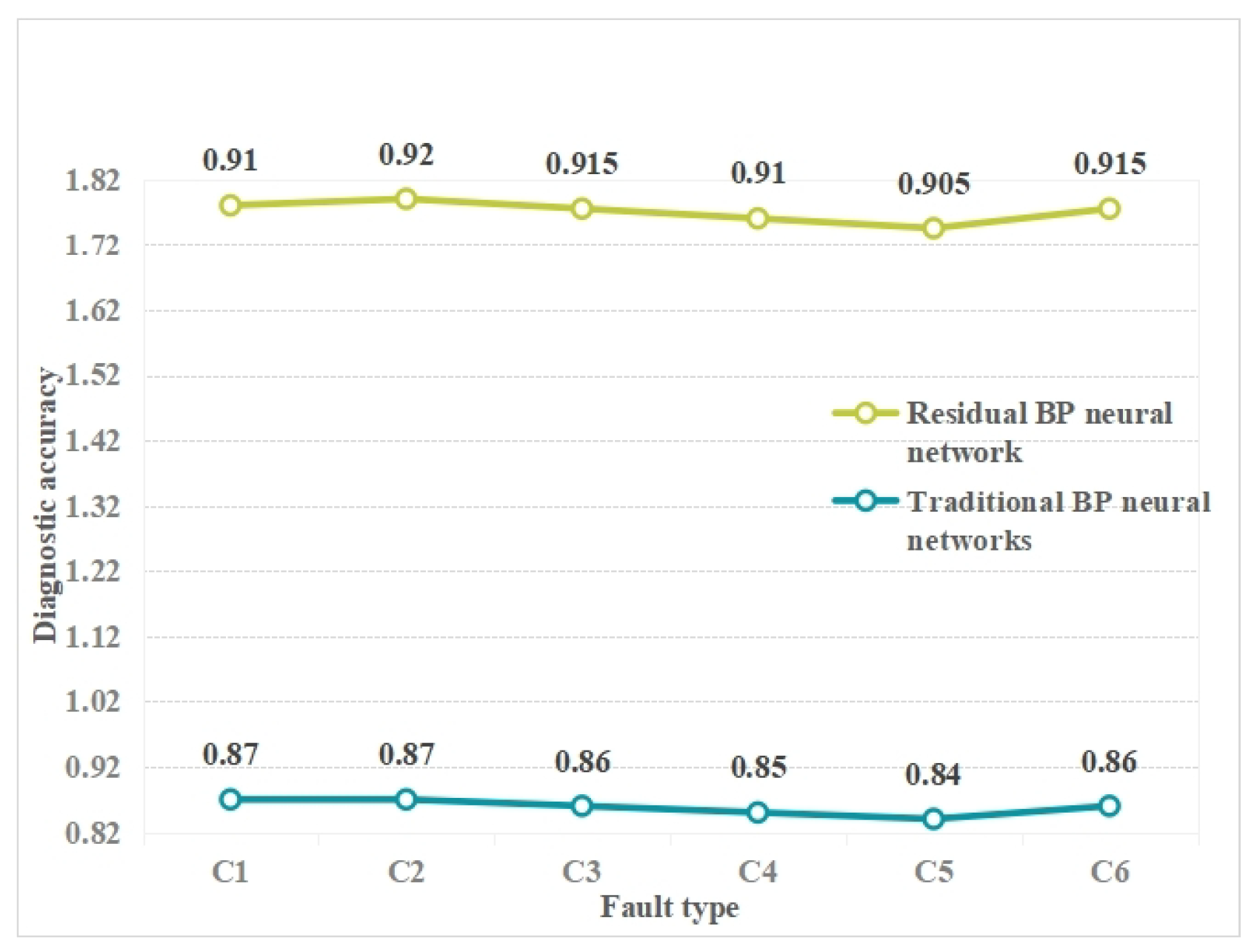
Figure 9 shows the improved accuracy of the residual BP neural network and the traditional deep BP neural network for the specific fault types of transformers in test set . As can be seen from Figure 9, among the six fault types of diagnosis, the diagnostic accuracy of the improved residual BP neural network model proposed in this paper is higher than that of traditional deep BP neural network.
In the diagnosis of different fault types, the improved residual BP neural network model has strong diagnostic stability, and the diagnostic accuracy of each fault type is maintained at above 90.9%. Table 14 shows the test results of some test data on the trained model. It can be seen from the table that the data of different fault types are tested, and the improved residual BP neural network model accurately predicts the type of corresponding fault data.
However, if IEC 60599 code, Duval triangle, and Rogers methods are used for diagnosis, there will be an incorrect diagnosis. Analyzing the error results, due to the different fault severities, occurrence points and causes, for transformers belonging to the same fault type, the dissolved gas content in the oil was shown to have a large difference, causing the samples to be classified into other fault types. The diagnostic model in this paper has a high diagnostic accuracy in the diagnostic results of the several transformer states shown above. At the same time, these methods have a limited ability to diagnose complex or multiple faults. Interpretation of the results requires expertise and experience. It is also relatively complex, requiring a lot of data collection and analysis. Interpretation may be subjective and depends on expert judgment. Therefore, the method used in this paper has certain advantages.
In order to comprehensively measure the superiority of the model proposed in this paper and avoid errors caused by the data, each model uses the same training set and test set to conduct 20 experiments; the actual diagnosis results are shown in Table 15. According to the diagnosis results of different models on the same data set, the diagnosis accuracy of the model is as high as 92%, which is higher than other algorithm models. Therefore, the model proposed in this paper can judge the state of the transformer very well.
During the process of data collection, there may sometimes be missed sampling or incorrect sampling. In order to prove that the model proposed in this paper still has a high diagnostic accuracy in the case of sampling errors, part of the data set was set to 10% wrong sampling. In this paper, the method of setting data to 0 was used to simulate the sampling error, and the fault diagnosis results are shown in Table 16.
Table 16 shows that the diagnostic accuracy of the model proposed in this paper declined when the sampling error of some data sets was considered, but the rate of decline was only 6%, while the diagnostic accuracy of other algorithms was lower than that of other algorithms. This significant drop indicates that the proposed model has strong robustness.
6. Discussion and Conclusions
This paper proposes a transformer fault diagnosis method that combines the residual backpropagation (BP) neural network with support vector machines (SVM), demonstrating an excellent performance in experiments. The aim was to enhance the reliability, operational efficiency, and energy utilization efficiency of the power grid, promote technological upgrades, provide a stable and reliable power supply, and contribute to sustainable economic and social development.
The method has the following characteristics: (a) After stacking multiple residual network modules, this method does not deepen the network layers, resulting in more accurate transformer fault diagnosis based on the residual BP neural network model. (b) Experimental results show that the proposed transformer fault diagnosis method, based on the improved residual BP neural network, outperforms the traditional deep BP neural network and shallow BP neural network diagnosis methods, and the proposed method maintains a good diagnostic performance with few sample data. (c) Interpolation methods are used to expand the positive and negative samples in the training and test sets, meeting the training requirements of the neural network, and enhancing the robustness and generalization performance of the network. By using the Euler distance coefficient and Pearson coefficient, as well as random sampling and data partitioning, the problem of insufficient learning with few sample data and excessive biased learning for with a large amount of sample data due to data imbalances can be alleviated. (d) The model is trained on a distributed computing platform, making it suitable for transformer fault type diagnosis with larger datasets.
Our research method employs a combined approach, using the residual backpropagation (BP) neural network and support vector machine (SVM) for transformer fault diagnosis. Many recent studies by experts in the field have also explored methods for diagnosing faults in power transformers. For instance, Liu Chang et al. [36] applied the bee algorithm to optimize the BP neural network for transformer fault diagnosis; Fu Baoying et al. [37] used the particle swarm algorithm to optimize the BP neural network for transformer fault diagnosis; Han Qingchun [38] proposed a transformer fault diagnosis method based on the cuckoo algorithm, optimizing the BP neural network; Zeng Zhi et al. [39] developed a transformer BP neural network fault diagnosis system based on the ant algorithm.
Researchers have employed various swarm intelligence algorithms, such as the bee algorithm, genetic algorithm, particle swarm algorithm, cuckoo algorithm, artificial fish swarm algorithm and ant algorithm, to optimize the BP neural network in studying transformer fault diagnosis techniques. These approaches have achieved results, but they also suffer from limitations and deficiencies in the iterative optimization process, including high computational complexity, a slow convergence speed, and susceptibility to local optima. As a consequence, these algorithms often lead to misdiagnoses when a transformer fault occurs, affecting the accuracy of transformer fault diagnosis.
Compared to these methods, the transformer fault diagnosis approach presented in this paper, which combines the residual backpropagation (BP) neural network with support vector machines (SVM), offers several advantages. The residual BP neural network enhances diagnostic accuracy by introducing residual learning. The improved combination of the residual BP neural network with SVM, through feature vector selection and weighting, demonstrates a better generalization performance under small sample data. Leveraging the deep feature learning ability of the residual BP neural network and the feature selection ability of SVM, our method can effectively handle complex fault scenarios, including low-probability faults and cross-impacts. By optimizing the model and adjusting parameters, our approach possesses high real-time and practical capabilities for practical applications. In the real-time monitoring and fault handling of power systems, rapid and accurate fault diagnosis is crucial, and our method meets this demand, ensuring the stability and safe operation of the power system.
However, when using our method, the acquisition of transformer fault data may be limited by the actual collection process and the frequency and types of transformer faults. Insufficient fault samples may affect the model’s generalization ability and robustness. The quality and scale of the dataset are critical to the method’s performance. Future research can explore the expansion of more real and diverse datasets and share these data with the academic and industrial communities to promote research and progress in this field.
When using SVM for feature vector evaluation and weight allocation in our method, appropriate parameter tuning may be necessary. Different parameter choices can impact the model’s performance; hence, further optimization and adjustments are required.
In the future, further research and applications of this method are necessary to continuously improve transformer fault diagnosis technology and drive the modernization of power systems. While this paper primarily focuses on fault diagnosis, in the future, the proposed method can be extended to the long-term operational health monitoring of transformers. Through real-time monitoring and diagnosis, potential faults can be better predicted, and preventive maintenance measures can be taken, thereby extending the life of transformers and increasing their reliability.
Author Contributions
Conceptualization, Y.J. and J.Z. (Jianfeng Zheng); methodology, Y.J., J.Z. (Jianfeng Zheng) and J.Z. (Ji Zhang); software, H.W.; validation, Z.L. and H.W.; formal analysis, H.W. and Y.J.; investigation, H.W.; resources, Y.J. and J.Z. (Jianfeng Zheng); data curation, Y.J. and H.W.; writing—original draft preparation, Y.J.; writing—review and editing, Y.J., J.Z. (Jianfeng Zheng) and J.Z. (Ji Zhang); visualization, Y.J.; supervision, Z.L. All authors have read and agreed to the published version of the manuscript.
Funding
This research received no external funding.
Institutional Review Board Statement
Not applicable.
Informed Consent Statement
Not applicable.
Data Availability Statement
Dataset link: https://github.com/jeson2017/TransformerFaultDiagnosisDataset.git (accessed on 30 May 2023).
Acknowledgments
I would like to express my heartfelt gratitude to many people who helped during the process of completing this study. Their help, support, and encouragement played an important role in my completing this work. In addition, I would like to thank the members of the laboratory. They have provided me with a lot of help in the operation of experimental equipment and data collection. Their cooperation and teamwork spirit have enabled my research to proceed smoothly.
Conflicts of Interest
The authors declare no conflict of interest.
Abbreviations
The following abbreviations are used in this manuscript:
| BP | Back Propagation |
| DGA | Dissolved Gas Analysis |
| SVM | Support Vector Machine |
| IEC | International Electrotechnical Commission |
| Bi-LSTM | Bi-directional Long Short-Term Memory |
References
- Equbal, M.; Khan, S.A.; Islam, T. Transformer incipient fault diagnosis on the basis of energy-weighted DGA using an artificial neural network. Turk. J. Electr. Eng. Comput. 2018, 26, 77–88. [Google Scholar] [CrossRef]
- Wang, D.; Lei, Q. Fault diagnosis of power transformer based on BR-DBN. Electr. Power Autom. Equip. 2018, 38, 129–135. [Google Scholar]
- Maofa, G.; Yanni, L.; Laihe, W.; Baoye, S.; Wenqiang, Z. Fault diagnosis of power transformers based on chaos particle swarm optimization BP neural network. Electr. Meas. Instrum. 2016, 53, 13–16. [Google Scholar]
- Feng, Z.; Shuo, L. Fault Diagnosis of Traction Transformer Based on DGA and Improved Association Degree Model. High Volt. Appar. 2015, 51, 41–45. [Google Scholar]
- Zhang, W.; Yuan, J.; Zhang, T.; Zhang, K. An improved three-ratio method for transformer fault diagnosis using B-spline theory. Proc. CSEE 2014, 34, 4129–4136. [Google Scholar]
- Yang, X.; Chen, W.; Li, A.; Yang, C.; Xie, Z.; Dong, H. BA-PNN-based methods for power transformer fault diagnosis. Adv. Eng. Inform. 2019, 39, 178–185. [Google Scholar] [CrossRef]
- Weihua, Z.; Jinsha, Y.; Shan, W. A caculation method for transformer fault basic probability assignment based on improved three-ratio method. Power Syst. Prot. Control 2015, 43, 115–121. [Google Scholar]
- Li, Y.; Shu, N. Transformer fault diagnosis based on fuzzy clustering and complete binary tree support vector machine. Trans. China Electrotech. Soc. 2016, 31, 64–70. [Google Scholar]
- Kari, T.; Gao, W.; Zhao, D.; Abiderexiti, K.; Mo, W.; Wang, Y.; Luan, L. Hybrid feature selection approach for power transformer fault diagnosis based on support vector machine and genetic algorithm. IET Gener. Transm. Distrib. 2018, 12, 5672–5680. [Google Scholar] [CrossRef]
- Yuan, F.; Guo, J.; Xiao, Z. A transformer fault diagnosis model based on chemical reaction optimization and twin support vector machine. Energies 2019, 12, 960. [Google Scholar] [CrossRef]
- Xiao, Y.; Pan, W.; Guo, X.; Bi, S.; Lin, S. Fault Diagnosis of Traction Transformer Based on Bayesian Network. Energies 2020, 13, 4966. [Google Scholar] [CrossRef]
- Zeng, B.; Guo, J.; Zhu, W.; Xiao, Z.; Yuan, F.; Huang, S. A Transformer Fault Diagnosis Model Based On Hybrid Grey Wolf Optimizer and LS-SVM. Energies 2019, 12, 4170. [Google Scholar] [CrossRef]
- Yang, Z. “Guidelines for Dissolved Gas Analysis and Fault Diagnosis of Transformers”—A Discussion on Transformer Fault Diagnosis. Transformer 2008, 45, 24–27. [Google Scholar]
- Zhu, Y.; Yin, J. Study on application of multi-kernel learning relevance vector machines in fault diagnosis of power transformers. IEEE Inst. Electr. Electron. Eng. 2013, 33, 68–74. [Google Scholar]
- Hanbo, Z.; Wei, W.; Xiaogang, L.; Linan, W.; Yuquan, L.; Jinhua, H. Fault diagnosis method of power transformers using multi-class LS-SVM and improved PSO. High Volt. Eng. 2014, 40, 3424–3429. [Google Scholar]
- Shijun, H.; Ju, Z.; Jigui, M. Fault Diagnosis of Transformer Based on Particle Swarm Optimization-Based Support Vector Machine. Electr. Meas. Instrum. 2014, 51, 71–75. [Google Scholar]
- Ali, M.S.; Abu Bakar, A.H.; Omar, A.; Abdul Jaafar, A.S.; Mohamed, S.H. Conventional methods of dissolved gas analysis using oil-immersed power transformer for fault diagnosis: A review. Electr. Power Syst. Res. 2023, 216, 109064. [Google Scholar] [CrossRef]
- Taha, I.; Hoballah, A.; Ghoneim, S. Optimal Ratio Limits of Rogers’ Four-Ratios and IEC 60599 Code Methods Using Particle Swarm Optimization Fuzzy- Logic Approach. IEEE Trans. Dielectr. Electr. Insul. 2020, 27, 222–230. [Google Scholar] [CrossRef]
- Deng, X.; Zhu, H.; Liu, S. Research on Digital Twin Modeling Technology for Transformer Protection. Power Syst. Technol. 2022, 46, 4982–4992. [Google Scholar]
- Yuan, J.; Xu, P.; Li, L. Prediction of transformer oil- paper insulation aging based on BP neural networks with the chicken swarm optimization algorithm. J. Electr. Power Sci. Technol. 2020, 35, 33–41. [Google Scholar]
- Wang, B.; Yang, Y.; Zhang, S. Fault diagnosis of support vector machine transformer based on improved BP neural network. Electr. Meas. Instrum. 2019, 56, 53–58. [Google Scholar]
- Li, P.; Hu, G. Transformer fault diagnosis method based on the fusion of improved neural network and ratio method. High Volt. Eng. 2022, 7, 1–9. [Google Scholar] [CrossRef]
- Xu, X.; Jiang, B.; Cao, W. Application of locust optimized neural network in transformer fault diagnosis. Power Syst. Clean Energy 2021, 37, 17–23. [Google Scholar]
- Xian, R.; Fan, H.; Li, F. Power Transformer Fault Diagnosis Based on Improved GSA-SVM Model. Smart Power 2022, 50, 50–56. [Google Scholar]
- Xiong, Y.; Liao, X.; Ke, F. Life cycle cost analysis of main transformer based on the multi-system data fusion. J. Electr. Power Sci. Technol. 2020, 35, 3–11. [Google Scholar]
- Fu, H.; Ren, R.; Yan, Z.; Ma, Y. Fault Diagnosis Method of Power Transformers Using Multi-kernel RVM and QPSO. Gaoya Dianqi/High Volt. Appar. 2017, 53, 131–135+141. [Google Scholar]
- Song, Z.J.; Wang, J. Transformer Fault Diagnosis Based on BP Neural Network Optimized by Fuzzy Clustering and LM Algorithm. High Volt. Appar. 2013, 49, 54–59. [Google Scholar]
- Li, X.; Chen, Z.; Fan, X. Fault Diagnosis of Transformer Based on BP Neural Network and ACS-SA. High Volt. Appar. 2018, 54, 134–139+146. [Google Scholar]
- Yuan, P.; Mao, J.; Xiao, F. Grid Fault Diagnosis Based on Improved Genetic Optimization BP Neural Network. J. Electr. Power Syst. Autom. 2017, 29, 118–122. [Google Scholar]
- Wu, R.; Li, C. Design of Transformer Fault Intelligent Diagnosis System. In Proceedings of the 2021 International Conference on Networking Systems of AI (INSAI), Shanghai, China, 19–20 November 2021; pp. 293–296. [Google Scholar] [CrossRef]
- Zhao, W. Study for Transformer Fault Diagnosis and Forecast Based on Data Mining. Master’s Thesis, North China Electric Power University, Beijing, China, 2009. [Google Scholar]
- Huang, Y.; Huang, S. Condition Maintenance of Power Generation Equipment; China Power Press: Beijing, China, 2000. [Google Scholar]
- Du, J. Transformer Fault Diagnosis Expert System. Master’s Thesis, North China Electric Power University, Beijing, China, 2003. [Google Scholar]
- Crowley, T.H.; Hagman, W.H.; Tabors, R.D.; Cooke, C.M. Expert system for on-line monitoring of large power transformers. Expert Syst. Appl. Electr. Power Ind. 1990, 1, 629–660. [Google Scholar]
- Yin, J. Research on Fault Diagnosis Method of Oil-immersed Power Transformers Based on Correlation Vector Machine. Ph.D. Thesis, North China Electric Power University, Beijing, China, 2013. [Google Scholar]
- Liu, C.; Wu, J.; Gao, Y. Transformer Fault Diagnosis Based on BP Neural Network and Bee Colony Algorithm. Industrialization 2020, 10, 7–11. [Google Scholar]
- Fu, B.; Wng, Q. Transformer fault diagnosis based on adaptive Particle swarm optimization BP neural network. J. Huaqiao Univ. 2013, 34, 262–266. [Google Scholar]
- Han, Q. Research on Transformer Fault Diagnosis Based on the Optimization of BP Neural Network Using the Bouguebird Algorithm. Master’s Thesis, Shandong University of Science and Technology, Qingdao, China, 2019. [Google Scholar]
- Zeng, Z.; Zhang, H.; Yang, T.; Zeng, X.; Zeng, C. Power transformer incipient fault diagnosis based on neural network optimized by combined ant colony optimization. Electrotech. Appl. 2019, 38, 43–49. [Google Scholar]
Figure 1.
Transformer fault diagnosis method.

Figure 2.
Schematic diagram of a support vector machine.

Figure 3.
Residual Network Module.

Figure 4.
Improved model of neural network.
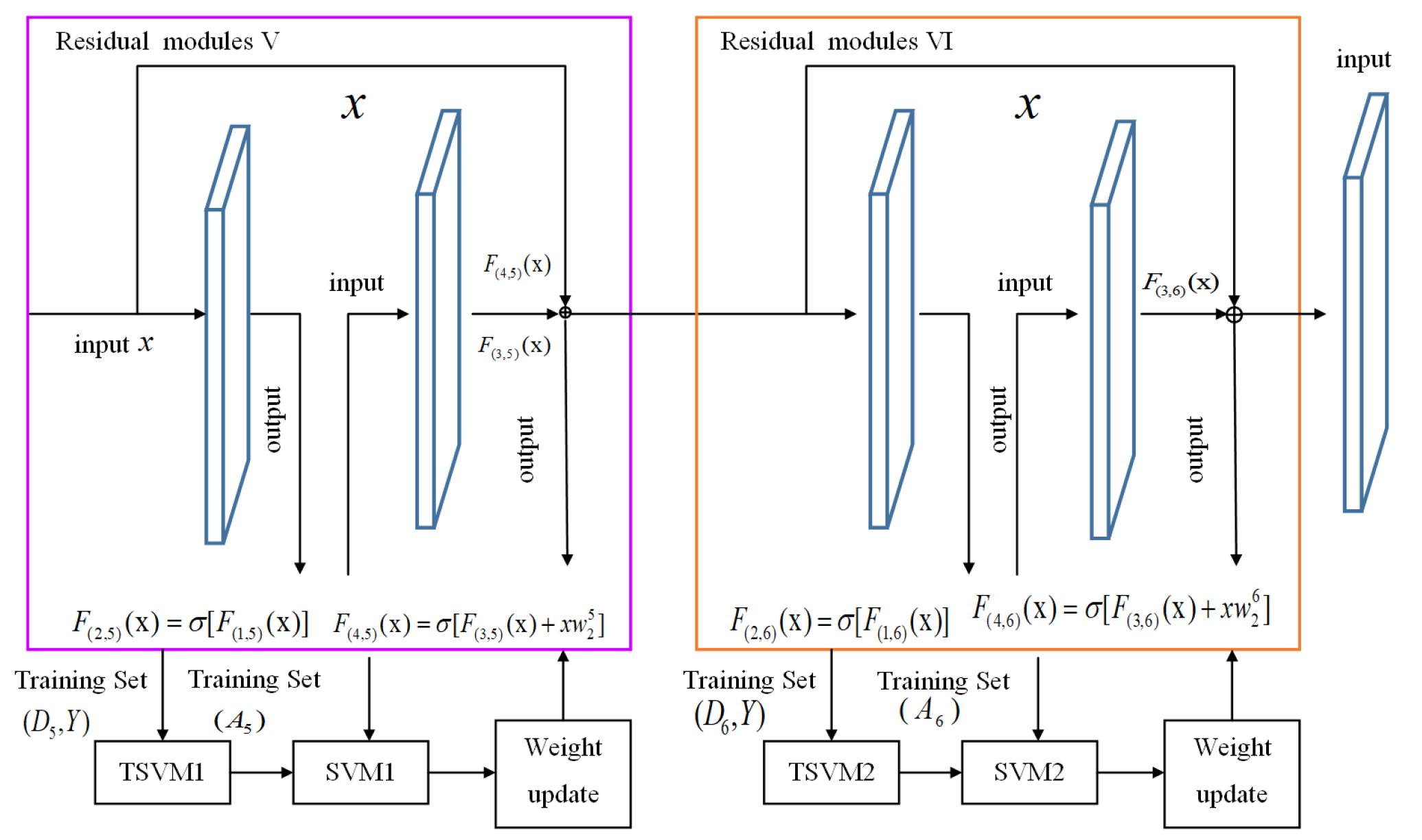
Figure 5.
Cubic Hermita polynomial interpolation.
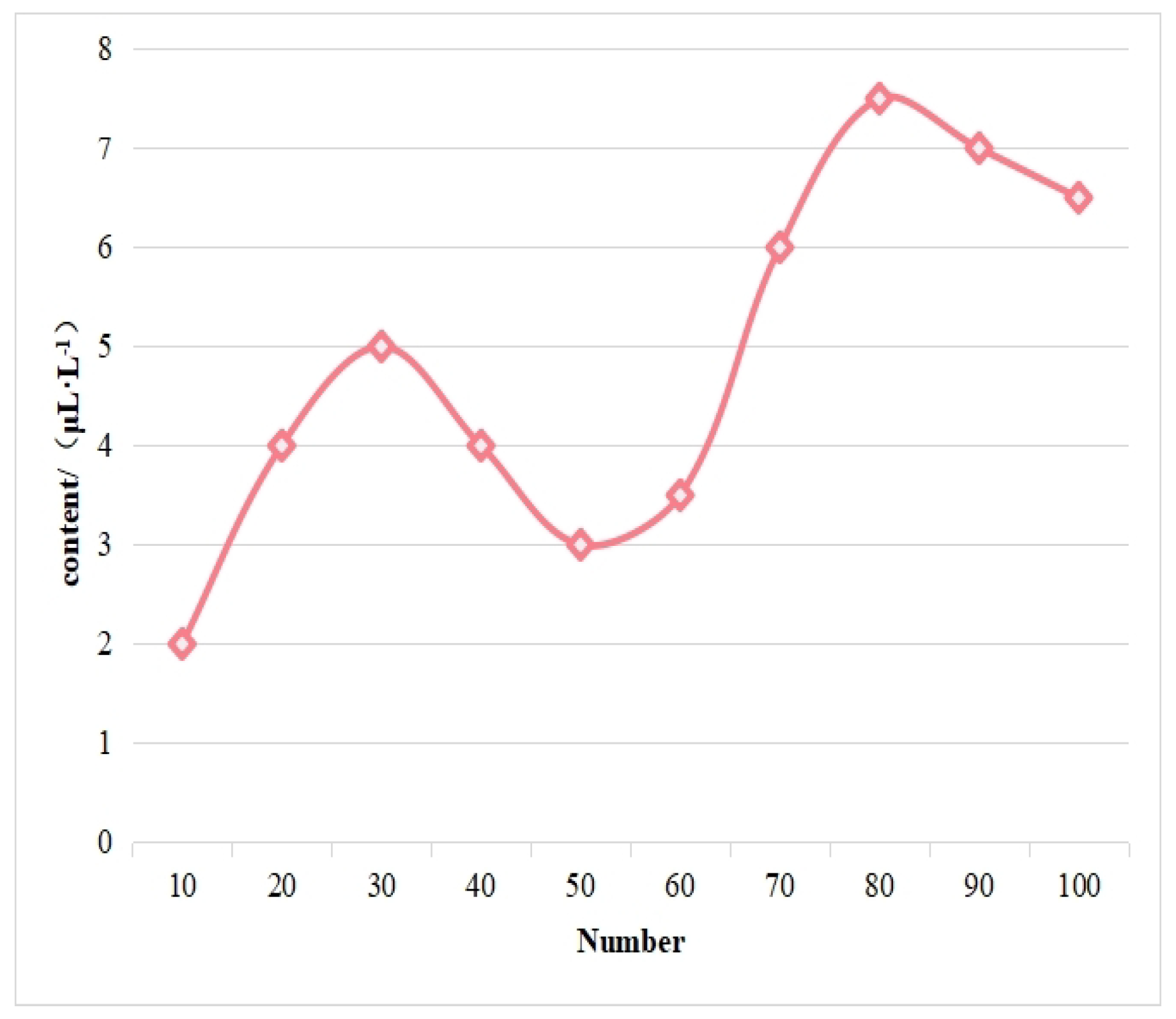
Figure 6.
Training process of the improved BP neural network.
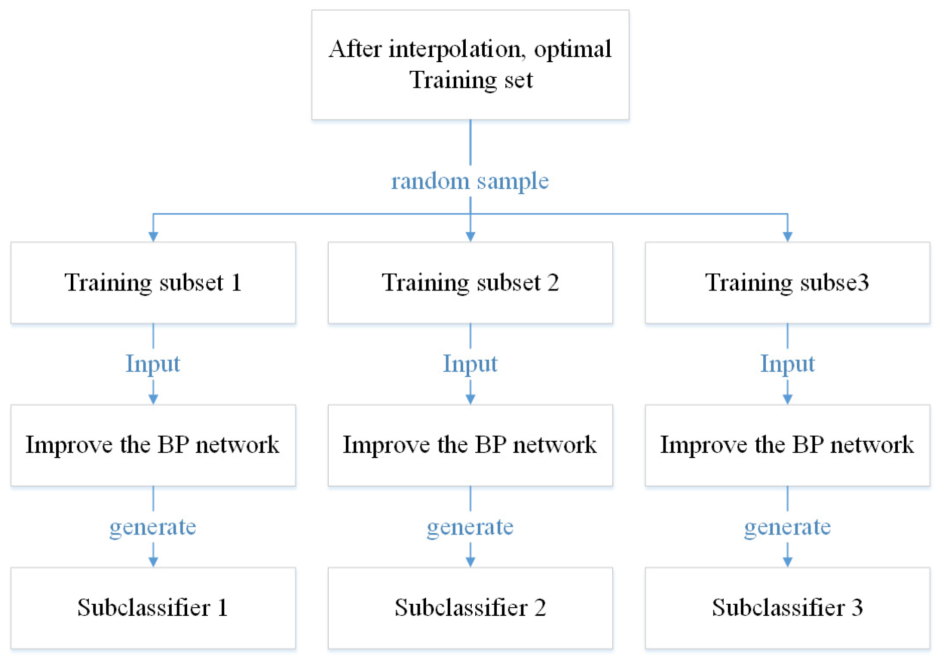
Figure 7.
Diagnostic process of the improved BP neural network.
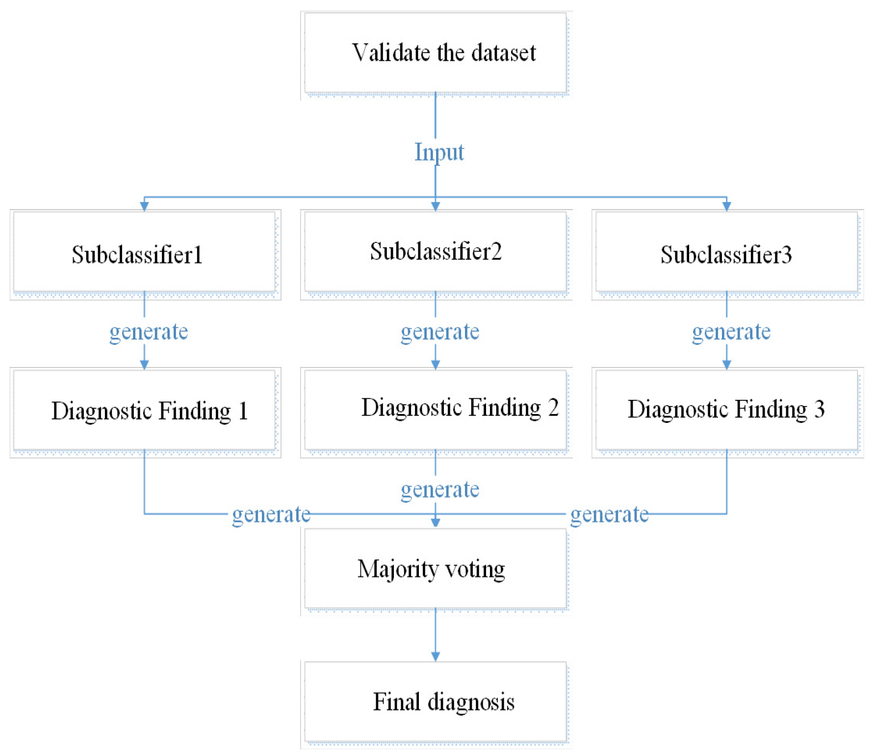
Figure 8.
Confusion matrix.
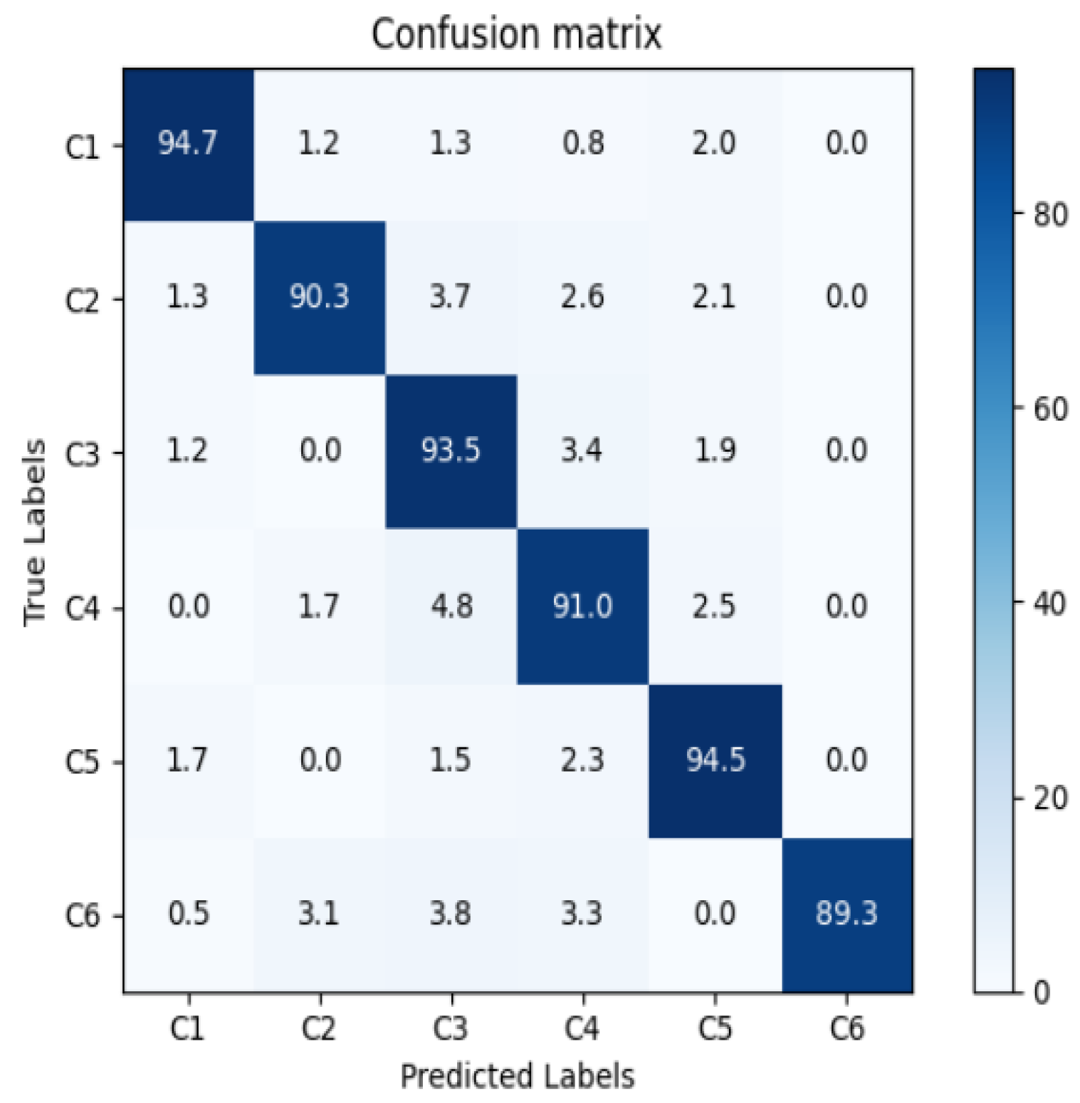
Figure 9.
Diagnostic results of transformer fault types.

Table 1.
Typical faults of power transformers.
| Fault Type | Cause |
|---|---|
| Low-temperature overheating (≤300 ) | The output of the transformer exceeds the rated value, causing the core temperature to rise rapidly; The transformer cooling device does not work properly; The ambient temperature rises or the ambient temperature around the transformer rises, or the environment around the transformer is not conducive to heat dissipation. |
| Medium- temperature overheating (300 –700 ) | Medium-temperature overheating (300 –700 ) |
| High-temperature overheating (>700 ) | Insufficient pressure of electric shock; There is an oil sludge film between the dynamic and static contacts; Burns on the contact surface; Mechanical damage to insulation during manufacturing; Insulation aging or debris in the oil, blocking the oil passage and causing high-temperature damage to the insulation; Through-the-loop short-circuit fault joint heat, due to the insulation damage of the pressure ring screw or the pressure ring contact touching the iron core. Due to the circulating current, magnetic leakage makes the iron parts eddy current larger. |
| Partial discharge | The air humidity around the transformer is too large, and the insulation of some areas of the transformer body is not strong enough, or the transformer insulation is damaged during installation, resulting in partial discharge of the transformer; The oil level of the transformer drops, causing the live parts inside the transformer to not be covered by the insulating oil, resulting in partial discharge of the transformer. |
| Low-energy discharge | There are more impurities in oil-immersed transformer oil that cause low-energy discharge; The metal parts inside the transformer are disconnected due to poor manufacturing, transportation, installation technology, etc., and the levitation potential causes low-energy discharge. |
| High-energy discharge | Coil-to-turn insulation breakdown; Overvoltage causes internal flashover; arcing caused by lead breakage; Tap changer arcing and capacitive screen breakdown. |
Table 2.
Gas content limit values.
| Gas Composition | Ethylene | Ethane | Acetylene | Methane | Total Hydrocarbons | |
|---|---|---|---|---|---|---|
| Critical value | 150 | 65 | 35 | 5 | 45 | 150 |
Table 3.
Critical values for gas production rates.
| Gas Composition | Closed (mL/d) | Open (mL/d) |
|---|---|---|
| Total hydrocarbons | 12 | 6 |
| Acetylene | 0.2 | 0.1 |
Table 4.
Transformer faults and corresponding gases.
| Fault Type | Main Ingredients | Minor Gas Components |
|---|---|---|
| The insulating oil is overheated | , | , |
| Teinsulatin Oylis Ofheited | , , | , , |
| Insulating oil and paper arc discharge | , , , | , , |
| Arc discharge in insulating oil | , , | , |
| Akdi Shegin in Suratingil | , , | , , |
| Low energy discharge in insulating oil | , |
Table 5.
Oerswald coefficient of gases in transformer oil.
| Standard | Temperature | |||||||
|---|---|---|---|---|---|---|---|---|
| GB/T17623.1998 | 50 | 0.06 | 0.12 | 0.92 | 0.39 | 1.02 | 1.46 | 2.3 |
| IEC60599.1999 | 50 | 0.05 | 0.12 | 1 | 0.4 | 0.9 | 1.4 | 1.8 |
Table 6.
Relationship between transformer fault types and characteristic gases.
| Serial Number | Nature of the Failure | Characteristic Gas Characteristics |
|---|---|---|
| 1 | General overheating failure | Total hydrocarbons are too high, < 5 L/L |
| 2 | Severity overheating failure | high total hydrocarbons > 5 L/L, However, did not constitute the main component of total hydrocarbons, and the content was high |
| 3 | Partial discharge | Total hydrocarbons are not high, >100 L/L, This accounts for the main component of total hydrocarbons |
| 4 | Patialdi | Total hydrocarbons are not high, > 10 L/L, Totahid Rocabens–Anotte Sea |
| 5 | Arcing | The total hydrocarbon content is high, the content is high, and the content is high, but it is not the main component |
Table 7.
Coding rules of the three-ratio method.
| Gas Ratio Range | Ratio Encoding Range | ||
|---|---|---|---|
| / | / | ||
| <0.1 | 0 | 1 | 0 |
| ≥0.1∼<1 | 1 | 0 | 0 |
| ≥1∼<3 | 1 | 2 | 1 |
| ≥3 | 2 | 2 | 2 |
Table 8.
Troubleshooting without coding ratio method.
| Nature of the Failure | Typical Example | |||
|---|---|---|---|---|
| Low-temperature overheating (<300 ) | <0.1 | Independent | <1 | The winding oil passage is blocked, and the iron core is short-circuited |
| Medium-temperature overheating | <0.1 | Independent | 1<ratio<3 | Tap changer lead connector contact |
| (300–700 ) | Poor, iron core multi-point grounding bureau | |||
| High-temperature overheating (>) | <0.1 | Independent | >3 | Local short circuit |
| High-energy discharge | 0.1 < ratio < 3 | <1 | Independent | Short-circuit circumference between winding turns and cake rooms, screen discharge, load tap and switch |
| High-energy discharge and overheating | 0.1 < ratio < 3 | >1 | Independent | The selector switch cuts off the current |
| Low-energy discharge | >3 | <1 | Independent | Fence dendritic discharge, tap |
| Low-energy discharge and overheating | >3 | >1 | Independent | The switch is misaligned, and the selector switch is not in place |
Table 9.
Comparison of common methods for transformer fault diagnosis.
| Algorithm | Peculiarity |
|---|---|
| Characteristic gas method | This can visually determine whether there is a latent fault, but cannot determine the type and status of the fault |
| Ratio method | Simple and convenient, but the encoding will be missing, and the coding information corresponding to the fault state cannot be found |
| Fuzzy theory | This can better deal with the uncertainty and ambiguity between fault types and symptoms, but can determine the membership function based on experience. Rhere is more human intervention, and there is a lack of a convincing objective basis |
| Expert system | A large amount of experimental data and monitoring information can be comprehensively evaluated and analyzed, but expert knowledge is difficult to express in rules, and the reasoning of expert systems has some uncertainties |
| Support vector machine | This is mainly used for binary classification problems, and is not effective for multi-classification problems |
| BP neural network | There is a clear input–output relationship, and it has a good effect in multi-classification |
Table 10.
Transformer Status Codes.
| Transformer Status | Encode |
|---|---|
| normal | (1,0,0,0,0,0) |
| Low-energy discharge | (0,1,0.0.0.0) |
| High-energy discharge | (0,0,1,0.0.0) |
| Medium- and low-temperature overheating | (0,0,0,1,0,0) |
| High-temperature overheating | (0,0,0,0,1,0) |
| Partial discharge | (0,0,0,0.0,1) |
Table 11.
Ablation experiment results.
| Model | SVM | Residual Network Module | Precision/% |
|---|---|---|---|
| BP neural network | × | × | 87.2 |
| ✓ | × | 91.3 | |
| × | ✓ | 89.8 | |
| ✓ | ✓ | 92.7 |
“×” means that this module is not added to the network model, while “✓” means that this module is added to the network model.
Table 12.
Diagnostic accuracy of different models.
| Model | Test Set Diagnostic Accuracy/% | Average Diagnostic Accuracy/% | ||
|---|---|---|---|---|
| Improved residual BP neural network | 91.52 | 92.26 | 93.75 | 92.51 |
| Traditional shallow BP neural networks | 87.94 | 88.69 | 90.18 | 89.94 |
| Traditional deep BP neural networks | 86.16 | 86.90 | 87.50 | 86.85 |
Table 13.
Diagnostic accuracy of different models with few sample data.
| Model | Test Set Diagnostic Accuracy/% | Average Diagnostic Accuracy/% | ||
|---|---|---|---|---|
| Improved residual BP neural network | 91.07 | 90.18 | 89.88 | 90.38 |
| Traditional shallow BP neural networks | 85.71 | 84.82 | 83.33 | 84.62 |
| Traditional deep BP neural networks | 83.93 | 83.03 | 82.74 | 83.23 |
Table 14.
Shows some of the test data tables.
| Serial Number | Gas Content/(L/L) | The Actual Failure Type | Predict the Result (Ours) | IEC_60599 | Duval Triangle | Rogers Methods | ||||
|---|---|---|---|---|---|---|---|---|---|---|
| 1 | 14.67 | 3.68 | 10.54 | 2.71 | 0.2 | normal | ||||
| 2 | 27 | 90 | 42 | 63 | 0.2 | Medium and low temperature overheating | ||||
| 3 | 73 | 12.3 | 3.33 | 27.1 | 47.9 | Partial discharge | ||||
| 4 | 135 | 466 | 70 | 502 | 9 | High temperature overheating | ||||
| 5 | 119 | 25 | 12 | 55 | 84 | High energy discharge | ||||
| 6 | 80 | 20 | 6 | 20 | 62 | Low energy discharge | ||||
Table 15.
Comprehensive accuracy of each algorithm.
| Algorithm | Correct Rate (%) |
|---|---|
| SVM | 85 |
| Bi-LSTM | 89 |
| Traditional BP neural network | 87 |
| Our method | 92 |
Table 16.
Comparison of comprehensive accuracy under the data set with errors.
| Algorithm | Model Diagnostic Accuracy (\%) | Average Percentage (%) | |
|---|---|---|---|
| Dataset Is Error-Free | Dataset Error | ||
| SVM | 85 | 73 | 12 |
| Bi-LSTM | 89 | 72 | 17 |
| Traditional BP neural network | 87 | 71 | 16 |
| Our method | 92 | 86 | 6 |
Disclaimer/Publisher’s Note: The statements, opinions and data contained in all publications are solely those of the individual author(s) and contributor(s) and not of MDPI and/or the editor(s). MDPI and/or the editor(s) disclaim responsibility for any injury to people or property resulting from any ideas, methods, instructions or products referred to in the content. |
© 2023 by the authors. Licensee MDPI, Basel, Switzerland. This article is an open access article distributed under the terms and conditions of the Creative Commons Attribution (CC BY) license (https://creativecommons.org/licenses/by/4.0/).
Share and Cite
MDPI and ACS Style
Jin, Y.; Wu, H.; Zheng, J.; Zhang, J.; Liu, Z. Power Transformer Fault Diagnosis Based on Improved BP Neural Network. Electronics 2023, 12, 3526. https://doi.org/10.3390/electronics12163526
AMA Style
Jin Y, Wu H, Zheng J, Zhang J, Liu Z. Power Transformer Fault Diagnosis Based on Improved BP Neural Network. Electronics. 2023; 12(16):3526. https://doi.org/10.3390/electronics12163526
Chicago/Turabian StyleJin, Yongshuang, Hang Wu, Jianfeng Zheng, Ji Zhang, and Zhi Liu. 2023. "Power Transformer Fault Diagnosis Based on Improved BP Neural Network" Electronics 12, no. 16: 3526. https://doi.org/10.3390/electronics12163526
Note that from the first issue of 2016, this journal uses article numbers instead of page numbers. See further details here.