A Hybrid Method of Adaptive Cross Approximation Algorithm and Chebyshev Approximation Technique for Fast Broadband BCS Prediction Applicable to Passive Radar Detection

Abstract

A hybrid method combining the adaptive cross approximation method (ACA) and the Chebyshev approximation technique (CAT) is presented for fast wideband BCS prediction of arbitrary-shaped 3D targets based on non-cooperative radiation sources. The incident and scattering angles can be computed by using their longitudes, latitudes and altitudes according to the relative positions of the satellite, the target and the passive bistatic radar. The ACA technique can be employed to reduce the memory requirement and computation time by compressing the low-rank matrix blocks. By exploiting the CAT into ACA, it is only required to calculate the currents at several Chebyshev–Gauss frequency sampling points instead of direct point-by-point simulations. Moreover, a wider frequency band can be obtained by using the Maehly approximation. Three numerical examples are presented to validate the accuracy and efficiency of the hybrid ACA-CAT method.

1. Introduction

In recent years, passive bistatic radars (PBRs) have been developed rapidly. PBRs have many advantages. First, since they do not radiate electromagnetic waves into space, PBRs have stealthy characteristics. Secondly, PBRs can make extensive use of the non-cooperative sources of radio energy, including radar signals [1], digital audio/video signals [2,3], navigation signals [4], frequency-modulated radio signals [5,6], television signals [7] and even mobile communication signals [8,9]. PBRs’ capacity for target detection and recognition is also addressed through the use of a new cooperative satellite transmitter [10,11,12,13]. Thus, PBRs have the advantage of flexibility in receiving signals. Finally, passive radars are generally low-cost, as they only need a receiver which can be easily found on the commercial market.

Since antennas in communications, navigation and broadcasting applications operate at a frequency range from C band to Ka band, we need to predict the bistatic cross-section (BCS) over a broad frequency band. The method of moments is widely used for the analysis of electromagnetic scattering and radiation problems. However, the memory requirement of impedance matrix and computational complexity based on an iterative solver is O(N²) and O(N²), respectively, where N is the number of unknowns. Moreover, the traditional method of moments needs to calculate the currents at each frequency point and this process is very time-consuming, which makes it impossible to obtain the broadband radar cross-section (RCS) quickly.

To overcome the shortcomings of traditional MoM, various fast computational methods have emerged. These fast methods based on MoM have been proposed to reduce the memory requirement and accelerate the matrix–vector products (MVPs), including the Fast Multipoles Method (FMM) [14,15,16,17,18], the Multilevel Fast Multipoles Algorithm (MLFMA) [17,18], the Adaptive Integral Method (AIM) [19,20], Integral Equation-Fast Fourier Transform (IE-FFT) [21] and so on. The Fast Multipole Method (FMM) was proposed as an augmentation of the Method of Moments, which allows the calculation of electrically large problems, and the Multilevel Fast Multipole Algorithm (MLFMA) can further improve the computational efficiency. The memory requirement and computational complexity of MLFMA are O(N) and O(NlogN), respectively. The AIM and IE-FFT can accelerate the matrix vector multiplication by using FFT and avoid storing the impedance matrix elements directly. The required memory can be reduced to O(N), and the computational complexity can be reduced to O(kNlogN); however, it is more suitable for volume fractional equations and less effective for surfaces.

Adaptive cross approximation (ACA)-based [22,23,24] methods are fully algebraic and kernel-independent. They are easily inserted into existing MoM codes. The ACA method adaptively constructs compressed blocks by using only some matrix elements with no further problem-related information. The ACA is a rank-revealing matrix decomposition method which has received widespread attention in the computational electromagnetics community. For analyzing moderate electrical size targets, the ACA algorithm can reduce the memory requirement and computational complexity of the MoM to O(N^4/3logN) and O(NlogN), respectively.

Satellite antennas in communications [25], navigation and broadcasting applications operate at a frequency range from C band to Ka band. Therefore, if we use these satellite signals as transmitters, we need to achieve RCS prediction over a wide frequency range. However, the ACA needs to solve the integral equation at each frequency point, resulting in extensive computation time.

To alleviate this difficulty, many model order reduction (MOR) techniques, such as the asymptotic waveform evaluation (AWE) technique [26,27], the impedance matrix interpolation technique [28], the Cauchy method and the Chebyshev approximation technique (CAT) [29,30], have been proposed for fast frequency sweep analysis. Among the aforementioned techniques, the AWE technique has been successfully applied in various electromagnetic problems. Besides, it can be easily incorporated with the Finite Element Method (FEM) [31], the Finite Element–Boundary Integral Method (FE-BI) [32], Pre-Corrected FFT [33] and the Adaptive Integral Method (AIM). However, the high-order derivatives of the impedance matrix and excitation vector must be calculated and stored, leading to a high memory cost. Compared to the AWE, the CAT is much more convenient to integrate into the ACA code since it does not need to store and solve the large derivatives of impedance matrices.

In this paper, a novel hybrid ACA-CAT technique is proposed for fast wideband RCS computation of arbitrary-shaped 3D targets. In the ACA approach, the impedance matrix is divided into near-field and far-field blocks, and the far-field impedance blocks are compressed into low-rank matrix blocks. The ACA, which can reduce the memory storage and accelerate the matrix–vector products, are employed to calculate the currents at Chebyshev–Gauss sampling points. By using the proposed hybrid ACA-CAT, the current at any frequency point over the whole broadband can be obtained. Compared to the direct point-by-point ACA-MoM solutions, the ACA-CAT can greatly reduce computational costs without loss of accuracy.

The remainder of this paper is organized as follows. Section 2 reviews fundamentals of the MoM of arbitrary-shaped 3D targets based on non-cooperative satellite-borne illuminators. The formula and solution procedure of the proposed ACA-CAT algorithm are given in Section 3. Three examples are presented in Section 4 to verify the accuracy and efficiency of the hybrid ACA-CAT algorithm. Section 5 concludes the main outcomes of this paper and gives a brief introduction to some other applications for the hybrid method.

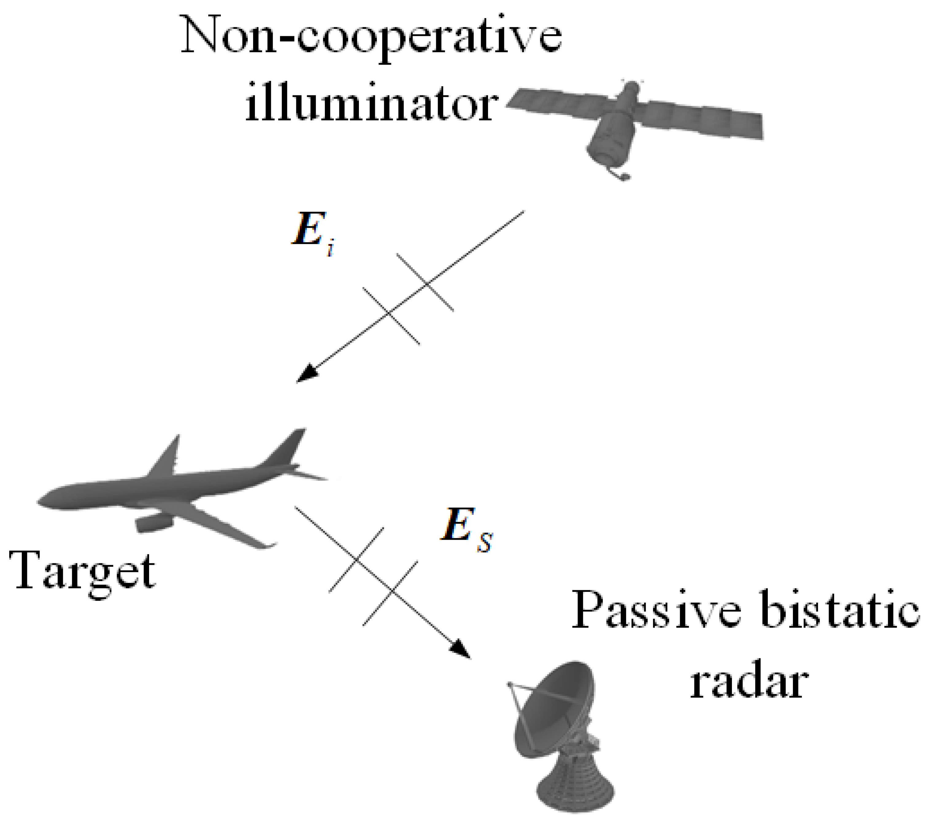
2. The MoM Based on Non-Cooperative Satellite-Borne Illuminator

The MoM is able to solve the problem of electromagnetic scattering by transforming the corresponding integral equation into a matrix equation. We consider a perfect conductor target illuminated by a broadband non-cooperative satellite source, and the scattered signal due to the scattering of the target is received by the passive bistatic radar on the ground, as shown in Figure 1.

The electric field integral equation (EFIE) can be written as:

$${\left[E^i\left(r\right)\right]|}_t={\left\{jk\eta {\displaystyle {\iint }_S\left[J\left(r^{\prime }\right)G\left(r,r^{\prime }\right)+\frac{1}{k^2}\nabla {\nabla }^{\prime }\cdot J\left(r^{\prime }\right)G\left(r,r^{\prime }\right)\right]d{r}^{\prime }}\right\}|}_t$$

(1)

where $E^i\left(r\right)$ denotes the incident plane wave, $J\left(r\right)$ represents the surface current, k represents the wave number at a certain frequency f, η denotes the free-space intrinsic impedance, and $G\left(r,r^{\prime }\right)$ is Green’s function.

Using the triangle to mesh the surface of the target, the current on the surface of the target is expanded by the RWG basis function $f_n\left(r\right)$, $(n=1,2\dots ,N)$:

$$J\left(r\right)={\displaystyle \sum _{n=1}^N{I}_n{f}_n\left(r\right)}$$

(2)

where $N$ is the number of basis functions and $I_n$ is the unknown coefficient.

By substituting (2) into (1), the inner product of the electric field integral equation using the Galerkin method can be expressed in a vector form, and then a matrix equation can be obtained as:

$$ZI=V$$

(3)

where $I$ denotes unknown current density. The elements of the impedance matrix $Z$ and the excitation vector $V$ can be calculated as:

$$\begin{array}{l}{Z}_{mn}=jk\eta \{{\displaystyle {\iint }_{f_m}{f}_m\left(r\right)\cdot {\displaystyle {\iint }_{f_n}{f}_n\left(r^{\prime }\right)}G\left(r,r^{\prime }\right)d{r}^{\prime }dr}\\ \hspace{1em}\hspace{1em}+\frac{1}{k^2}{\displaystyle {\iint }_{f_m}{f}_m\left(r\right)\cdot \left[\nabla {\displaystyle {\iint }_{f_n}{\nabla }^{\prime }\cdot f_n\left(r^{\prime }\right)}G\left(r,r^{\prime }\right)d{r}^{\prime }\right]dr}\}\end{array}$$

(4)

$$V_m={\displaystyle {\iint }_{f_m}{f}_m\left(r\right)\cdot E^i\left(r\right)dr}$$

(5)

where $\eta =\sqrt{{\mu }_0/{\epsilon }_0}$ represents the free-space intrinsic impedance. $r^{\prime }$ and $r$ denote the source and field points, respectively. $f_m\left(r\right)$, $(m=1,2\dots ,N)$ and $f_n\left(r^{\prime }\right)$ are the basis and test functions, respectively.

In (1), $E^i$ represents the electric field of an arbitrary plane wave, which can be given by:

$$E^i\left(k,r\right)=\left(E_{\theta }\widehat{\theta }+E_{\phi }\widehat{\phi }\right)\exp \left(-\mathrm{j}k\cdot r\right)$$

(6)

where $E_{\theta }$ and $E_{\phi }$ are the electric field components of the $\widehat{\theta }$ and $\widehat{\phi }$ directions, respectively, and the propagation vector k can be expressed as:

$$k=-k\left(\sin {\theta }_{inc}\cos {\phi }_{inc}\widehat{x}+\sin {\theta }_{inc}\sin {\phi }_{inc}\widehat{y}+\cos {\theta }_{inc}\widehat{z}\right)$$

(7)

where $({\theta }_{inc},{\phi }_{inc})$ is the angle of incident plane wave. Typically, the aircraft’s attitude and the geodetic coordinates of the aircraft, satellite and PBR are known.

As illustrated in Figure 2, when the target’s pitch, yaw and roll are given, the geodetic coordinates $(\phi , \lambda , h)$ of the satellite and the target can be transformed into local Cartesian coordinates via the Earth-Centered, Earth-Fixed (ECEF) coordinates by [34]:

$$\{\begin{array}{l}X=(\frac{a}{\sqrt{1-e^2{\sin }^2\phi }}+h)\cos \phi \cos \lambda \\ Y=(\frac{a}{\sqrt{1-e^2{\sin }^2\phi }}+h)\cos \phi \sin \lambda \\ Z=(\frac{a(1-e^2)}{\sqrt{1-e^2{\sin }^2\phi }}+h)\sin \phi \end{array}$$

(8)

where $e$ is the first eccentricity of the Earth and $a$ represents the semi-major axis. Then, the incident angle can be obtained as:

$$\{\begin{array}{l}{\theta }_{inc}=\arccos \left(z_{satellite}/\sqrt{x_{satellite}{}^2+y_{satellite}{}^2+z_{satellite}{}^2}\right)\\ {\phi }_{inc}=\arctan \left(y_{satellite}/x_{satellite}\right)\end{array}$$

(9)

Similarly, the scattering angle $({\theta }_{sca},{\phi }_{sca})$ can be obtained by (9).

3. ACA-CAT Formulation

The ACA is used to reduce the memory requirements and computational complexity of the MoM for the electrically large objects. However, for wideband BCS computation, the ACA still needs to calculate the surface currents at each frequency, which leads to a long computation time. By introducing the idea of CAT, the hybrid ACA-CAT can achieve fast frequency sweeping as follows.

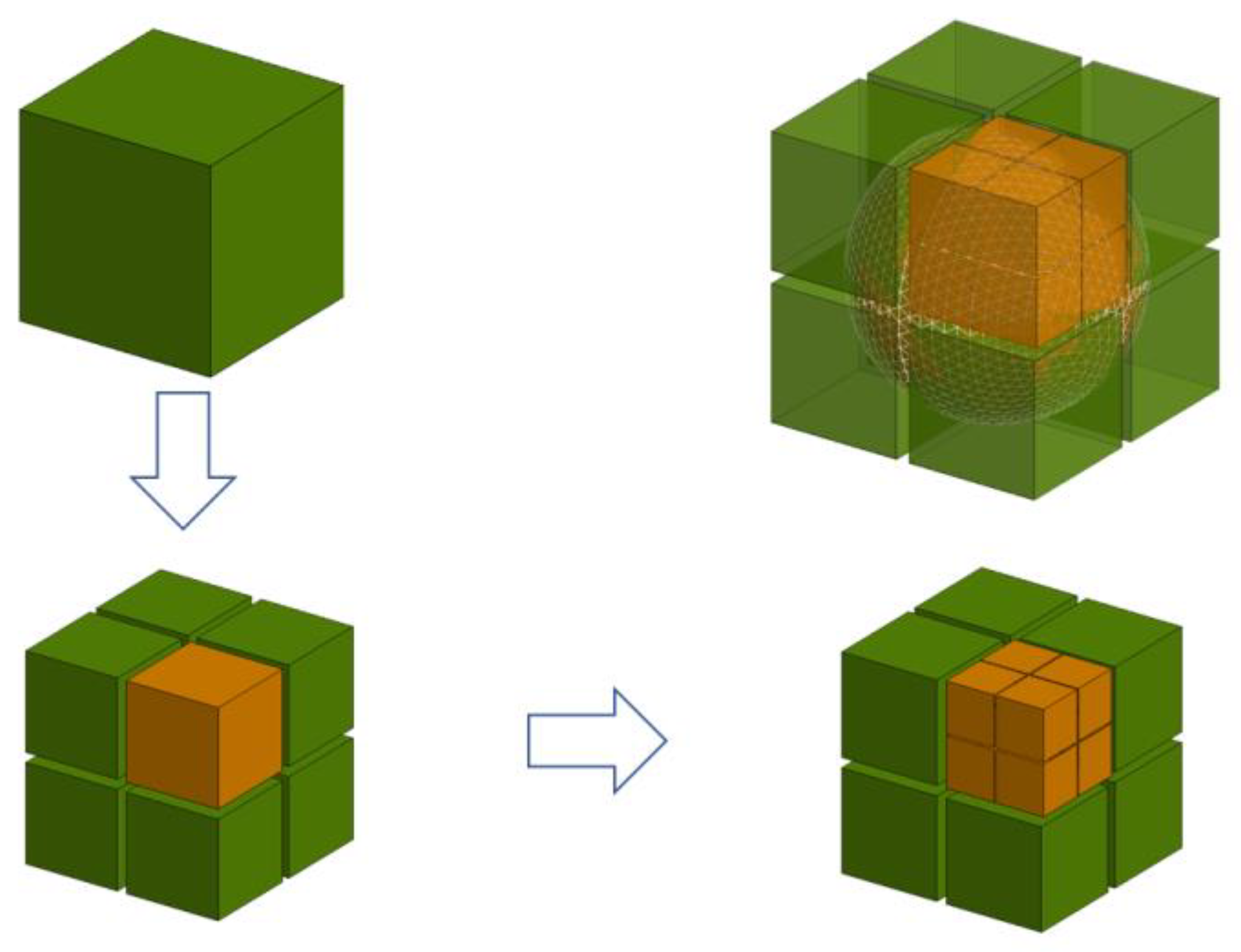
3.1. Group the Basis Function

We need to calculate the incidence and scattering angles by (9). The surface of the electrically large target is meshed by using the triangles, and then the RWG basis functions are defined on each pair of triangle elements.

In the ACA approach, we need to group the RWG basis functions on the surface of the electrically large target, as shown in Figure 3.

Firstly, the maximum values $(X_{\max },Y_{\max },Z_{\max })$ and the minimum values $(X_{\min },Y_{\min },Z_{\min })$ of all triangle vertices positions on the target surface are obtained. A cube is introduced by selecting $(X_{\min },Y_{\min },Z_{\min })$ as the vertex position and $MAX\left\{\left|X_{\max }-X_{\min }\right|,\left|Y_{\max }-Y_{\min }\right|,\left|Z_{\max }-Z_{\min }\right|\right\}$ as the edge length, where $X_{\max }$, $X_{\min }$, $Y_{\max }$, $Y_{\min }$, $Z_{\max }$ and $Z_{\min }$ denote the maximum and minimum values of the $X$-axis, $Y$-axis and $Z$-axis components of the triangle’s vertex coordinates, respectively. $MAX\{·\}$ is the maximum value and $|·|$ represents the absolute value. The cube is divided into eight cube blocks of equal size. Then, the RWG basis functions in the same cube block are classified as a group. Each small cube block is then divided into eight smaller, equal-sized cube blocks by using the octree structure. This process is repeated until the side length of the cube is less than 0.5${\lambda }_b$. Finally, we can derive the partitioned groups of RWG basis functions. Then, by using a threshold ${\lambda }_a$, the impedance matrix can be divided into two parts, which are near-field blocks and far-field blocks.

3.2. Determine Chebyshev–Gauss Frequency Sampling Points

The Chebyshev–Gauss frequency points ${\tilde{k}}_i$ are calculated by:

$${\tilde{k}}_i=\cos \left[\frac{i-0.5}{g}\pi \right]\hspace{1em}i=1,2,3\cdots g$$

(10)

where $g$ denotes the truncated order of the Chebyshev series.

The Chebyshev–Gauss sampling points $k_i$ are obtained by transforming the ${\tilde{k}}_i$ from the interval $\left[-1,1\right]$ to the desired band $\left[k_a,k_b\right]$ by:

$$k_i=\frac{{\tilde{k}}_i\left(k_b-k_a\right)+\left(k_a+k_b\right)}{2}$$

(11)

where $k_i$ denotes the i-th Chebyshev–Gauss frequency sampling point over the desired frequency band. $k_a$ and $k_b$ correspond to the wave numbers at the start and cut-off frequency, respectively.

3.3. Fill Impedance Matrix

The far-field blocks are compressed into low-rank matrices by using ACA, and the near-field blocks are filled by the traditional MoM.

The far-field blocks at the sampling points are compressed into the form of the product of two low-rank matrices by ACA, which can be expressed as:

$$Z_{far}^y(k_i)=U_{{}_{y,k_i}}^{C_{{}_{y,k_i}}}{V}_{y,k_i}^{C_{{}_{y,k_i}}}\hspace{1em}y=1,2,3\cdots \sigma$$

(12)

where $Z_{far}^y(k_i)$ denotes the y-th far-field block at the i-th Chebyshev–Gauss frequency sampling point $k_i$, and $\sigma$ is the total number of far-field blocks. $U_{y,k_i}^{C_{{}_{y,k_i}}}$ and $V_{y,k_i}^{C_{{}_{y,k_i}}}$ represent the low-rank column matrix and low-rank row matrix, respectively. $C_{{}_{y,k_i}}$ denotes the rank of the low rank matrix after compressive decomposition.

The rank $C_{{}_{y,k_i}}$ of the compressed low-rank matrix is obtained by:

$$\Vert R^{y,k_i}\Vert =\Vert {\overline{Z}}_{far}^y(k_i)-Z_{far}^y(k_i)\Vert \le \epsilon \Vert Z_{far}^y(k_i)\Vert$$

(13)

where $\mathsf{\epsilon }$ denotes the error iteration threshold, $R^{y,k_i}$ is the error matrix, $\Vert ·\Vert$ represents the Frobenious norm of the matrix and ${\overline{Z}}^y{}_{far}(k_i)$ denotes the exact value of the y-th far-field block.

The implementation process of the ACA algorithm at the i-th Chebyshev–Gauss frequency sampling point $k_i$ can be divided into the initialization part and the k-th iteration.

3.3.1. Initialization Section

(1)

Initialize the line index $I_1=1$, and initialize ${\tilde{Z}}_{far}^{y,k_i}=0$.

(2)

Initialize the $I_1$ row of the error matrix: $R^{y,k_i}\left(I_1,:\right)=Z_{{}_{far}}^{y,k}\left(I_1,:\right)$.

(3)

Find the index in the first column so that $J_1$: $\left|R^{y,k_i}\left(I_1,J_1\right)\right|={\max }_j\left|R^{y,k_i}\left(I_1,j\right)\right|$.

(4)

$v_1^{y,k_i}=R^{y,k_i}\left(I_1,:\right)/R^{y,k_i}\left(I_1,J_1\right)$.

(5)

Initialize the first column of the error matrix $R^{y,k_i}\left(:,J_1\right)=Z_{{}_{far}}^{y,k}\left(:,J_1\right)$.

(6)

Obtain the first column of the U matrix $u_1^{y,k}=R^{y,k_i}\left(:,J_1\right)$.

(7)

Calculate the approximation matrix ${\Vert {\tilde{Z}}_{y,k_i}^{\left(1\right)}\Vert }^2={\Vert {\tilde{Z}}_{y,k_i}^{\left(0\right)}\Vert }^2+{\Vert u_1^{y,k_i}\Vert }^2{\Vert v_1^{y,k_i}\Vert }^2$.

(8)

Determine the index of the second row $I_2$: $\left|R^{y,k_i}\left(I_2,J_1\right)\right|={\max }_i\left|R^{y,k_i}\left(i,J_1\right)\right|,i\ne I_1$.

3.3.2. k-th Iteration

(1)

Update the ($I_k$)-th row of the approximate error matrix: $\left|R^{y,k_i}\left(I_k,:\right)\right|=Z_{{}_{far}}^{y,k_i}\left(I_k,:\right)-{\displaystyle \sum _{l=1}^{k-1}{\left(u_l^{y,k_i}\right)}_{I_k}{v}_l^{y,k_i}}$.

(2)

Find the maximum value in the ($I_k$)-th row to determine the $J_k$ column $J_k$: $\left|R^{y,k_i}\left(I_k,J_k\right)\right|={\max }_j\left|R^{y,k_i}\left(I_k,j\right)\right|,j\ne J_1,J_2,\cdots ,J_k$.

(3)

The k-th row of the V matrix is obtained $v_k^{y,k_i}=R^{y,k_i}\left(I_k,:\right)/R^{y,k_i}\left(I_k,J_k\right)$.

(4)

Update the ($J_k$)-th column of the approximate error matrix: $\left|R^{y,k_i}\left(:,J_k\right)\right|=Z_{far}^{y,k_i}\left(:,J_k\right)-{\displaystyle \sum _{l=1}^{k-1}{\left(v_l^{y,k_i}{}_l\right)}_{J_k}{u}_l^{y,k_i}}$.

(5)

The k-th column of the U matrix is obtained $u_k{}^{y,k_i}=R^{y,k_i}\left(:,J_k\right)$.

(6)

${\Vert {\tilde{Z}}_{y,k_i}^{\left(k\right)}\Vert }^2={\Vert {\tilde{Z}}_{y,k_i}^{\left(k-1\right)}\Vert }^2+2{\displaystyle \sum _{j=1}^{k-1}\left|{(u_j^{y,k_i})}^T{u}_k^{y,k}\right|\left|{(v_j^{y,k_i})}^T{v}_k{}^{y,k_i}\right|+{\Vert u_k^{y,k}\Vert }^2{\Vert v_k^{y,k}\Vert }^2}$.

(7)

If $\Vert u_k^{y,k}\Vert \Vert v_k^{y,k}\Vert \le \epsilon \Vert {({\tilde{Z}}_{far}^{y,k_i})}^{(k)}\Vert$, then the iteration is terminated; otherwise, continue to the next step.

(8)

Find the next row index $I_{k+1}$: $\left|R^{y,k_i}\left(I_{k+1},J_k\right)\right|={\max }_i\left|R^{y,k_i}\left(i,J_k\right)\right|,i\ne I_1,I_2,\cdots ,I_k$.

• where the termination condition of (7) is based on the selection condition of rank $r$ by $\Vert R_{y,k_i}^{m\times n}\Vert =\Vert Z_{y,k_i}^{m\times n}-{\tilde{Z}}_{y,k_i}^{m\times n}\Vert \approx \Vert u_k{}^{y,k_i}\Vert \Vert v_k^{y,k_i}\Vert$.

3.4. Solve Wideband Surface Currents

By using MoM, the matrix equation over a broad frequency band can be given by:

$$Z(k_i)I(k_i)=W(k_i)$$

(14)

where $Z(k_i)$ denotes the impedance matrix at the i-th Chebyshev sampling point $k_i$ and it can be divided into $o$ near-field blocks and $\sigma$ far-field blocks. $I(k_i)$ represents the surface currents at the i-th Chebyshev–Gauss frequency sampling point $k_i$, and $W(k_i)$ represents the excitation vector. The surface currents of near-field blocks at each Chebyshev sampling point can be obtained by (14).

The product of two low-rank matrices $U_{y,k_i}^{C_{{}_{y,k_i}}}$ and $V_{y,k_i}^{C_{{}_{y,k_i}}}$ is used to represent the far-field blocks. The matrix Equation (14) can be rewritten as:

$$Z_{far}^y(k_i)I_{far}^{y,k_i}(k_i)=U_{y,k_i}^{C_{y,k_i}}(V_{y,k}^{C_{y,k_i}}{I}_{far}^{y,k_i}(k_i))$$

(15)

where $I_{far}^{y,k_i}(k_i)$ denotes the current coefficient corresponding to the y-th far-zone block at $k_i$ of the i-th Chebyshev–Gauss frequency sampling point.

Then, the electric currents $I(k_i)$ can be calculated by:

$$I\left(k_i\right)=I\left(\frac{{\tilde{k}}_i\left(k_b-k_a\right)+\left(k_b+k_a\right)}{2}\right)$$

(16)

and the Chebyshev approximation for $I\left(k_i\right)$ is given by:

$$I\left(k_i\right)=I\left(\frac{{\tilde{k}}_i\left(k_b-k_a\right)+\left(k_b+k_a\right)}{2}\right)\simeq {\displaystyle \sum _{\gamma =0}^{g-1}{c}_{\gamma }{T}_{\gamma }\left({\tilde{k}}_i\right)}-\frac{c_0}{2}$$

(17)

$$c_{\gamma }=\frac{2}{g}{\displaystyle \sum _{i=0}^{g}I\left(k_i\right)T_{\gamma }\left({\tilde{k}}_i\right)}$$

(18)

where $\gamma$ represents the order of Chebyshev polynomial, $\gamma =1,2,3\cdots g$. The stated Chebyshev polynomial $T_{\gamma }({\tilde{k}}_i)$ is determined by:

$$\{\begin{array}{l}{T}_0({\tilde{k}}_i)=1\\ T_1({\tilde{k}}_i)={\tilde{k}}_i\\ T_{\gamma +1}({\tilde{k}}_i)=2{\tilde{k}}_i{T}_{\gamma }({\tilde{k}}_i)-T_{\gamma -1}({\tilde{k}}_i)(g\ge \gamma \ge 2)\end{array}$$

(19)

Finally, to obtain a wider frequency band, the Chebyshev series is replaced by a rational function named Maehly approximation:

$$I\left(k_i\right)\simeq R_{LM}\left({\tilde{k}}_i\right)=\frac{P_L\left({\tilde{k}}_i\right)}{Q_M\left({\tilde{k}}_i\right)}=\frac{a_0{T}_0\left({\tilde{k}}_i\right)+a_1{T}_1\left({\tilde{k}}_i\right)+\cdots a_L{T}_L\left({\tilde{k}}_i\right)}{b_0{T}_0\left({\tilde{k}}_i\right)+b_1{T}_1\left({\tilde{k}}_i\right)+\cdots b_M{T}_M\left({\tilde{k}}_i\right)}$$

(20)

where $b_0$ is set to be 1, as the rational function can be divided by an arbitrary constant. $\mathrm{g}=L+2M$, where $L$ and $M$ are the Chebyshev polynomial expansion orders of $P_L\left({\tilde{k}}_i\right)$ and $Q_M\left({\tilde{k}}_i\right)$, respectively.

The unknown coefficients $a_i\left(i=0,1,\dots ,L\right)$ and $b_i\left(i=0,1,\dots ,M\right)$ can be solved by:

$$\{\begin{array}{l}{a}_0=\frac{1}{2}{b}_0{c}_0+\frac{1}{2}{\displaystyle \sum _{j=1}^M{b}_j{c}_j}\\ a_i=c_i+\frac{1}{4}{b}_i{c}_0+\frac{1}{2}{\displaystyle {\sum }_{j=1}^M{b}_j\left(c_{j+i}+c_{\left|j-i\right|}\right)}\hspace{1em}\hspace{1em}i=1,2,\dots ,L\end{array}$$

(21)

$${\displaystyle \sum _{j=1}^M{b}_j\left(c_{L+i+j}+c_{L+i-j}\right)}=-2c_{L+i},\hspace{1em}i=1,2,\dots ,M$$

(22)

A pseudocode is shown in Algorithm 1 to help readers better understand the procedure of the hybrid ACA-CAT algorithm.

Algorithm 1 the hybrid ACA-CAT algorithm

Input:  $({\theta }_{inc},{\phi }_{inc})$,$({\theta }_{sca},{\phi }_{sca})$,$\left[k_a,k_b\right]$, the Chebyshev polynomial expansion orders L.

Output: the coefficients of Chebyshev series, the Maehly approximation coefficients, $a_i,b_i$

1: Group of RWG basis functions on the target surface

2: Dividing the impedance matrix into near-field and far-field blocks

3:  for $k_i=1$ to $g$ do

4:    Calculate the impedance matrix near-field block $Z_{near}^y\left(k_i\right)$

5:    Compress the far-field blocks $Z_{far}^y\left(k_i\right)$ at the sampling points into the form of the product of two low-rank matrices by ACA: $Z_{far}^y(k_i)=U_{{}_{y,k_i}}^{C_{{}_{y,k_i}}}{V}_{y,k_i}^{C_{{}_{y,k_i}}}$

6:    Then solve $Z(k_i)I(k_i)=W(k_i)$

7:    Compute the Coefficients of Chebyshev series and the Maehly approximation coefficients, $a_i,b_i$

8:  end for

9:  for $\rho =1$ to frenum do

10: Calculate the surface current at the wave number corresponding to each frequency point in the broadband: $I(k_{\rho })={\displaystyle \sum _{\gamma =0}^{g-1}(\frac{2}{g}{\displaystyle \sum _{j=1}^{g}I\left(k_j\right)T_{\gamma }({\tilde{k}}_j)}{T}_{\gamma }({\tilde{k}}_{\rho })})-\frac{1}{g}{\displaystyle \sum _{j=1}^{g}I\left(k_j\right)}$

11: Obtain the radar scattering cross section at the wave number corresponding to each frequency point in the broadband of the target: $\sigma (k_{\rho })=\underset{R\to \infty }{\lim }4\pi R^2\frac{{\left|j{k}_{\rho }{Z}_0{\widehat{r}}^{\prime }\times {\widehat{r}}^{\prime }\times {\displaystyle {\iint }_S\left[{\displaystyle \sum _{d=1}^N{I}_d\left(k_{\rho }\right)f_d\left(r_d\right)}\right]\frac{e^{-j{k}_{\rho }R}}{4\pi R}d{r}_d}\right|}^2}{{\left|E_{in}\right|}^2}$

12:  end for

4. Numerical Simulation Results and Analysis

In order to validate the accuracy and efficiency of the hybrid ACA-CAT method, we present three numerical examples. The geodetic coordinates of the targets are all (0, 0, 10,000), and the pitch, yaw and roll angles of the targets are all 0°, 0° and 20°. The MoM iterative solver and the iterative solver for ACA and ACA-CAT all adopt the biconjugate gradient stabilization method. The tolerance of the iterative solver for ACA and ACA-CAT is 0.001. All simulations have been implemented using an Intel Core i5-8th CPU with 16 GB of RAM, and the metric root mean square error (RMSE) is employed as:

$$\mathrm{RMSE}=\sqrt{\frac{{\displaystyle \sum _{i=1}^n{(RCS-RC{S}^{\prime })}^2}}{N_{fre}}}$$

(23)

where RCS indicates the value calculated by conventional MoM or ACA, and $RC{S}^{\prime }$ indicates the value calculated by ACA-CAT. $N_{fre}$ stands for the number of frequency points.

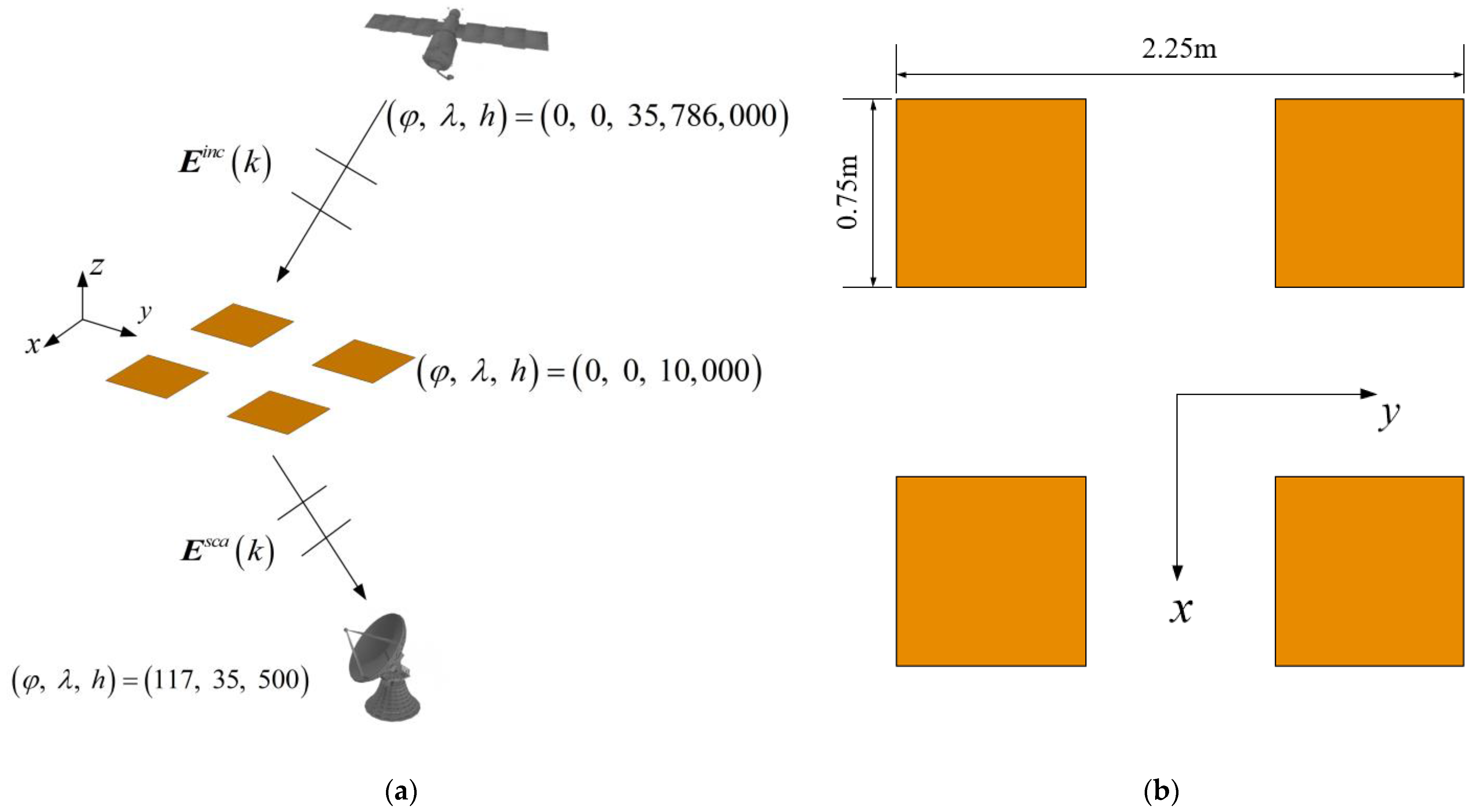
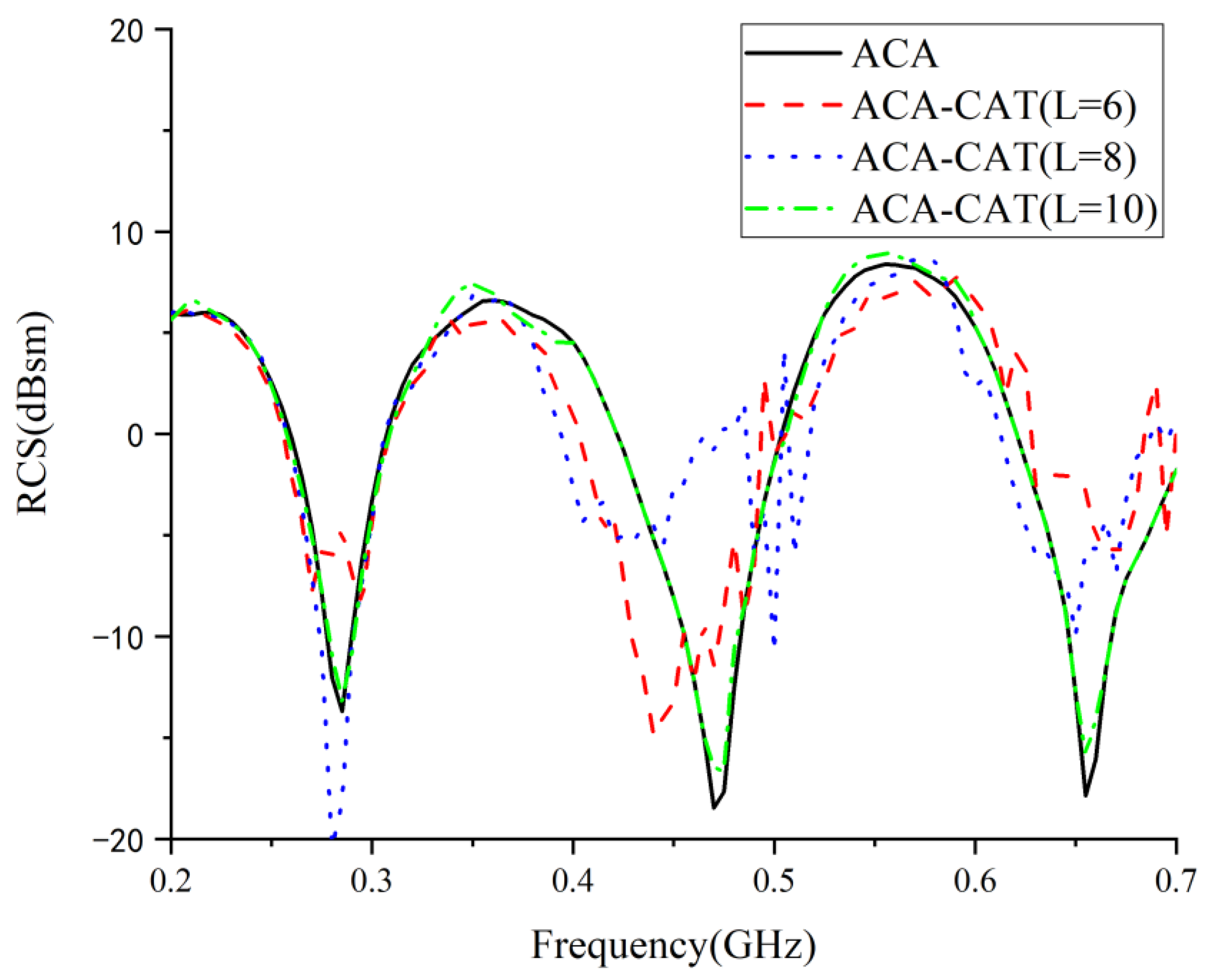
4.1. A Four Patch Array

The first example we consider is a PEC patch array, as illustrated in Figure 4a. Each patch element has a size of 75 cm $\times$ 75 cm, and the size of the model is shown in Figure 4b. Each patch element is discretized into 440 triangular elements, resulting in 2528 unknowns. The geodetic coordinates of the satellite and PBR are (0, 0, 35,786,000) and (117, 35, 500), respectively. The incident angle is (θ_inc, φ_inc) = (20°, 270°), and the scattering angle is (θ_sca, φ_sca) = (137°, 39°), which can be calculated by Equation (9). The working frequency band is 0.2 to 0.7 GHz and the step frequency is 5 MHz.

Figure 5 illustrates the θθ polarized BCS of the patch array over the 0.2–0.7 GHz frequency band for three different ACA-CAT orders (L = 4, 6, 8). The point-by-point ACA simulations are compared. It can be seen that as we increase the order of ACA-CAT, we will achieve a better result. The MoM, ACA, ACA-CAT and MoM-AWE numerical results are shown in Figure 6, and the results obtained by ACA-CAT agree well with those obtained by MoM and ACA.

To further validate the correctness of the proposed ACA-CAT algorithm for this example, the ACA-CAT method was used to compute the bistatic RCS at the non-Gaussian sampling point and to compare it with MoM. Figure 7 shows the θθ polarized bistatic results for the plane wave incidence directions of θ_inc = 4° and φ_inc = 0° and bistatic acceptance angles of θ_sca = $0\sim {180}^{\circ }$ and φ_sca = 0° at 0.35 GHz calculated by the ACA-CAT method at L = 8. Adequate agreement can be observed.

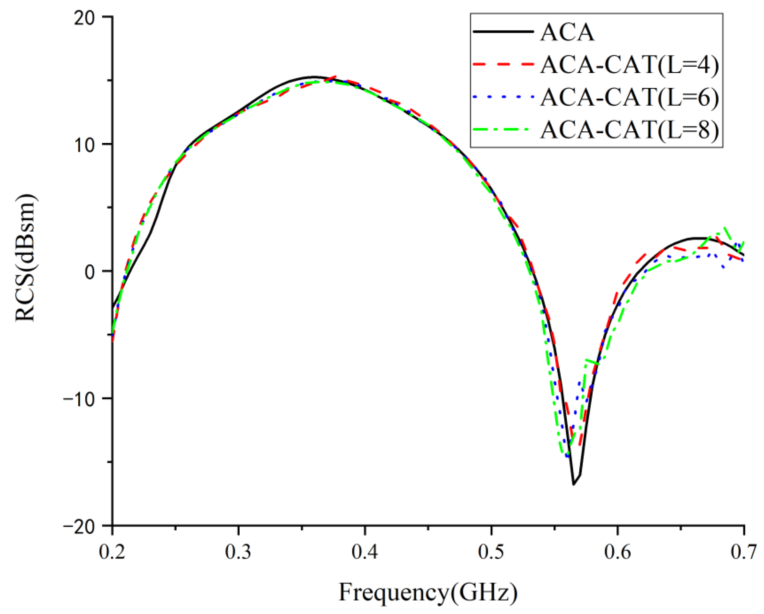
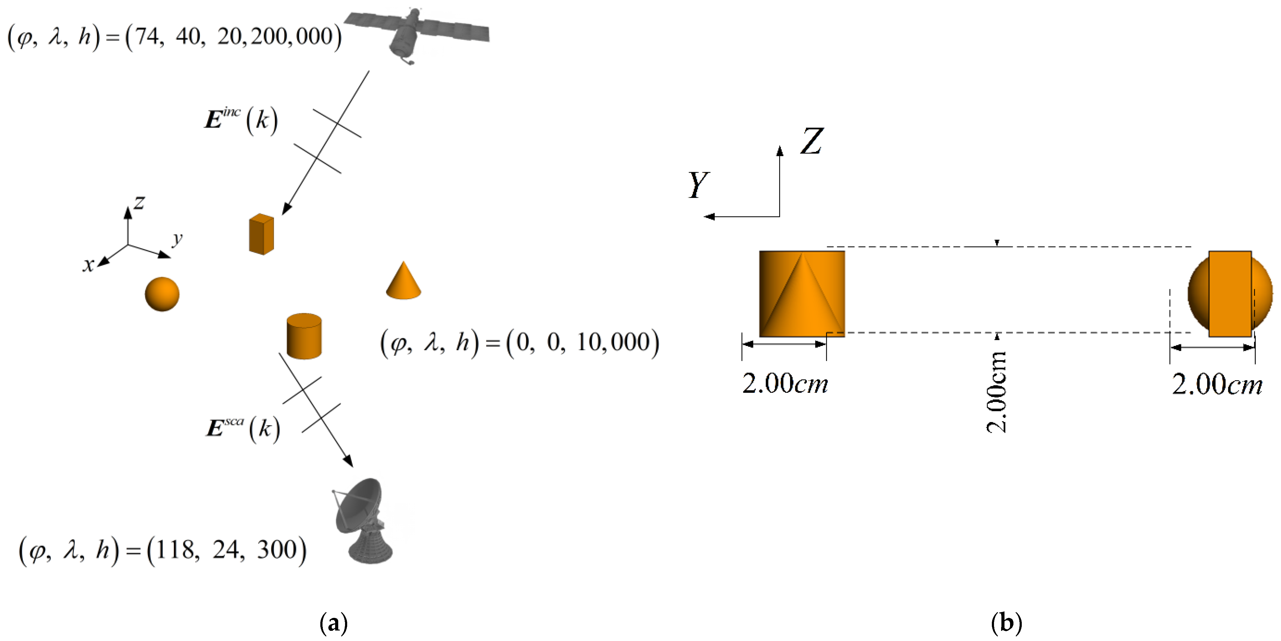
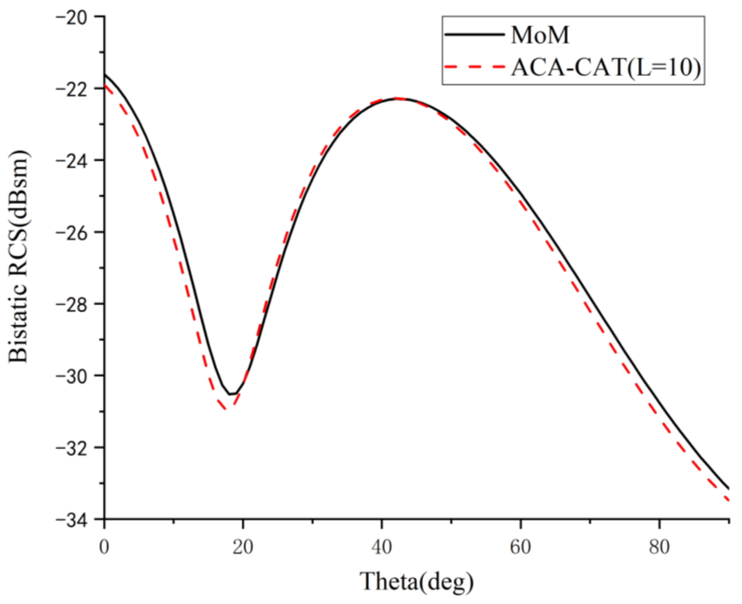
4.2. Four Discrete Objects

Our second example is four discrete objects consisting of a rectangular, a cylinder, a sphere and a cone, as shown in Figure 8a; the details of the model are shown in Figure 8b. The four discrete objects are discretized into 1318 triangular elements, resulting in 1977 unknowns. The geodetic coordinates of the satellite and PBR are (74, 40, 20,200,000) and (118, 24, 300). The incident angle is (θ_inc, φ_inc) = (30°, 180°), and the scattering angle is (θ_sca, φ_sca) = (101°, 42°), which can be calculated by Equation (9). The working frequency band is 2 to 12 GHz and the step frequency is 100 MHz.

Figure 9 illustrates the θθ polarized BCS of the four discrete objects in the 2–12 GHz range for three different ACA-CAT orders (L = 2, 4, 6). ACA-CAT was compared with point-by-point ACA. With the increase in the order of CAT, we achieve a better result. The MoM, ACA, ACA-CAT and MoM-AWE results are shown in Figure 10. The results obtained by ACA-CAT are consistent with those obtained by MoM and ACA.

In order to further verify the correctness of the proposed ACA-CAT algorithm, the ACA-CAT method is used to calculate the bistatic RCS of non-Gaussian sampling points, and is compared with MoM. Figure 11 shows the θθ polarized bistatic results for the plane wave incidence directions of θ_inc = 0° and φ_inc = 0° and bistatic acceptance angles of θ_sca = $0\sim {90}^{\circ }$ and φ_sca = 0° at 4 GHz calculated using the ACA-CAT method at L = 8. The BCS result is compared with the BCS result calculated by the method of moments, which has adequate consistency and verifies the accuracy of the algorithm.

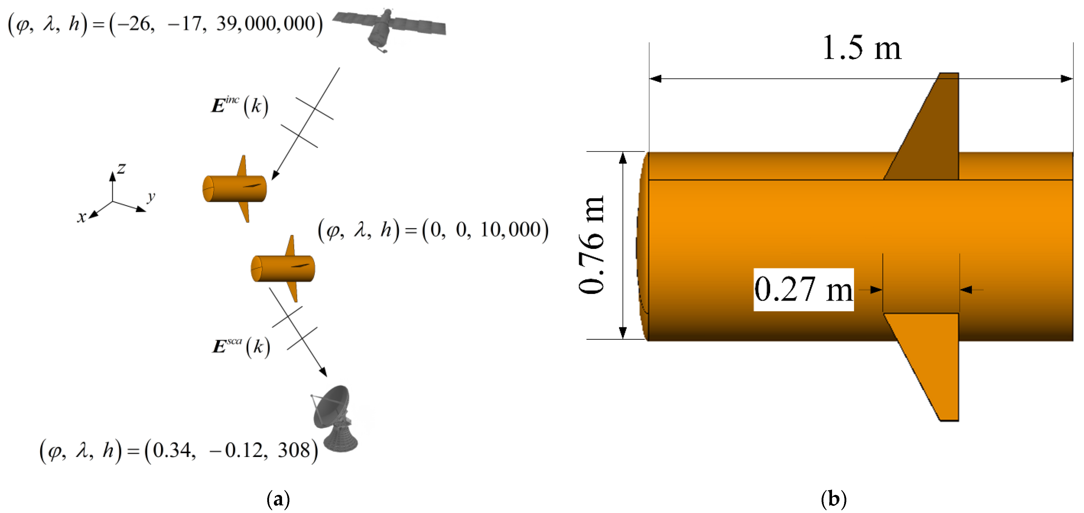
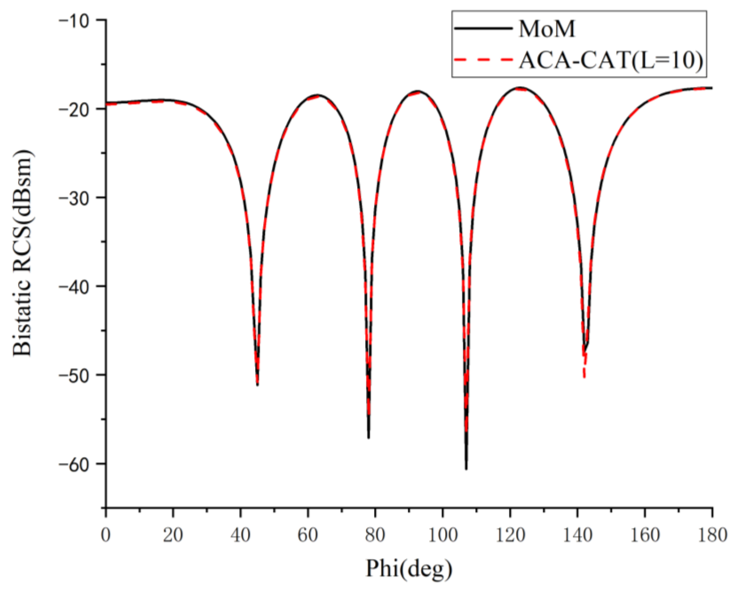
4.3. A Missile Model

Our third example is a simple dual missile. Both missiles are the same size, as shown in Figure 12a, and the details of the model are shown in Figure 12b. The spacing between missiles is 3.6 m. The dual missile can be discretized into 7844 elements so that the number of unknowns is 11,738. Satellite and radar geodetic coordinates are (−26, −17, 39,000,000) and (0.34, −0.12, 308). The incident angle is (θ_inc, φ_inc) = (30°, 180°), and the scattering angle is (θ_sca, φ_sca) = (90°, 20°), which can be calculated by Equation (9). The working frequency band is 0.2 to 0.7 GHz. The step frequency is 5 MHz.

Figure 13 illustrates the θθ polarized BCS of the dual missile in the 2–7 GHz range for three different ACA-CAT orders (L = 6, 8, 10). A comparison between ACA-CAT and point-by-point ACA is made. It can be seen that the numerical results of ACA-CAT improve with the increase in order L. The MoM, ACA, ACA-CAT and MoM-AWE results are shown in Figure 14. The results obtained by ACA-CAT are consistent with those obtained by MoM and ACA.

In order to further verify the accuracy of the proposed ACA-CAT algorithm in the example, the ACA-CAT method was used to calculate the bistatic RCS of non-Gaussian sampling points and compared with MoM. Figure 15 shows the θθ polarized bistatic results for the plane wave incidence directions of θ_inc = 30° and φ_inc = 180° and bistatic acceptance angles of θ_sca = 20° and φ_sca = $0\sim {180}^{\circ }$ at 0.5 GHz non-Gaussian sampling points calculated using the ACA-CAT method at L = 10. The BCS result is compared with the BCS result calculated by the moment method. The two results agree well, which verifies the accuracy of the algorithm.

Table 1. CPU time, memory requirements and RMSE of ACA-CAT for wideband RCS simulation of three examples at different orders.

Examples	Methods	Memory (MB)	CPU Time (s)	RMSE (dBsm)
patch array	ACA-CAT_L = 4 ACA-CAT_L = 6 ACA-CAT_L = 8 ACA	37.5 37.5 37.5 37.5	329 495 683 5780	1.30 1.23 0.84 /
discrete objects	ACA-CAT_L = 2 ACA-CAT_L = 4 ACA-CAT_L = 6 ACA	49.9 45.9 45.9 49.6	180 420 826 5385	1.28 0.70 0.61 /
missile model	ACA-CAT_L = 6 ACA-CAT_L = 8 ACA-CAT_L = 10 ACA	530.3 530.3 530.3 530.3	68,207 90,942 113,678 378,927	4.91 3.08 0.95 /

shows the comparison of the memory requirements, total CPU time and RMSE of the ACA-CAT technique at three different orders for the patch array, the four discrete objects and the missile model. It can be observed that as we increased the order of the ACA-CAT, the CPU time gradually increased. The reason for this is that the higher the order chosen, the more currents that need to be calculated and stored at the Chebyshev–Gauss sampling frequency points.

The comparison of the memory requirement, CPU time and RMSE of four different algorithms is illustrated in

Table 2. CPU time, memory requirements and RMSE of four different methods for wideband RCS simulation of three examples.

Examples	Methods	Memory (MB)	CPU Time (s)	RMSE (dBsm)
patch array	MoM ACA ACA-CAT_L = 8 MoM-AWE_Q = 8	97.5 37.5 37.5 780.1	11,479 5460 629	/ 0.24 1.34
			2726	0.17
discrete objects	MoM ACA ACA-CAT_L = 6 MoM-AWE_Q = 8	59.6 45.3 48.7 477.1	8680 5090 826 1652	/ 0.09 0.72 0.11
missile model	MoM ACA ACA-CAT_L = 10 MoM-AWE_Q = 8	2112.4 530.3 530.3	589,831 378,927 113,678	/ 0.25 1.15
		16,899.2	164,404	0.41

. It can be seen that compared to ACA, the ACA-CAT can reduce CPU time by 88.18%, 84.66% and 70.02% for the patch array, the four discrete objects and the missile model, respectively. Note that compared with the MoM, the memory requirement of ACA-CAT can achieve 61.54%, 23.99% and 74.90% reduction for the patch array, the four discrete objects and the missile model, respectively. Even compared to the MoM-AWE, the memory requirement of ACA-CAT can achieve 95.19%, 89.80% and 96.86% reduction for the patch array, the four discrete objects and the missile model, respectively.

5. Conclusions

The hybrid ACA-CAT is proposed to solve the wideband electromagnetic bistatic scattering problem of 3D PEC targets based on a non-cooperative satellite-borne illuminator. The ACA technique can be employed to reduce the memory requirement and computation time by compressing the low-rank matrix blocks. By introducing the idea of CAT, only the currents at Chebyshev nodes are calculated to alleviate the problems of massive calculation and time consumption. Finally, the numerical results show that the ACA-CAT solution can significantly reduce the CPU time with a slight loss of precision. Although only the BCS based on the satellite source is presented, the proposed algorithm can be employed to calculate the BCS based on some other non-cooperative sources, such as base station signals, broadcast signals and mobile communication signals. Since the wideband currents of the targets are obtained, the hybrid ACA-CAT method can be used to not only compute the monostatic RCS of the targets over a broad frequency band, but also calculate the BCS of the objects at any scattering angle and any frequency point.

References

1. Zhao, Z.; Zhou, X.; Zhu, S.; Hong, S. Reduced Complexity Multipath Clutter Rejection Approach for DRM-Based HF Passive Bistatic Radar. IEEE Access 2017, 61, 20228–20234. [Google Scholar] [CrossRef]
2. Palmer, J.E.; Harm, H.A.; Searle, S.J.; Davis, L. DVB-T Passive Radar Signal Processing. IEEE Trans. Signal Process. 2013, 61, 2116–2126. [Google Scholar] [CrossRef]
3. Qiu, W.; Giusti, E.; Bacci, A.; Martorella, M.; Zhao, H.Z.; Fu, Q. Compressive sensing-based algorithm for passive bistatic ISAR with DVB-T signals. IEEE Trans. Aerosp. Electron. Syst. 2015, 51, 2166–2180. [Google Scholar] [CrossRef]
4. Navrátil, V.; Garry, J.L.; O’Brien, A.; Smith, G.E. Utilization of terrestrial navigation signals for passive radar. In Proceedings of the IEEE Radar Conference, Seattle, WA, USA, 8–12 May 2017; pp. 825–829. [Google Scholar]
5. Tao, S.; Ran, T.; Yue, W.; Siyong, Z. Study of detection performance of passive bistatic radars based on FM broadcast. J. Syst. Eng. Electron. 2007, 18, 22–26. [Google Scholar] [CrossRef]
6. Shi, C.; Wang, F.; Sellathura, M.; Zhou, J. Transmitter Subset Selection in FM-Based Passive Radar Networks for Joint Target Parameter Estimation. IEEE Trans. Aerosp. Electron. Syst. 2016, 16, 6043–6052. [Google Scholar] [CrossRef]
7. Griffiths, H.D.; Long, N.R. Television based bistatic radar. IEE Proc. F Commun. Radar Signal Process. 1986, 133, 649–657. [Google Scholar] [CrossRef]
8. Tan, D.K.P.; Sun, H.; Lu, Y.; Lesturgie, M.; Chan, H.L. Passive radar using global system for mobile communication signal: Theory, implementation and measurements. IEE Proc. Radar Sonar Navigat. 2005, 152, 116–123. [Google Scholar] [CrossRef]
9. Gogineni, S.; Rangaswamy, M.; Rigling, B.D.; Nehorai, A. Ambiguity function analysis for UMTS-Based passive multistatic radar. IEEE Trans. Signal Process. 2014, 62, 2945–2957. [Google Scholar] [CrossRef]
10. Griffiths, H.D.; Garnett, A.J.; Baker, C.J.; Keaveney, S. Bistatic radar using satellite-borne illuminators of opportunity. In Proceedings of the International Conference on Radar, Brighton, UK, 12–13 October 1992; pp. 276–279. [Google Scholar]
11. Li, M.Z.; Li, X.J. Detectability of maritime targets using passive radar based on satellite-borne illuminators. In Proceedings of the International Conference on Electronics Technology, Chengdu, China, 10–13 May 2019; pp. 273–276. [Google Scholar]
12. Pastina, D.; Santi, F.; Pieralice, F.; Ma, H.; Tzagkas, D.; Antoniou, M.; Cherniakov, M. Maritime moving target long time integration for GNSS-Based passive bistatic radar. IEEE Trans. Aerosp. Electron. Syst. 2018, 54, 3060–3083. [Google Scholar] [CrossRef] [Green Version]
13. Rosenberg, L.; Ouellette, J.D.; Dowgiallo, D.J. Passive bistatic sea clutter statistics from spaceborne illuminators. IEEE Trans. Aerosp. Electron. Syst. 2020, 56, 3971–3984. [Google Scholar] [CrossRef]
14. Yang, M.L.; Wu, B.Y.; Gao, H.W.; Sheng, X.Q. A Ternary Parallelization Approach of MLFMA for Solving Electromagnetic Scattering Problems With Over 10 Billion Unknowns. IEEE Trans. Antennas Propag. 2019, 67, 6965–6978. [Google Scholar] [CrossRef]
15. Hughey, S.; Aktulga, H.M.; Vikram, M.; Lu, M.; Shanker, B.; Michielssen, B. Parallel Wideband MLFMA for Analysis of Electrically Large, Nonuniform, Multiscale Structures. IEEE Trans. Antennas Propag. 2019, 67, 1094–1107. [Google Scholar] [CrossRef]
16. Khalichi Ergül, Ö.; Takrimi, M.; Ertürk, V.B. Broadband Analysis of Multiscale Electromagnetic Problems: Novel Incomplete-Leaf MLFMA for Potential Integral Equations. IEEE Trans. Antennas Propag. 2021, 69, 9032–9037. [Google Scholar] [CrossRef]
17. Wu, C.B.; Guan, L.; Gu, P.F.; Chen, R.S. Application of Parallel CM-MLFMA Method to the Analysis of Array Structures. IEEE Trans. Antennas Propag. 2021, 9, 6116–6121. [Google Scholar] [CrossRef]
18. Karaosmanoğlu, B.; Ergül, Ö. Acceleration of MLFMA Simulations Using Trimmed Tree Structures. IEEE Trans. Antennas Propag. 2021, 69, 356–365. [Google Scholar] [CrossRef]
19. Sharma, S.; Triverio, P. AIMx: An Extended Adaptive Integral Method for the Fast Electromagnetic Modeling of Complex Structures. IEEE Trans. Antennas Propag. 2021, 69, 8603–8617. [Google Scholar] [CrossRef]
20. Yang, K.; Ning, C.; Yin, W.Y. Characterization of Near-Field Coupling Effects From Complicated Three-Dimensional Structures in Rectangular Cavities Using Fast Integral Equation Method. IEEE Trans. Electromagn. Compat. 2017, 59, 639–645. [Google Scholar] [CrossRef]
21. Seo, S.W.; Lee, J.F. A fast IE-FFT algorithm for solving PEC scattering problems. IEEE Trans. Magn. 2005, 41, 1476–1479. [Google Scholar]
22. Gibson, W.C. Efficient Solution of Electromagnetic Scattering Problems Using Multilevel Adaptive Cross Approximation and LU Factorization. IEEE Trans. Antennas Propag. 2020, 68, 3815–3823. [Google Scholar] [CrossRef]
23. Zhao, K.; Vouvakis, M.N.; Lee, J.-F. Application of the multilevel adaptive cross-approximation on ground plane designs. IEEE Int. Symp. Electromagn. Compat. 2004, 1, 124–127. [Google Scholar]
24. Zhao, K.; Vouvakis, M.N.; Lee, J.-F. The Adaptive Cross Approximation Algorithm for Accelerated Method of Moments Computations of EMC problems. IEEE Trans. Electromagn. Compat. 2005, 47, 763–773. [Google Scholar] [CrossRef]
25. Wu, Q.Q.; Chen, J.Z.; Wu, Z.Q.; Gong, H.W. Synthesis and Design of 5G Duplexer Based on Optimization Method. ZTE Commun. 2022, 20, 70–76. [Google Scholar]
26. Jeong, Y.R.; Hong, I.P.; Lee, K.W.; Lee, J.H.; Yook, J.G. Fast Frequency Sweep Using Asymptotic Waveform Evaluation Technique and Thin Dielectric Sheet Approximation. IEEE Trans. Antennas Propag. 2016, 64, 1800–1806. [Google Scholar] [CrossRef]
27. Hassan, M.A.M.; Kishk, A.A. A Combined Asymptotic Waveform Evaluation and Random Auxiliary Sources Method for Wideband Solutions of General-Purpose EM Problems. IEEE Trans. Antennas Propag. 2019, 67, 4010–4021. [Google Scholar] [CrossRef]
28. Kong, W.J.; Xie, J.; Zhou, F.; Yang, X.; Wang, R.; Zheng, K. An efficient FG-FFT with optimal replacement scheme and inter/extrapolation method for analysis of electromagnetic scattering over a frequency band. IEEE Access 2019, 7, 127511–127520. [Google Scholar] [CrossRef]
29. Wang, X.; Zhang, S.; Xue, H.; Gong, S.X.; Liu, Z.L. A Chebyshev approximation technique based on AIM-PO for wide-band analysis. IEEE Antennas Wireless Propag. Lett. 2016, 15, 93–97. [Google Scholar] [CrossRef]
30. Wang, X.; Gong, H.X.; Zhang, S.; Liu, Y.; Yang, R.P.; Liu, C.H. Efficient RCS computation over a broad frequency band using subdomain MoM and Chebyshev approximation technique. IEEE Access 2020, 8, 33522–33531. [Google Scholar] [CrossRef]
31. Slone, R.D.; Lee, R.; Lee, J.F. Multipoint Galerkin asymptotic waveform evaluation for model order reduction of frequency domain FEM electromagnetic radiation problems. IEEE Trans. Antennas Propag. 2001, 49, 1504–1513. [Google Scholar] [CrossRef] [Green Version]
32. Peng, Z.; Sheng, X.Q. A bandwidth estimation approach for the asymptotic waveform technique. IEEE Trans. Antennas Propag. 2008, 56, 913–917. [Google Scholar] [CrossRef]
33. Wei, X.C.; Zhang, Y.J.; Li, E.P. The hybridization of fast multipole method with asymptotic waveform evaluation for the fast monostatic RCS computation. IEEE Trans. Antennas Propag. 2004, 52, 605–607. [Google Scholar] [CrossRef]
34. Jo, K.; Lee, M.; Sunwoo, M. Fast GPS-DR senor fusion framework: Removing the geodetic coordinate conversion process. IEEE Trans. Intell. Transp. Syst. 2016, 17, 2008–2013. [Google Scholar] [CrossRef]
Figure 1. Illustration of the passive bistatic radar system based on a non-cooperative satellite-borne illuminator.
Electronics 12 00295 g001
Figure 2. Illustration of the coordinates’ conversion from the local coordinate system to the ECEF coordinates.
Electronics 12 00295 g002
Figure 3. Schematic diagram of octree structure.
Electronics 12 00295 g003
Figure 4. Illustration of the passive bistatic radar system based on a non-cooperative satellite-borne illuminator. (a) Geometry of the patch array. (b) The model size of the patch array.
Electronics 12 00295 g004
Figure 5. Broadband BCS of a four-patch array computed by ACA-CAT for three different orders.
Electronics 12 00295 g005
Figure 6. RCS with frequency for a four-patch array by four different methods.
Electronics 12 00295 g006
Figure 7. Bistatic RCS for a four-patch array model using MoM and ACA-CAT of the non-Gaussian sampling points.
Electronics 12 00295 g007
Figure 8. Illustration of the passive bistatic radar system based on non-cooperative satellite-borne illuminator. (a) Geometry of the discrete objects. (b) The model size of the discrete objects.
Electronics 12 00295 g008
Figure 9. Broadband BCS of the four discrete objects is computed by ACA-CAT for three different orders.
Electronics 12 00295 g009
Figure 10. RCS with frequency for the four discrete objects by four different methods.
Electronics 12 00295 g010
Figure 11. Bistatic RCS for the discrete objects model using MoM and ACA-CAT of the non-Gaussian sampling points.
Electronics 12 00295 g011
Figure 12. Illustration of the passive bistatic radar system based on non-cooperative satellite-borne illuminator. (a) Geometry of the dual missile. (b) The model size of the dual missile.
Electronics 12 00295 g012
Figure 13. Broadband BCS of the dual missile is computed by ACA-CAT for three different orders.
Electronics 12 00295 g013
Figure 14. RCS with frequency for the dual missile by four different methods.
Electronics 12 00295 g014
Figure 15. Bistatic RCS for the dual missile model using MoM and ACA-CAT of the non-Gaussian sampling points.
Electronics 12 00295 g015