Improved Ship Detection with YOLOv8 Enhanced with MobileViT and GSConv

School of Automation, Jiangsu University of Science and Technology, Zhenjiang 212003, China
*
Author to whom correspondence should be addressed.
Electronics 2023, 12(22), 4666; https://doi.org/10.3390/electronics12224666
Submission received: 13 October 2023
/
Revised: 3 November 2023
/
Accepted: 13 November 2023
/
Published: 16 November 2023
Abstract
:In tasks that require ship detection and recognition, the irregular shapes of ships and complex backgrounds pose significant challenges. This paper presents an advanced extension of the YOLOv8 model to address these challenges. A lightweight visual transformer, MobileViTSF, is proposed and combined with the YOLOv8 model. To address the loss of semantic information that arises from inconsistent scales in the detection of small ships, a layer intended for the detection of small targets is introduced to lead to improved fusion of deep and shallow features. Furthermore, the traditional convolution (Conv) blocks are replaced with GSConv blocks, and a novel GSC2f block is designed for fewer model parameters and improved detection performance. Experiments on a benchmark dataset suggest that this new model can achieve significantly improved accuracy for ship detection with fewer model parameters and a reduced model size. A comparison with several other state-of-the-art methods shows that higher accuracy can be obtained for ship detection with this model. Moreover, this new model is suitable for edge computing devices, demonstrating practical application value.
1. Introduction
Ship target detection is beneficial for port management and maritime safety and has been extensively used in both the civil and military sectors. In the civilian sector, ship detection can be used for real-time monitoring of maritime traffic and also plays an important role in combating illegal fishing, pollution and smuggling. Meanwhile, in the military field, ship target detection can be used to determine whether a ship has crossed the border or not and recognize other abnormal behaviors by detecting the ship’s position, size and other information [1]. Currently, modern ships make extensive use of a wide range of sensors, including LIDAR (light detection and ranging), GPS (global positioning systems) and AIS (automatic identification systems). Through sensor fusion technology, they combine sensor data from different sources to accurately detect surrounding obstacles. However, with the development of inland transport modes and the increase in inland traffic density, traditional AISs for ships are facing challenges [2,3]. For example, although AIS can provide detailed information about nearby vessels, small boats without transmitters, buoys, etc., cannot be detected using AIS systems. In this case, it is more effective to use VTS (vessel traffic service) systems installed at coastal observatories or other key locations. VTS uses optical cameras to capture high-resolution images and video, allowing observers to remotely monitor vessel traffic in shipping lanes, ports, anchorages and critical sea areas. By monitoring and planning vessel movements in and out of busy waters, it reduces congestion and the risk of accidents and improves the safety and efficiency of shipping.
Ship target detection using computer vision is characterized by strong targeting, large detection area and excellent performance in real-time applications. Currently, research on deep learning-based ship detection algorithms has made progress. Lee et al. [4] addressed the real-time detection problem of surface USVs (unmanned surface vehicle) and experimented on a self-constructed dataset with a proposed CNN (convolutional neural network) model; the proposed model was able to process 30 frames for detection in one second. Shao et al. [5] proposed a saliency-aware ship detection framework for images obtained with a network of surveillance cameras. The missed ship rate is reduced by extracting ship and background features via CNN, and salient region detection based on global contrast is utilized to segment coastlines and correct ship positions. Ting et al. [6] proposed a method based on YOLO (you only look once) v5 for ship detection. The method uses stacked networks for the extraction of features to reduce the model parameters. Li et al. [7] performed ship detection from visual images by resizing YOLOv3 tiny preset anchors, resizing the feature maps in the backbone and incorporating the CBAM (convolutional block attention module); a significant amount of speedup was achieved. Xie et al. [8] developed a lightweight channel attention residual component and integrated it with other lightweight methods into the original YOLOv4 to reduce a large number of parameters and improve the detection accuracy. In order to attain efficient and cost-effective ship target detection with rapid response, visible images, which are readily available and contain abundant information, can be utilized to extract and learn image features layer by layer. Moreover, deep learning can be employed to acquire features from an enormous amount of data, resulting in significant improvements [9,10].
In recent years, methods for target detection with deep learning models, such as YOLO, have achieved remarkable success in ship detection and recognition [11]. YOLOv8 is the most recently developed YOLO model; it is an efficient and fast approach that can perform target detection in one stage. It thus has the potential for applications that require ship detection in real time [12]. In this paper, we propose an improved YOLOv8 model that can detect and recognize ships both accurately and efficiently; the proposed model reduces the hardware cost of the application and facilitates its diffusion. The major contributions of this work can be summarized as follows.
Firstly, in the backbone network of YOLOv8, a vision transformer structure called MobileViTSF (mobile-friendly vision transformer shuffle function) is proposed. A channel shuffle block is added to the global representation block of MobileViT (mobile-friendly vision transformer) [13,14] to improve the ability of the transformer encoder to accurately obtain semantic information and remove some shortcut connections to reduce operations.
Secondly, the P2 feature map detection layer is added to the neck network of YOLOv8 for better detection of small target ships, and the number of detection heads is increased to four. We refer to the slim-neck [15] structure and use GSConv (gfriend simulator conversation) to further reduce the number of parameters; the detection accuracy can be maintained with reduced model complexity.
Thirdly, the performance of the proposed model is evaluated using SeaShips datasets. Testing results show that the proposed method can perform ship detection with improved accuracy and satisfy lightweight requirements. We also compare with other state-of-the-art methods and explore relevant scenarios to test the advantages of the proposed approach.
The remaining part of this paper contains the following sections. Section 2 reviews conventional approaches for target detection, algorithms that use CNN for ship detection, and methods that detect ships witha visual transformer, respectively. Section 3 provides a description of the YOLOv8 model and the improvements proposed for the backbone and neck structures. Section 4 outlines the dataset and experimental details. Section 5 presents and analyzes the testing results. Finally, Section 6 summarizes and concludes this paper.
2. Related Work
2.1. Algorithms Based on Feature Extraction
In 2004, David et al. [16] proposed SIFT (scale invariant feature transform) as an image descriptor based on image matching. In 2006, Dalal et al. [17] developed the HOG (histogram of oriented gradients) algorithm, which calculates and counts histograms along the gradient direction in a local region for feature generation. Subsequently, Felzenszwalb et al. [18] developed the DPM (deformable part models) approach, where image features are handled with their excitation templates. The location of a target is determined based on the excitation distribution. However, target detection often requires the prediction of numerous redundant boundaries. To address this difficulty, Neubeck et al. [19] proposed the NMS (non-maximum suppression) algorithm for the elimination of redundant boundaries. Approaches that can detect objects with deep learning models have extensively utilized this idea in the development of their models. Traditional approaches for the detection of objects have various limitations and cannot provide satisfactory descriptions for crucial features of images.
2.2. Algorithms Based on CNN
Mainstream approaches for the detection of targets with deep learning include detection approaches that detect targets in two stages and those that can perform the detection in one stage. For example, Girshick et al. [20] designed the R-CNN (region-based convolutional neural network) algorithm for target detection. The R-CNN employs a selective search algorithm to select candidate regions and then crops each candidate region and feeds it into CNN to extract the features. Finally, a box that bounds the target can be determined with a SVM (support vector machine). In 2015, Girshick et al. [21] developed the Fast R-CNN model. This model performs a max-pooling operation on the ROI (region of interest), eliminating the cropping step; a classifier based on SVM and a bounding box predictor are then merged and trained based on a single loss function to speed up the detection process. Subsequently, Ren et al. [22] improved the Fast R-CNN model. In this work, RPN (region proposal networks) was developed based on Fast R-CNN. RPN is able to simultaneously locate the bounding box of a candidate region and determine whether it contains a target or not, thus obtaining a candidate region with high confidence. In 2019, Pang et al. [23] proposed Libra R-CNN. It introduces a sampling strategy based on category weights, which makes the samples of each category balanced in the training process. It decomposes the target detection task into a two-stage task including both regression and classification. Methods that detect targets in two stages often have the disadvantages of higher model complexity and increased computational effort due to the fact that they usually need to obtain the region that may contain the target candidate first and then perform the detection.
Therefore, one-stage target detection methods, with their fast computational speed, lightweight design and suitability for deployment, are widely used in the industry. In 2016, Redmon et al. [24] proposed YOLO, where targets are detected by solving a regression problem. Specifically, the image is divided into a number of grids, and the target’s bounding box and category are predicted based on the processing performed on each grid. YOLOv2 [25] introduces anchor boxes and applies batch normalization, which helps stabilize the training process and accelerate convergence. The YOLOv3 [26] network is one of the most classical target detection networks, which combines the advantages of ResNet (residual network) [27] and FPN (feature pyramid network) [28] structures. YOLOv4 [29] employs more powerful BottleneckCSP (Bottleneck with Cross Stage Partial) in the backbone, introduces advanced CIoU (complete intersection over union) loss function [30] for multiscale training and testing, and also uses data augmentation techniques. YOLOv5 continues to improve backbone performance using the C3 (BottleneckCSP with three convolutions) architecture. Users can set up automatic search and optimization hyperparameters. A multi-scale detection strategy is used in the inference phase, allowing the use of four scales of detection heads. YOLOX [31] decouples the classification and localization heads, which means that the model independently predicts category labels and bounding box coordinates. An anchorless approach is also used, which no longer uses fixed anchor frames but instead directly locates a target and determines its type with the network.
Moreover, recent research has developed several deep learning-based approaches that can detect targets with less computation time. In 2020, Google proposed EfficientNet [32]. Using BiFPN (bidirectional feature pyramid network), multi-scale feature fusion can be performed easily and quickly. And, a composite feature pyramid network scaling method is proposed that can simultaneously perform composite scaling on the modules of backbone, BiFPN, class and bounding box prediction network. Cui et al. [33] proposed a dynamic module, which automatically selects different numbers of suggested proposals for an input image based on its complexity; the model efficiency is improved to enhance the speed of two-stage target detection and instance segmentation. Jung et al. [34] used the ELU (exponential linear unit) activation function in a new version of YOLOv5, which speeds up the training process and achieves higher detection accuracy on the test set. Zhao et al. [35] proposed a spatial and channel attention-based data adaptive magnitude method to improve the adaptability in binary object detection. By improving the 1-bit convolution to achieve higher capability for representation, the network performance is significantly improved with few parameters.
2.3. Algorithms Based on Transformer
A transformer consists of an encoder and a decoder: the encoder generates a high-dimensional vector as the encoding result of an input sequence, and the decoder processes an encoder output and provides a target sequence as the result of decoding. Transformer [36] is a deep learning model proposed in 2017 by Vaswani et al. A transformer processes sequence data with the attention mechanism, which was originally designed for the processing of natural languages. It enables a model to concentrate on different regions inan input sequence during sequence generation. This has led to applications in image processing. In 2020, Carion et al. [37] developed a novel framework DETR (detection transformer) for the detection of targets, which used CNN to extract features, and then gives prediction results from a transformer without NMS post-processing steps, a priori knowledge or constraints such as anchors. Dosovitskiy et al. [38] proposed ViT (vision transformer), which divides an input image into several patches, converts the patches into sequences, and then adds a sequence for classification, which is processed by positional coding and embedding layers to enable information fusion of different patches. A ViT does not use CNN frameworks and purely uses the transformer’s encoder–decoder architecture to construct a visual classifier. In 2021, Liu et al. [39] designed swin transformer, where a layered transformer architecture is employed to improve feature extraction by connecting across layers and using the self-attention mechanism to make the window and the patches in it biased, which enables efficient image processing tasks. In 2022, Li et al. [40] proposed a backbone network ViTDet (vision transformer detection) using a non-hierarchical structure. ViTDet does not use the commonly used FPN structure in CNN target detection algorithms but extracts features by fusing different feature maps. It adjusts the feature map size by up-sampling and down-sampling on the last layer to obtain scale invariant features.
3. The Proposed Method
3.1. YOLOv8 Algorithm
The YOLOv8 model includes these major parts: input, backbone, neck and head (Figure 1). In practical applications, the image is scaled to meet the size requirements of the input. Data enhancement methods such as mosaic and mixup can also be used for this step. The convolutions down-sample the backbone to extract features, and each convolution contains batch normalization and SiLU (sigmoid linear unit) activation functions. YOLOv8 uses the C2f (CSPBottleneck with 2 convolutions) block to further extract features, which references the E-ELAN (extended efficient layer aggregation network) structure of YOLOv7 [41], enriching the model gradient flow with more branching connections that cross layers to improve detection results. The shortcut connection is true when C2f blocks in the backbone, and false when it in the neck. The SPPF (spatial pyramid pooling fast) block serves as the end of the backbone and uses three max-pooling layers to collectively process features at various scales to enhance the network’s capability for feature abstraction. FPN and PAN (path aggregation network) [42] structures are utilized by the neck network to fuse information from feature maps with various sizes and pass them to the head. YOLOv8 uses a decoupled detection header to compute losses separately for regression and categories through two parallel branches of convolutions. Each branch is thus enabled to concentrate on the task of its own. As a result, the model can generate detection results with improved accuracy.
YOLOv5 has preset anchors to help with positive and negative sample assignment. It has three loss functions: regression loss obtained via CIoU regression, loss in confidence and class loss based on BCE (binary cross entropy). Anchor-free frames and the task-aligned assigner [43] are used by YOLOv8 to choose positive samples with scores calculated from a weighted combination of regression and classification, as shown in Equation (1).
where is the predicted value obtained based on the category of the label; is the IoU obtained with the predicted box and labeled box; and are weight values.
The class loss for YOLOv8 remains to be the BCE loss, as shown in Equation (2).
where denotes the predicted value; denotes the labeled value; n denotes the sample number.
There are two types of regression loss, CIoU loss and DFL (distribution focal loss) [44]. CIoU loss is calculated with Equation (3).
where is the parameter used for a trade-off; is the parameter that evaluates the consistency of the aspect ratio. , represent the centers of the predicted box and the labeled box, respectively. represents the Euclidean distance that separates the two center points, and represents the length of the diagonal line of the minimum outer rectangle that contains both the predicted box and the labeled box.
DFL works by enabling the model to rapidly concentrate on locations near the target. It uses the distance from a point within the labeled box to the four edges of the predicted box as the value for regression. DFL assigns locations around object y lower loss values to allow the network to quickly focus on pixels in the neighborhood of the target location. DFL is calculated based on Equation (6).
where , . is the labeled location of the target to be detected; and are locations of the left and right sides of the predicted box ().
We opted for YOLOv8 for several compelling reasons. First, the YOLO algorithm has consistently exhibited exceptional performance in target detection tasks, rendering it an ideal choice for addressing our specific ship target detection challenge. YOLOv8, in particular, offers real-time detection capabilities, which are of paramount importance in applications pertaining to public safety and emergency response. This has been corroborated by the successful track record of previous iterations of YOLO across diverse target detection scenarios. Second, YOLOv8 represents a well-established methodology supported by a thriving user community, thereby furnishing readily accessible implementation resources. Third, YOLOv8 is easy to deploy, with multiple versions available.
3.2. Improved YOLOv8
In ship detection and monitoring scenarios, the YOLOv8 algorithm still has problems such as insufficient accuracy and an insufficiently streamlined model. In this paper, the lightest YOLOv8n will be chosen as the original network for improvement. Figure 2 shows the improved network structure. The proposed model replaces the backbone network used for feature extraction with a combination of MobileViTSF and Mobilenetv2 [45]. MobileViTSF is a novel visual transformer structure that we propose based on MobileViT and MobileViTv3. Mobilenetv2 is a classical lightweight backbone structure that uses depthwise separable convolution as a down-sampling module. For the neck network used for feature fusion, we add P2 layers that have greater resolution and, correspondingly, increase the number of detection heads. We use GSConv and depthwise convolution in the bottleneck structure in the c2f block to reduce the computational effort.
3.2.1. MobileViTSF Block
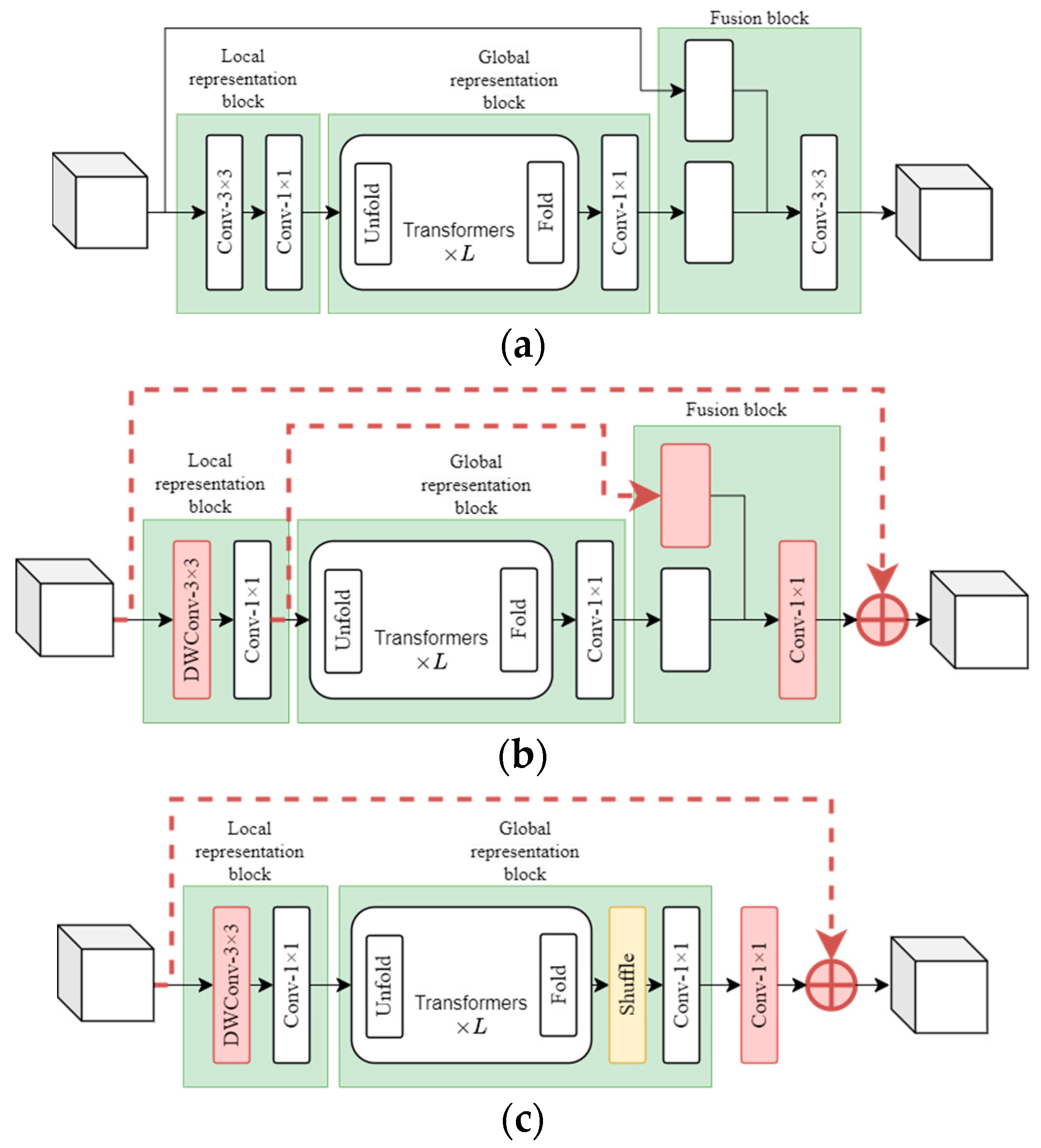
MobileViT is a hybrid CNN-ViT strategy. The general ViT structure is as follows: first a number of patches are obtained based on a partition of the input image; each individual patch is then mapped into a one-dimensional vector via linear variation, which is regarded as a token. Then, the position bias information with learnable parameters is added, and it is processed next by the same number of transformers, and finally the final prediction output is obtained by a layer that is fully connected, and the target is classified according to individual class tokens. The MobileViT structure is shown in Figure 3.
For a given input feature map , its local spatial information is encoded by a convolutional layer with a 3 × 3 convolutional kernel, and then a projection is applied to map the tensor to a high d-dimensional space with a 1 × 1 convolutional layer. At this time, the shape of the feature map is . Global feature modeling is then performed through the transformer structure; in order to enable MobileViT to obtain global representations that contain spatial inductive bias, it unfolds into non-overlapping flat patches , where , , is the patch number, is the patch height, and is the patch width. is the pixel feature in the p-th position for each patch, and the inter-patch relationship is encoded by the transformer to obtain the global feature sequence , as shown in Equation (7).
Unlike the original transformer, MobileViT retains information on both the patch order and the spatial order of the pixels a patch contains (Figure 4). Therefore, we can fold to obtain . is then resized back to its original size in low c-dimensional space using a convolution kernel of 1 × 1 and connected in a series with input via shortcut branches. These connected feature maps are then fused with another 3 × 3 convolutional layer for final output.
Note that for the unfolded feature map , it is generally spread as a sequence, then input into the transformer, and at the time of self-attention, each pixel in the feature map and the other pixels are processed, so that the amount of computation is . In MobileViT, patches are first generated based on a partition of the input feature map, and then the self-attention is calculated only for pixels in the same location of each individual patch, as shown in Figure 4. Here, a patch is represented by a cell surrounded by black lines, while a pixel is represented by a cell surrounded by gray lines. A transformer is utilized to associate the red pixel in the center with blue pixels. Due to the fact that the information of their neighboring pixels has been encoded by blue pixels with convolution, the transformer is able to incorporate the pixel information of all patches in Figure 4. At this time, the amount of computation is reduced to . Since uses convolution to encode localized information from within a 3 × 3 region, and encodes global information for the p-th position of each patch, any pixel included in contains information obtained based on all pixels from .
Our MobileViTSF is a simple and effective modification of MobileViT, as shown in Figure 3c. Its biggest modification is the addition of channel shuffle block in the global representation block. We hope that the shuffle operation on transformer processing can compensate for the degradation of detection performance caused by depthwise separable convolution, while improving the expression of features. We refer to MobileViTv3 and use a depthwise convolutional layer to replace the convolutional layer in the local representation block. We also use 1 × 1 convolutional layers instead of 3 × 3 convolutional layers to simplify the structure of the fusion block. Compared with MobileViT, our method maintains high detection performance with fewer FLOPS and parameters.
3.2.2. Small Target Detection Layer
Due to the fact that some targets are of small sizes, and YOLOv8 has a large down-sampling rate, obtaining feature information for small targets from deeper maps of features is difficult, so the original YOLOv8 model has poor detection ability for targets of small sizes. The original model has a detection scale of 80 × 80 for small targets, and the sensory field obtained from detecting each grid is 8 × 8. In cases where the target in the input image has heights and widths no larger than 8 pixels, the original network has difficulties recognizing the feature information of the target in the grid [46]. Therefore, as Figure 2 shows, the proposed model contains a small target detection layer. A 160 × 160 layer is added to the original network, which includes a complementary fusion feature layer as well as the introduction of additional detection heads, in order to obtain more accurate feature representation and semantic information for targets of small sizes. Firstly, the feature layer with a scale of 80 × 80 (P3) continues to be stacked in the neck, and the feature layer with deep semantic feature information of small targets is constructed after the up-sampling process. It then continues to be spliced with a MobileNetv2 (P2) feature layer with a scale of 160 × 160 in the 4-th layer of the backbone, to supplement and enhance the expression capability of the fusion feature layer for the location information and semantic features of small targets. Then, the 160×160 fusion feature layer is incorporated into the C2f block to improve the expression capability for the semantic features and location information of small targets. The fusion feature layer with a scale of 160 × 160 is sent to the next Conv (convolution) block and an additional detection head after the C2f block.
The addition of the 160 × 160 scale layer allows the information for features of small targets to continue to be passed along the down-sampling path to the other 3 scale feature layers, thus strengthening the capability of the model for the fusion of features and improving the accuracy of small target detection. Introducing an additional decoupling header expands the detection range for ships of small sizes. The improvement in detection accuracy as well as range allows the network to more accurately recognize ships in the river channel.
3.2.3. GSConv
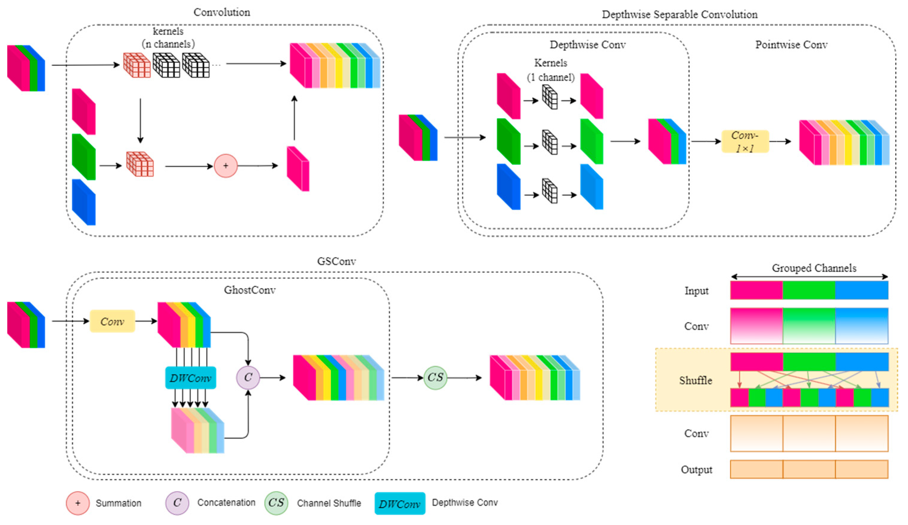
Slim-neck was first applied to vision systems for unmanned vehicles. Its core idea is to keep the excellent and reliable backbone while slimming the neck, which leads to a reduced model size and maintains the detection accuracy. The structure of GSConv in Slim-neck is shown in Figure 5, which incorporates the lightweight idea of GhostNet [47] and ShuffleNetv2 [48]. GhostNet mainly solves the problem that the output of standard convolution usually has many similar feature maps, which can bring redundancy to the computation. Instead of standard convolution, ghost convolution from GhostNet first uses standard convolution to obtain the first part. This part is then convolved via depthwise convolution to get several similar feature maps as the result of the second part. Finally, the two parts are concatenated together as the output feature map. ShuffleNetv2 mainly addresses the fact that the channel information in the depthwise separable convolutional input feature maps is separated during computation, and therefore the information interaction between the channels is separated from each other. Channel shuffle is to shuffle the feature maps along the direction of the channels, using a lower computational cost to make the information between the channels interact with each other.
In this paper, as shown in Figure 2, the GSC2f (gfriend simulator CSPBottleneck with 2 convolutions) structure is further designed on the basis of GSConv. Specifically, GSConv blocks are used instead of the Conv blocks in the neck network, and the original C2f blocks are replaced with the GSC2f blocks for a reduced computational complexity.
4. Experiments
4.1. Dataset Production
The SeaShips dataset was captured using surveillance cameras near the Island of Hengqin in Zhuhai, Guangdong Province of China. Its public part consists of 7000 annotated images. It contains images for 6 types of ships, including passenger ships, container ships, bulk cargo ships, ore carriers and fishing boats. Different ship monitoring situations are covered: different hull sections, proportions, viewing angles and lighting in complex environments and with different levels of occlusion. In addition, we also collected 500 images of the same category for labeling and formed a new dataset with SeaShips; Figure 6 shows the number of instances and the size of ground truths. A total of 80% of the dataset was chosen for training, and the remaining 20% was used for validation. Figure 7 gives actual examples for each category in SeaShips.
4.2. Experimental Configuration
The hardware and software environments in the experiment were configured as follows. An NVIDIA RTX 3090 GPU (made by the NVIDIA Corporation, Santa Clara, CA, USA) with a video memory of 24 GB was used along with a 12-core Intel(R) Xeon(R) Platinum 8255C processor (made by the Intel Corporation, Santa Clara, CA, USA) with 45 GB of RAM (made by Kingston, Fountain Valley, CA, USA) for the computation tasks in testing. The runtime environment is 64-bit ubuntu 18.04, configured with Cuda 11.1, PyTorch 1.9.0 and Python 3.8.
The following parameters are used for the experiments. The optimizer uses SGD: a value of 0.01 is chosen for learning rate, a value of 0.937 is chosen for momentum, and the weight decay is set to be 0.0005. To achieve a balance for the number of sample types, the mixup and mosaic augmentation is set to be 0.1. Due to hardware limitations, the batch size is set to be 8, and the number of train epochs is chosen to be 300.
4.3. Model Evaluation Indicators
Evaluation indicators are essential for the assessment of model performance. In examining the effectiveness of the proposed approach, this paper focuses on precision, recall, FLOPs (floating-point operations), mAP (mean average precision), model size and FPS (frames per second) as measures of algorithm performance. Precisions and recalls are calculated with Equations (8) and (9).
where , , and represent the values of false negative, false positive and true positive, respectively. The mAP metric is based on a precision–recall metric that deals with multiple object classes and defines positive predictions using (intersection over union). It chooses a given threshold of and calculates the mean of the precision values obtained at different recall levels for the threshold. is a measure of the similarity of two sets and is a metric commonly used in computer vision and image processing to numerically evaluate the degree of overlap for two bounding boxes (or two regions):
The (average precision) for a particular category is obtained by ranking the predictions of a model with the values of recalls and calculating the area enclosed by a line generated with precisions represented by the vertical axis and recalls by the horizontal axis in a cartesian coordinate system.
0.5 is the value of when the threshold has a value of 0.5. The for each threshold value from 0.5 to 0.95 with an increment step of 0.05 is calculated and averaged to obtain 0.5:0.95.
The value of is 10. By using 0.5 and 0.5:0.95, we evaluate the capability of the model for accurate detection of ships at various thresholds. In addition, the performance of the proposed model is also described by its number of parameters and the FLOPs, which represent the amount of computation needed by the model and measure the model complexity. The model size can reflect the number of parameters the model contains. For real-world applications, we also consider the number of FPS.
5. Results and Discussion
5.1. Ablation Experiments
In order to test the effectiveness of the improved method in this paper, ablation experiments are performed with the same training strategy and hyperparameters. As can be seen from Table 1, in cases where only a replacement of the backbone is implemented, the FLOPs and model size decrease significantly, while the model performance decreases slightly. When changing only the neck structure and adding a large-scale detection layer, the model’s detection rises significantly, as does the amount of computation for the model. When using only the lightweight GSConv block and the GSC2f block, the model’s mAP0.5:0.95 rises slightly, and FLOPs (floating-point operations per second) and model size decrease. In cases where both the backbone structure is replaced and the lightweight neck is used, the model’s computation and size decrease substantially with increased values of mAP. Compared to the original YOLOv8, the final model with all three improvements combined achieves improvements of 0.9% and 4.5% in mAP0.5 and mAP0.5:0.95, respectively, while the GFLOPs (giga floating-point operations per second) decrease by 51.9%, and the model size decreases by 41.9%.
5.2. Comparison Experiments
This part compares the experimental results obtained with the proposed approach with those of several other state-of-the-art lightweight methods for target detection on the SeaShips dataset. Table 2 shows that the proposed approach achieves performance better than that of other tested methods in terms of mAP, computation amount and model size. In Table 3, we make a comparison between the mAP of YOLOv8n and our method in each ship’s category.
The mAP0.5 and mAP0.5:0.95 of our proposed algorithms improve 4.4% and 12.5% compared to the YOLOv7-tiny algorithm, 6.7% and 5.7% compared to the YOLOX-s algorithm, 0.8% and 3.8% compared to the YOLOv6 algorithm, and 1.1% and 8% compared to the 6.0 version of YOLOv5 in 2021. Our model that also incorporates a P2 layer in YOLOv5 is also compared, with mAP0.5 and mAP0.5:0.95 improving by 0.6% and 1.6%, respectively. Our model still outperforms the earlier tiny models of YOLOv3 and YOLOv4.
Compared to the original Slim-neck, our method improves mAP0.5 and mAP0.5:0.95 by 0.8% and 4.8%, respectively. Compared to the minimalist-structured VanillaNet, the proposed model improves on mAP0.5 and mAP0.5:0.95 by 2% and 9.2%. Our algorithm also outperforms the architecture where MobileViT and MobileViTv3 are added to YOLOv8. Our model has the smallest FLOPs, and the model size is only slightly larger than that of MobileViT and MobileViTv3. Due to the addition of a large-scale detection layer, some of the detection speed is sacrificed, but the FPS on the GPU is over 60, which is sufficient for the human eye. A comparison of these models on detection performance suggests that the proposed model is computationally efficient and has higher detection accuracy.
5.3. Experimental Analysis
The performance of the proposed model is also compared with that of the YOLOv8n model. Figure 8 shows a comparison of the recognition results for small ship targets where the heat map was generated using Grad-CAM (gradient-weighted class activation mapping) [50]. The original YOLOv8n did not detect ships that were far away from the camera and small ships that appeared between larger ships. As the heat map demonstrates, our method incorporates a large-scale small target detection layer. As a result, higher weights are generated for these small targets after shallow features are fused. These small ship targets can thus be detected using the proposed approach.
We also show the results of target detection in other scenarios. YOLOv8n tends to miss and generate false detection results when images with more complex backgrounds need to be processed, especially in blurred images where different types of ships overlap with one another. For example, Figure 9 demonstrates a case where ships overlap, and the overlapping part of the large ship is recognized with YOLOv8n as a false target. YOLOv8n may generate false detection results under foggy weather and complex backgrounds. In contrast, the algorithm proposed in this paper incorporates a visual transformer MobileViTSF and a large-scale small target detection layer, which can locate the target with high accuracy and reduce the rate of false detections effectively. Therefore, the proposed approach achieves higher detection accuracy and detection speed while maintaining a smaller size, which can meet the practical needs of real-time detection.
6. Conclusions
This paper proposes a new YOLOv8 detection model to support port management and vessel monitoring. To improve the reliability of the model for the detection of ship targets in river traffic situations, a MobileViTSF block is added to the backbone network, which can capture the most discriminative regions in the complex river background image by using the global information learning capability of the visual transformer, making the model focus on the target rather than the background. To enhance the ability of the model to accurately obtain features for small target vessels, we redesigned the neck network by adding a shallow feature fusion layer of 160 × 160 size and a corresponding detection head. To make the network lightweight and ensure detection effectiveness, GSConv is employed, and the C2f block in YOLOv8 is redesigned, which leads to a significantly reduced model size and computational complexity. The improved model improves mAP0.5 and mAP0.5:0.95 by 0.9% and 5.5%, respectively. Compared to the original model, a reduction of 51.9% is achieved for the GFLOPs, and the size of the model is reduced by 41.9%, which achieves improved detection performance and lower computational cost. The testing results show that the proposed method outperforms several state-of-the-art target detection models in detection accuracy. It can meet the requirements of reliable, accurate and fast target detection for ship identification and surveillance.
However, the proposed method still has some shortcomings. For example, when a certain number of large ships overlap with one another, the detection accuracy of our proposed model will be adversely affected, and the FPS still has room to increase. For future research, the proposed model will be continuously improved so that it can achieve higher detection accuracy and detection speed. Considering the practical value of this approach in real-time applications, the proposed model can also be ported to mobile edge platforms (such as mobile phones and NVIDIA Jetson series).
Author Contributions
Conceptualization, X.Z. and Y.S.; methodology, X.Z.; software, X.Z.; validation, X.Z. and Y.S.; formal analysis, X.Z.; resources, X.Z.; data curation, X.Z.; writing—original draft preparation, X.Z.; writing—review and editing, Y.S.; visualization, X.Z.; supervision, Y.S. All authors have read and agreed to the published version of the manuscript.
Funding
This research is fully supported by the University Research Funding Project of Jiangsu University of Science and Technology, under the grant number 1132921208.
Data Availability Statement
The data reported in this paper are freely available upon reasonable request.
Conflicts of Interest
The authors declare no conflict of interest.
References
- Chen, P.; Li, X.; Zheng, G. Rapid detection to long ship wake in synthetic aperture radar satellite imagery. J. Oceanol. Limnol. 2019, 37, 1523–1532. [Google Scholar] [CrossRef]
- Wu, W.; Li, X.; Hu, Z.; Liu, X. Ship Detection and Recognition Based on Improved YOLOv7. Comput. Mater. Contin. 2023, 76, 1. [Google Scholar] [CrossRef]
- Yu, N.; Fan, X.; Deng, T.; Mao, G. Ship detection algorithm with complex background based on multi-head self-attention. J. Zhejiang Univ. Eng. Ed. 2022, 12, 2392–2402. [Google Scholar]
- Lee, S.J.; Roh, M.I.; Lee, H.W.; Ha, J.S.; Woo, I.G. Image-Based Ship Detection and Classification for Unmanned Surface Vehicle using Real-Time Object Detection Neural Networks. In Proceedings of the ISOPE International Ocean and Polar Engineering Conference, ISOPE, Sapporo, Japan, 10–15 June 2018. [Google Scholar]
- Shao, Z.; Wang, L.; Wang, Z.; Du, W.; Wu, W. Saliency-aware convolution neural network for ship detection in surveillance video. IEEE Trans. Circuits Syst. Video Technol. 2019, 30, 781–794. [Google Scholar] [CrossRef]
- Ting, L.; Baijun, Z.; Yongsheng, Z.; Shun, Y. Ship Detection Algorithm Based on Improved YOLO V5. In Proceedings of the 2021 6th International Conference on Automation, Control and Robotics Engineering (CACRE), Dalian, China, 15–17 July 2021; pp. 483–487. [Google Scholar]
- Li, H.; Deng, L.; Yang, C.; Liu, J.; Gu, Z. Enhanced YOLO v3 tiny network for real-time ship detection from visual image. IEEE Access 2021, 9, 16692–16706. [Google Scholar] [CrossRef]
- Xie, P.; Tao, R.; Luo, X.; Shi, Y. YOLOv4-MobileNetV2-DW-LCARM: A Real-Time Ship Detection Network. In Communications in Computer and Information Science, Proceedings of the International Conference on Knowledge Management in Organizations, Hagen, Germany, 11–14 July 2022; Springer International Publishing: Cham, Switzerland, 2022; pp. 281–293. [Google Scholar]
- Shao, Z.; Wu, W.; Wang, Z.; Du, W.; Li, C. Seaships: A large-scale precisely annotated dataset for ship detection. IEEE Trans. Multimed. 2018, 20, 2593–2604. [Google Scholar] [CrossRef]
- Chen, J.; Wang, J.; Lu, H. Ship Detection in Complex Weather Based on CNN. In Proceedings of the 2021 6th International Conference on Intelligent Computing and Signal Processing (ICSP), Xi’an, China, 9–11 April 2021; pp. 1225–1228. [Google Scholar]
- Han, X.; Zhao, L.; Ning, Y.; Hu, J. ShipYolo: An enhanced model for ship detection. J. Adv. Transp. 2021, 2021, 1–11. [Google Scholar] [CrossRef]
- Terven, J.; Cordova-Esparza, D. A comprehensive review of YOLO: From YOLOv1 to YOLOv8 and beyond. arXiv 2023, arXiv:2304.00501. [Google Scholar]
- Mehta, S.; Rastegari, M. Mobilevit: Light-weight, general-purpose, and mobile-friendly vision transformer. arXiv 2021, arXiv:2110.02178. [Google Scholar]
- Wadekar, S.N.; Chaurasia, A. Mobilevitv3: Mobile-friendly vision transformer with simple and effective fusion of local, global and input features. arXiv 2022, arXiv:2209.15159. [Google Scholar]
- Li, H.; Li, J.; Wei, H.; Liu, Z.; Zhan, Z.; Ren, Q. Slim-neck by GSConv: A better design paradigm of detector architectures for autonomous vehicles. arXiv 2022, arXiv:2206.02424. [Google Scholar]
- Lowe, G. Sift-the scale invariant feature transform. Int. J. 2004, 2, 2. [Google Scholar]
- Dalal, N.; Triggs, B. Histograms of Oriented Gradients for Human Detection. In Proceedings of the 2005 IEEE Computer Society Conference on Computer Vision and Pattern Recognition (CVPR’05), San Diego, CA, USA, 20–25 June 2005; Volume 1, pp. 886–893. [Google Scholar]
- Forsyth, D. Object detection with discriminatively trained part-based models. Computer 2014, 47, 6–7. [Google Scholar] [CrossRef]
- Neubeck, A.; Van Gool, L. Efficient Non-Maximum Suppression. In Proceedings of the 18th International Conference on Pattern Recognition (ICPR’06), Hong Kong, China, 20–24 August 2006; Volume 3, pp. 850–855. [Google Scholar]
- Girshick, R.; Donahue, J.; Darrell, T.; Malik, J. Rich Feature Hierarchies for Accurate Object Detection and Semantic Segmentation. In Proceedings of the IEEE Conference on Computer Vision and Pattern Recognition, Columbus, OH, USA, 23–28 June 2014; pp. 580–587. [Google Scholar]
- Girshick, R. Fast r-cnn. In Proceedings of the IEEE International Conference on Computer Vision, Santiago, Chile, 7–13 December 2015; pp. 1440–1448. [Google Scholar]
- Ren, S.; He, K.; Girshick, R.; Sun, J. Faster r-cnn: Towards real-time object detection with region proposal networks. In Proceedings of the Advances in Neural Information Processing Systems, Montreal, QC, Canada, 7–12 December 2015; Volume 28. [Google Scholar]
- Pang, J.; Chen, K.; Shi, J.; Feng, H.; Ouyang, W.; Lin, D. Libra r-cnn: Towards Balanced Learning for Object Detection. In Proceedings of the IEEE/CVF Conference on Computer Vision and Pattern Recognition, Long Beach, CA, USA, 15–20 June 2019; pp. 821–830. [Google Scholar]
- Redmon, J.; Divvala, S.; Girshick, R.; Farhadi, A. You Only Look Once: Unified, Real-Time Object Detection. In Proceedings of the IEEE Conference on Computer Vision and Pattern Recognition, Las Vegas, NV, USA, 27–30 June 2016; pp. 779–788. [Google Scholar]
- Redmon, J.; Farhadi, A. YOLO9000: Better, Faster, Stronger. In Proceedings of the IEEE Conference on Computer Vision and Pattern Recognition, Honolulu, HI, USA, 21–26 July 2017; pp. 7263–7271. [Google Scholar]
- Redmon, J.; Farhadi, A. Yolov3: An incremental improvement. arXiv 2018, arXiv:1804.02767. [Google Scholar]
- He, K.; Zhang, X.; Ren, S.; Sun, J. Deep Residual Learning for Image Recognition. In Proceedings of the IEEE Conference on Computer Vision and Pattern Recognition, Las Vegas, NV, USA, 27–30 June 2016; pp. 770–778. [Google Scholar]
- Lin, T.Y.; Dollár, P.; Girshick, R.; He, K.; Hariharan, B.; Belongie, S. Feature Pyramid Networks for Object Detection. In Proceedings of the IEEE Conference on Computer Vision and Pattern Recognition, Honolulu, HI, USA, 21–26 July 2017; pp. 2117–2125. [Google Scholar]
- Bochkovskiy, A.; Wang, C.Y.; Liao, H.Y.M. Yolov4: Optimal speed and accuracy of object detection. arXiv 2020, arXiv:2004.10934. [Google Scholar]
- Zheng, Z.; Wang, P.; Ren, D.; Liu, W.; Ye, R.; Hu, Q.; Zuo, W. Enhancing geometric factors in model learning and inference for object detection and instance segmentation. IEEE Trans. Cybern. 2021, 52, 8574–8586. [Google Scholar] [CrossRef]
- Ge, Z.; Liu, S.; Wang, F.; Li, Z.; Sun, J. Yolox: Exceeding yolo series in 2021. arXiv 2021, arXiv:2107.08430. [Google Scholar]
- Tan, M.; Pang, R.; Le, Q.V. Efficientdet: Scalable and Efficient Object Detection. In Proceedings of the IEEE/CVF Conference on Computer Vision and Pattern Recognition, Seattle, WA, USA, 13–19 June 2020; pp. 10781–10790. [Google Scholar]
- Cui, Y.; Yang, L.; Liu, D. Dynamic proposals for efficient object detection. arXiv 2022, arXiv:2207.05252. [Google Scholar]
- Jung, H.K.; Choi, G.S. Improved yolov5: Efficient object detection using drone images under various conditions. Appl. Sci. 2022, 12, 7255. [Google Scholar] [CrossRef]
- Zhao, J.; Xu, S.; Wang, R.; Zhang, B.; Guo, G.; Doermann, D.; Sun, D. Data-adaptive binary neural networks for efficient object detection and recognition. Pattern Recognit. Lett. 2022, 153, 239–245. [Google Scholar] [CrossRef]
- Vaswani, A.; Shazeer, N.; Parmar, N.; Uszkoreit, J.; Jones, L.; Gomez, A.N.; Polosukhin, I. Attention is all you need. In Proceedings of the Advances in Neural Information Processing Systems, Long Beach, CA, USA, 4–9 December 2017; Volume 30. [Google Scholar]
- Carion, N.; Massa, F.; Synnaeve, G.; Usunier, N.; Kirillov, A.; Zagoruyko, S. End-to-End Object Detection with Transformers. In Lecture Notes in Computer Science, Proceedings of the European Conference on Computer Vision, Glasgow, UK, 23–28 August 2020; Springer International Publishing: Cham, Switzerland, 2020; pp. 213–229. [Google Scholar]
- Dosovitskiy, A.; Beyer, L.; Kolesnikov, A.; Weissenborn, D.; Zhai, X.; Unterthiner, T.; Houlsby, N. An image is worth 16 × 16 words: Transformers for image recognition at scale. arXiv 2020, arXiv:2010.11929. [Google Scholar]
- Liu, Z.; Lin, Y.; Cao, Y.; Hu, H.; Wei, Y.; Zhang, Z.; Guo, B. Swin Transformer: Hierarchical Vision Transformer using Shifted Windows. In Proceedings of the IEEE/CVF International Conference on Computer Vision, Montreal, BC, Canada, 11–17 October 2021; pp. 10012–10022. [Google Scholar]
- Li, Y.; Mao, H.; Girshick, R.; He, K. Exploring Plain Vision Transformer Backbones for Object Detection. In Lecture Notes in Computer Science, Proceedings of the European Conference on Computer Vision, Tel Aviv, Israel, 23–27 October 2022; Springer Nature: Cham, Switzerland, 2022; pp. 280–296. [Google Scholar]
- Wang, C.Y.; Bochkovskiy, A.; Liao, H.Y.M. YOLOv7: Trainable Bag-of-Freebies Sets New State-of-the-Art for Real-Time Object Detectors. In Proceedings of the IEEE/CVF Conference on Computer Vision and Pattern Recognition, Vancouver, BC, Canada, 18–22 June 2023; pp. 7464–7475. [Google Scholar]
- Liu, S.; Qi, L.; Qin, H.; Shi, J.; Jia, J. Path Aggregation Network for Instance Segmentation. In Proceedings of the IEEE Conference on Computer Vision and Pattern Recognition, Salt Lake City, UT, USA, 18–23 June 2018; pp. 8759–8768. [Google Scholar]
- Feng, C.; Zhong, Y.; Gao, Y.; Scott, M.R.; Huang, W. Tood: Task-Aligned One-Stage Object Detection. In Proceedings of the 2021 IEEE/CVF International Conference on Computer Vision (ICCV), Montreal, BC, Canada, 11–17 October 2021; IEEE Computer Society: Washington, DC, USA, 2021; pp. 3490–3499. [Google Scholar]
- Li, X.; Wang, W.; Wu, L.; Chen, S.; Hu, X.; Li, J.; Yang, J. Generalized focal loss: Learning qualified and distributed bounding boxes for dense object detection. Adv. Neural Inf. Process. Syst. 2020, 33, 21002–21012. [Google Scholar]
- Sandler, M.; Howard, A.; Zhu, M.; Zhmoginov, A.; Chen, L.C. Mobilenetv2: Inverted Residuals and Linear Bottlenecks. In Proceedings of the IEEE Conference on Computer Vision and Pattern Recognition, Salt Lake City, UT, USA, 18–22 June 2018; pp. 4510–4520. [Google Scholar]
- Xiong, E.; Zhang, R.; Liu, Y.; Peng, J. Ghost-YOLOv8 detection algorithm for traffic signs. IN Comput. Eng. Appl. 2023, 59, 200–207. [Google Scholar]
- Han, K.; Wang, Y.; Tian, Q.; Guo, J.; Xu, C.; Xu, C. Ghostnet: More Features from Cheap Operations. In Proceedings of the IEEE/CVF Conference on Computer Vision and Pattern Recognition, Seattle, WA, USA, 13–19 June 2020; pp. 1580–1589. [Google Scholar]
- Ma, N.; Zhang, X.; Zheng, H.T.; Sun, J. Shufflenet v2: Practical Guidelines for Efficient cnn Architecture Design. In Proceedings of the European Conference on Computer Vision (ECCV), Munich, Germany, 8–14 September 2018; pp. 116–131. [Google Scholar]
- Chen, H.; Wang, Y.; Guo, J.; Tao, D. VanillaNet: The Power of Minimalism in Deep Learning. arXiv 2023, arXiv:2305.12972. [Google Scholar]
- Selvaraju, R.R.; Cogswell, M.; Das, A.; Vedantam, R.; Parikh, D.; Batra, D. Grad-cam: Visual Explanations from Deep Networks via Gradient-Based Localization. In Proceedings of the IEEE International Conference on Computer Vision, Venice, Italy, 22–29 October 2017; pp. 618–626. [Google Scholar]
Figure 1.
YOLOv8 network structure.

Figure 2.
Improved YOLOv8 network structure.

Figure 3.
MobileViT’s structure. (a) MobileViT. (b) MobileViTv3. (c) Our MobileViTSF.

Figure 4.
Local representation and global representation schema.

Figure 5.
Schematic diagram of the different convolution processes and channel shuffle.

Figure 6.
SeaShips dataset details; (a) the instance number for each category in the SeaShips dataset; (b) the size of the GT (ground truth)box for each instance; (c) the coordinates of the midpoint of each GT box; (d) the height and width of each GT box.
Figure 6.
SeaShips dataset details; (a) the instance number for each category in the SeaShips dataset; (b) the size of the GT (ground truth)box for each instance; (c) the coordinates of the midpoint of each GT box; (d) the height and width of each GT box.

Figure 7.
Examples for all categories of ships in the dataset; (a) an example of ore carriers; (b) an example of bulk cargo carriers; (c) an example of general cargo ships;(d) an example of fishing boats; (e) an example of container ships; (f) an example of passenger ships.
Figure 7.
Examples for all categories of ships in the dataset; (a) an example of ore carriers; (b) an example of bulk cargo carriers; (c) an example of general cargo ships;(d) an example of fishing boats; (e) an example of container ships; (f) an example of passenger ships.

Figure 8.
Comparison of heatmaps for small target detection, the tested image on the right contains a Chinese marker generated by the imaging system to indicate the date when the image was obtained; (a) YOLOv8n. (b) Ours.
Figure 8.
Comparison of heatmaps for small target detection, the tested image on the right contains a Chinese marker generated by the imaging system to indicate the date when the image was obtained; (a) YOLOv8n. (b) Ours.

Figure 9.
Comparison of model detection results, all tested images contain two Chinese markers (one is on the top, the other one is on the bottom of the image) generated by the imaging system to show information on when and where the image was obtained; (a) YOLOv8n. (b) Ours.
Figure 9.
Comparison of model detection results, all tested images contain two Chinese markers (one is on the top, the other one is on the bottom of the image) generated by the imaging system to show information on when and where the image was obtained; (a) YOLOv8n. (b) Ours.


Table 1.
Results of the ablation experiment, where a ‘√’ indicates that the corresponding technique is used to construct the model for detection.
Table 1.
Results of the ablation experiment, where a ‘√’ indicates that the corresponding technique is used to construct the model for detection.
| YOLOv8 | MobileViTSF | P2 | GSConv | mAP0.5 (%) | mAP0.5:0.95 (%) | FLOPs (G) | Size (MB) |
|---|---|---|---|---|---|---|---|
| √ | 97.9 | 78.0 | 8.1 | 6.2 | |||
| √ | √ | 97.8 | 76.4 | 4.9 | 2.7 | ||
| √ | √ | 98.5 | 82.3 | 12.2 | 6.5 | ||
| √ | √ | 98.1 | 77.5 | 7.0 | 5.5 | ||
| √ | √ | √ | 98.1 | 80.3 | 1.2 | 2.6 | |
| √ | √ | √ | √ | 98.8 | 82.5 | 3.9 | 3.6 |
Table 2.
The results of the experiments for comparison with other models, a number in bold shows the best performance achieved for each performance index.
Table 2.
The results of the experiments for comparison with other models, a number in bold shows the best performance achieved for each performance index.
| Models | Input | mAP0.5 (%) | mAP0.5:0.95 (%) | FLOPs (G) | Size (MB) | FPS (F/S) |
|---|---|---|---|---|---|---|
| YOLOv8n | 640 × 640 | 97.9 | 78.0 | 8.1 | 6.2 | 102.04 |
| YOLOv7-tiny | 640 × 640 | 94.4 | 70.2 | 13.2 | 12.0 | 66.22 |
| YOLOX-s | 640 × 640 | 92.1 | 76.8 | 26.77 | 8.9 | 94.3 |
| YOLOv6 | 640 × 640 | 98.0 | 78.7 | 11.9 | 8.7 | 83.33 |
| YOLOv5n(6.0) | 640 × 640 | 97.7 | 74.5 | 7.8 | 5.2 | 65.36 |
| YOLOv5n(6.0)-P2 | 1280 × 1280 | 98.2 | 80.9 | 7.2 | 8.7 | 67.11 |
| YOLOv4-tiny | 416 × 416 | 97.1 | 75.2 | 20.8 | 18.6 | 44.64 |
| YOLOv3-tiny | 416 × 416 | 96.8 | 71.4 | 18.9 | 24.4 | 163.98 |
| Slim-neck+v8 | 640 × 640 | 98.0 | 77.7 | 7.0 | 5.5 | 110.48 |
| VanillaNet [49] | 640 × 640 | 96.8 | 73.3 | 10.2 | 7.9 | 96.98 |
| MobileViT+v8 | 640 × 640 | 93.6 | 69.0 | 5.3 | 2.6 | 70.42 |
| MobileViTv3+v8 | 640 × 640 | 95.8 | 74.1 | 5.5 | 2.9 | 72.53 |
| Ours | 1280 × 1280 | 98.8 | 82.5 | 3.9 | 3.6 | 68.49 |
Table 3.
YOLOv8n and our model for each category of mAP.
| Category | YOLOv8n | Ours | ||
|---|---|---|---|---|
| mAP0.5(%) | mAP0.5:0.95(%) | mAP0.5(%) | mAP0.5:0.95(%) | |
| Ore carrier | 98.4 | 75.6 | 98.9 | 81.6 |
| Bulk cargo carrier | 97.8 | 77.2 | 98.8 | 83.9 |
| General cargo carrier | 98.5 | 80.5 | 99.2 | 85.3 |
| Container carrier | 99.0 | 83.7 | 99.5 | 86.7 |
| Fishing boat | 96.1 | 72.4 | 98.0 | 78.7 |
| Passenger ship | 97.3 | 73.0 | 98.6 | 78.9 |
Disclaimer/Publisher’s Note: The statements, opinions and data contained in all publications are solely those of the individual author(s) and contributor(s) and not of MDPI and/or the editor(s). MDPI and/or the editor(s) disclaim responsibility for any injury to people or property resulting from any ideas, methods, instructions or products referred to in the content. |
© 2023 by the authors. Licensee MDPI, Basel, Switzerland. This article is an open access article distributed under the terms and conditions of the Creative Commons Attribution (CC BY) license (https://creativecommons.org/licenses/by/4.0/).
Share and Cite
MDPI and ACS Style
Zhao, X.; Song, Y. Improved Ship Detection with YOLOv8 Enhanced with MobileViT and GSConv. Electronics 2023, 12, 4666. https://doi.org/10.3390/electronics12224666
AMA Style
Zhao X, Song Y. Improved Ship Detection with YOLOv8 Enhanced with MobileViT and GSConv. Electronics. 2023; 12(22):4666. https://doi.org/10.3390/electronics12224666
Chicago/Turabian StyleZhao, Xuemeng, and Yinglei Song. 2023. "Improved Ship Detection with YOLOv8 Enhanced with MobileViT and GSConv" Electronics 12, no. 22: 4666. https://doi.org/10.3390/electronics12224666
Note that from the first issue of 2016, this journal uses article numbers instead of page numbers. See further details here.