Bit-Weight Adjustment for Bridging Uniform and Non-Uniform Quantization to Build Efficient Image Classifiers

Abstract

Network quantization, which strives to reduce the precision of model parameters and/or features, is one of the most efficient ways to accelerate model inference and reduce memory consumption, particularly for deep models when performing a variety of real-time vision tasks on edge platforms with constrained resources. Existing quantization approaches function well when using relatively high bit widths but suffer from a decline in accuracy at ultra-low precision. In this paper, we propose a bit-weight adjustment (BWA) module to bridge uniform and non-uniform quantization, successfully quantizing the model to ultra-low bit widths without bringing about noticeable performance degradation. Given uniformly quantized data, the BWA module adaptively transforms these data into non-uniformly quantized data by simply introducing trainable scaling factors. With the BWA module, we combine uniform and non-uniform quantization in a single network, allowing low-precision networks to benefit from both the hardware friendliness of uniform quantization and the high performance of non-uniform quantization. We optimize the proposed BWA module by directly minimizing the classification loss through end-to-end training. Numerous experiments on the ImageNet and CIFAR-10 datasets reveal that the proposed approach outperforms state-of-the-art approaches across various bit-width settings and can even produce low-precision quantized models that are competitive with their full-precision counterparts.

1. Introduction

The past decade has witnessed the astonishing evolution of deep learning techniques. The success of deep learning models, especially convolutional neural networks (CNNs) [1,2], has dramatically facilitated the advancement of computer vision and graphics, making CNNs the primary tool within the community of computational visual media. To date, CNNs have made remarkable achievements across a wide range of vision tasks and applications such as person identification [3], object detection [4], action recognition [5], and image classification [6].

However, although the performance of CNNs has pushed the limits, the runtime overhead is another critical factor to take into consideration in practice. Generally, the remarkable achievements of CNNs come from the huge model sizes and the tremendous number of parameters. Typical modern CNNs involve billions of FLOPs, leading to high latency, significant resource requirements, and substantial energy consumption. This makes it impractical for CNNs to execute various real-time vision tasks on edge or mobile platforms with limited resources. With the ever-increasing number of embedded and mobile devices that require vision or graphics processing, the CNN deployment challenge has risen to the forefront.

To address this challenge, a large number of studies on model compression techniques have emerged, such as efficient model architecture design [7], network pruning [8], knowledge distillation [9], and quantization [10]. Among these approaches, quantization, which aims to leverage low-bit values to encode the original full-precision parameters and/or features of CNN models, has shown great success and is attracting increasing interest.

A host of quantization methods have been studied to achieve compression and acceleration of CNNs, which can typically be divided into two categories: uniform quantization and non-uniform quantization. Most existing methods like [11,12] focus on uniform quantization because they encode data using hardware-friendly fixed-point integers [10]. However, uniformly spaced quantization levels lead to a noticeable decline in accuracy because of the non-uniform distributions of the data of CNNs. To mitigate this problem, research on non-uniform quantization has emerged. Works like [13,14,15] suggest achieving quantization by encoding the target data utilizing multiple binary encodes together with the corresponding coefficients. Such an encoding scheme endows the quantized data with a stronger representation capability and makes the quantization levels fit the data distribution better. Therefore, these methods can usually achieve higher accuracy compared to uniform quantization methods. However, the integer optimization involved in these methods makes the quantization problem NP-hard. They leverage an alternating updating strategy to train the binary encodes and corresponding coefficients, incurring heavy computational loads during training. Additionally, the trained floating-point coefficients also introduce extra computational overheads in the inference procedure.

In this paper, we introduce a novel bit-weight adjustment (BWA) module to learn the best quantization schemes for each layer to boost the performance of quantized models. The BWA module builds on the idea that quantization levels can be optimized by adjusting the weight of each bit. As shown in Figure 1, the BWA module transforms uniformly spaced quantization levels into non-uniformly spaced forms by simply introducing a trainable scaling factor ${\alpha }_i$ to each bit $b_i$. With the BWA module, we can easily obtain the best quantization schemes for different layers through end-to-end training. In contrast to prior research that attempted to reduce reconstruction errors [13,14], we derive the optimal scaling factors of each BWA module by directly minimizing the task loss, which assists in retaining model accuracy after quantization [15,16]. Additionally, in order to benefit from both the hardware friendliness of uniform quantization and the high performance of non-uniform quantization, we propose to combine uniform quantization and non-uniform quantization in a single network. Specifically, we only apply the BWA module to the last few quantization layers of a neural network. The remaining layers are quantized using simple uniform quantization.

The contributions of this paper can be summarized as follows:

• We introduce the BWA module to learn the best quantization schemes for each layer, which can be easily optimized through end-to-end training using two different training strategies: incremental training and joint training.
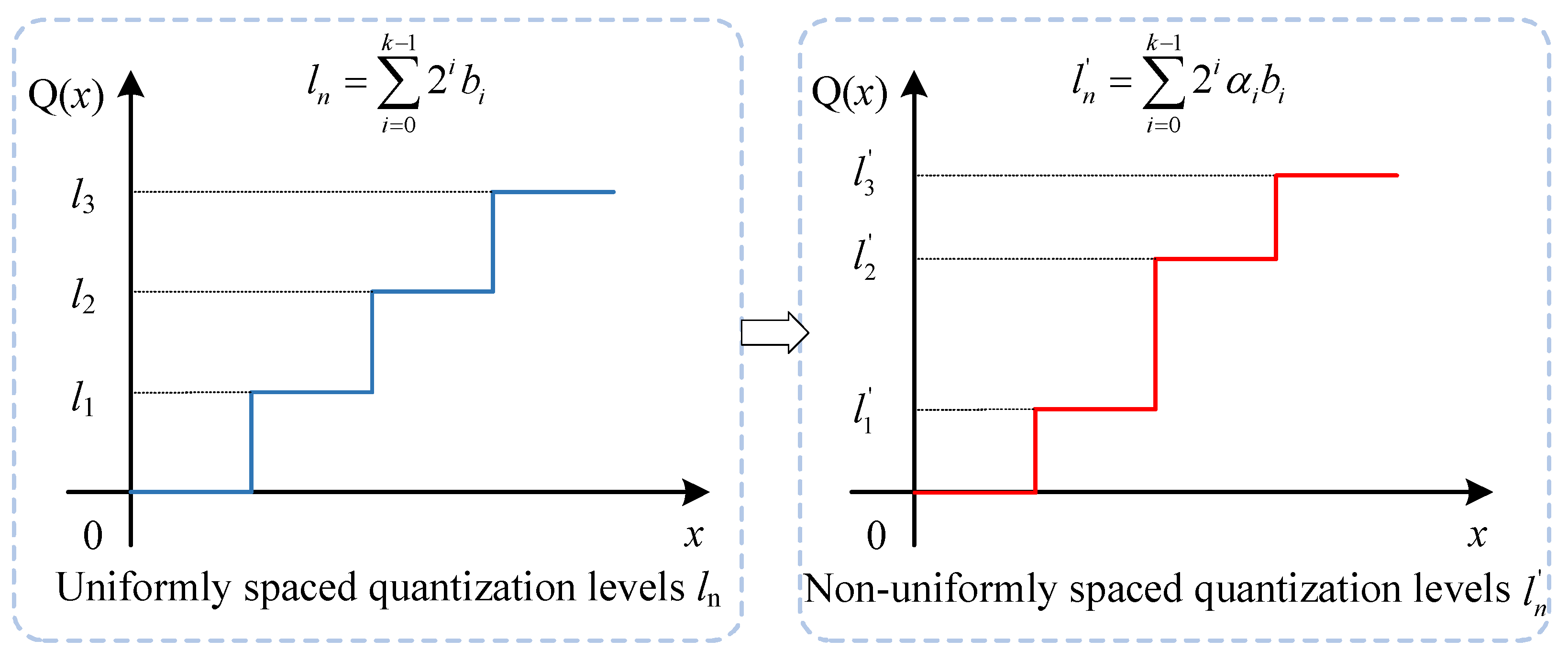
• We combine uniform and non-uniform quantization to benefit from both the hardware friendliness of uniform quantization and the high performance of non-uniform quantization.
• Numerous experiments are performed to verify the performance of our proposed quantization technique. Specifically, our approach sets a new state of the art on the standard benchmark datasets ImageNet [17] and CIFAR-10 [18].

2. Related Works

Research on quantization is an emerging topic and shows great potential for the deployment of CNNs on resource-limited devices. A large number of quantization techniques to achieve model compression have emerged. These methods adopt either uniform quantization schemes or non-uniform quantization schemes. In this section, we review some representative works that have recently been published on the topic of both uniform and non-uniform quantization.

Uniform quantization, which linearly maps floating-point data to some integers, is the most commonly used quantization scheme. Zhou et al. [10] designed DoReFa-Net to achieve arbitrary bit widths in weights, activations, and gradients. In their work, the weights and activations of models are quantized with deterministic quantization, whereas the low-bit-width gradients are obtained through stochastic quantization. Choi et al. [11] concentrated on the quantization of activations and parameterized the activation clipping upper bound to reduce the quantization error through training. They obtained 4-bit quantized models that are comparable to full-precision models in terms of accuracy. Gong et al. [12] proposed to approximate standard uniform quantization with a series of hyperbolic tangent functions. This made the quantization process differentiable, and it could thus mitigate the mismatch of gradients. Dong et al. [19] allocated different bit widths to different layers to boost model performance. Specifically, they leveraged the average Hessian trace to measure the quantization sensitivity to determine the bit width of each layer. Lee et al. [20] attempted to address the quantization problem from the aspect of backpropagation and tried to eliminate the mismatch of gradients using the Taylor approximation.

For non-uniform quantization methods, the intervals between adjacent quantization levels can be different. In [21,22,23,24,25], model weights and activations were coded using logarithmic quantizers. The base-2 logarithmic representation was used due to its compatibility with the bit-shift operation. However, these approaches focused too much on near-zero regions and ignored other regions, thus suffering from a decline in accuracy. Another branch of non-uniform quantization is multi-bit quantization, where the target data are quantized using multiple binary codes. For example, Zhang et al. [13] proposed training quantization levels together with model parameters to minimize quantization errors. Lin et al. [14] proposed obtaining the quantization scheme by minimizing the least-square error. Qu et al. [15] leveraged an iterative optimization strategy to learn the quantization strategy. Xu et al. [26] used an alternating minimization strategy to tackle the quantization problem in LSTM. Li et al. [27] proposed performing recursive residual quantization to obtain a series of binary codes. Owing to their stronger representation capability, these methods usually exhibited better performance compared to uniform quantization methods. However, the floating-point coordinates used in these methods introduced extra computational overhead compared to uniform quantization.

Unlike the methods mentioned above, our work combines uniform and non-uniform quantization to pursue higher accuracy while reducing computational complexity.

3. Preliminary

This section first introduces the goal of the quantization of CNNs. Subsequently, the theoretic basis for the computational acceleration of CNNs through quantization is detailed.

3.1. Network Quantization

The number of parameters included in modern CNNs is typically in the millions, leading to a huge consumption of memory. In addition, the large amount of computationally expensive floating-point operations performed between model parameters and hidden feature maps imposes a huge overhead on computational resources. The significant consumption of memory and computing resources severely limits the widespread use of CNNs on IoT devices with constrained resources.

The goal of network quantization is to slim the size of models and accelerate the computations by encoding the original 32-bit model weights $\mathit{W}$ and activations $\mathit{A}$ using low-precision values. Generally, quantization can be expressed as a piecewise mapping function, as follows:

$$Q\left(x\right)=l_n,\mathrm{if}x\in (s_n,s_{n+1}]$$

(1)

where $l_n$ is the n-th quantization level and $s_n$ and $s_{n+1}$ denote the corresponding quantization steps. For k-bit quantization, there are $2^k$ discrete quantization levels in total. This quantization function maps input data to a quantization level $l_n$ when it falls between $s_n$ and $s_{n+1}$. It should be noted that the quantization levels and the steps can be spaced uniformly or non-uniformly. The most commonly utilized setting is uniform quantization, which utilizes evenly spaced quantization levels and steps.

3.2. Computational Acceleration

Using a low bit width to encode model weights can significantly reduce the model’s size. Quantizing model weights to k bits can compress the model’s size by roughly $\frac{32}{k}$ times compared to the typical 32-bit full-precision counterpart. Furthermore, when we properly encode both the model weights and activations using low-precision values, the most computationally intensive full-precision convolution operations can be substituted with bitwise operations [10], leading to a considerable speedup of networks.

The key property for the quantized data to be compatible with bitwise operations is that every discrete quantization level $l_n$ in Equation (1) can be seen as a linear combination of multiple binary bases [13], expressed as follows:

$$l_n={\mathit{\beta }}^{\mathrm{T}}\mathit{b}=\sum _{i=0}^{k-1}{\beta }_i{b}_i,n=0,1,...,2^k-1$$

(2)

where ${\beta }_i$ denotes the coefficient of the i-th bit of $l_n$ and $b_i$ denotes the corresponding binary coding. The most commonly used quantization levels that meet the conditions are fixed-point integers, which utilize power-of-two terms as coefficients and $[0,1]$ as the binary base. After quantizing both the weights $\mathit{W}$ and activations $\mathit{A}$, the standard convolution between them can be calculated using the following binary convolution:

$$\begin{array}{cc}\hfill \mathrm{conv}(\mathit{A},\mathit{W})& \approx \mathrm{conv}\left(Q\right(\mathit{A}),Q(\mathit{W}\left)\right)\hfill \\ \hfill & =\mathrm{conv}(\sum _{i=0}^{k_a-1}{\beta }_i^a{\mathit{b}}_i^a,\sum _{j=0}^{k_w-1}{\beta }_j^w{\mathit{b}}_j^w)\hfill \\ \hfill & =\sum _{i=0}^{k_a-1}\sum _{j=0}^{k_w-1}{\beta }_i^a{\beta }_j^w\mathrm{conv}({\mathit{b}}_i^a,{\mathit{b}}_j^w))\hfill \end{array}$$

(3)

Binary convolutions can be easily computed using bitwise operations such as $and$, $xnor$, and $popcnt$, thus significantly reducing computational complexity and accelerating model inference.

4. Method

In this section, we detail how the proposed approach actually works. We first introduce the general framework for networks with our activation quantization blocks and provide a brief description of the quantization blocks. Subsequently, we elaborate on the details of the involved quantization blocks. Finally, we describe the overall training process.

4.1. Overview

As illustrated in Figure 2, we insert quantization blocks between two macroblocks of a neural network. A typical macroblock is a combination of a convolutional layer, batch normalization layer, and activation layer, which means that each quantization block is actually inserted right before a convolutional layer and after an activation layer. A quantization block contains two components: a pre-quantizer and a bit-weight adjustment (BWA) module. In this quantization block, a single quantization path in the pre-quantization module evolves into several sub-branches in the BWA module to boost model performance. More specifically, the pre-quantization module is a fixed-point quantizer that converts complex floating-point data into low-precision fixed-point values. The BWA module then breaks the pre-quantized data into several parts, each of which denotes a certain bit of the data that is propagated and optimized separately. This operation adjusts the weight of each bit to strengthen the representation capability of the quantized data. Through training, the optimal weight of each bit is learned automatically.

4.2. Quantization Block

4.2.1. Pre-Quantization

In our work, we use a uniform quantizer to perform the function of pre-quantization. Uniform quantization maps real number data to a finite set of values that are uniformly spaced. Specifically, the quantizer first scales the full-precision data x to the range of $[0,1]$ using normalizing and clipping, as follows:

$$x_s=\mathrm{clip}(\frac{x-l}{u-l},0,1)$$

(4)

where u and l are learnable parameters denoting the quantization upper bound and lower bound, respectively, and $\mathrm{clip}(·,0,1)$ is a clipping function that restricts the input to [0, 1]. For k-bit quantization, the scaled data $x_s$ in Equation (4) are then converted to discrete values, as follows:

$$\widehat{x}=⌈\frac{x_s}{\mathrm{\Delta }}⌋\mathrm{\Delta }$$

(5)

where $⌈·⌋$ denotes the rounding operation and $\mathrm{\Delta }=\frac{1}{2^k-1}$ is the length of the quantization interval.

Note that the quantizer used as a pre-quantization module can be easily replaced with any other fixed-point quantizer such as DoReFa-Net [10] or PACT [11], without hurting the integrity of the whole framework. This implies that we can easily merge other quantizers into our framework as pre-quantizers, showing the potential to improve model performance in complementary ways.

4.2.2. Bit-Weight Adjustment Module

Generally, the BWA module is implemented through a pipeline that includes a bit-splitting process, bitwise optimization, and reconstruction. The bit-splitting process breaks the entire input data into multiple parts. Then, those split parts are optimized separately. After optimization, different parts are added together to reconstruct the full data. Details are provided below.

In the bit-splitting stage, the pre-quantized k-bit fixed-point data $\widehat{x}$ in Equation (5) are split into k independent bit representations by transforming them into the corresponding binary forms, as follows:

$$\widehat{x}=\frac{{\sum }_i^{k-1}{\beta }_i^x{b}_i^x}{2^k-1}=\frac{{\sum }_i^{k-1}{2}^i{b}_i^x}{2^k-1}$$

(6)

where $b_i^x\in \left\{0,1\right\}$ denotes the binary coding of the ith bit of $\widehat{x}$ and ${\beta }_i^x=2^i$ is the corresponding weight. Equation (6) shows that uniform quantization assigns a constant weight of $2^i$ to bit $b_i$ across all layers. However, using such a universal setting is sub-optimal because the data distribution varies significantly across layers, as shown in Figure 3. Therefore, more quantization levels should be assigned around the regions with more concentrated data. The ideal choice is to adaptively learn different settings for different layers. Therefore, we propose bitwise optimization to automatically adjust the weight of each bit.

After the bit-splitting process, there are k separate bit representations to be optimized in the bitwise optimization stage. For each bit representation ${\beta }_i^x{b}_i^x=2^i{b}_i^x$, we consider a trainable parameter ${\alpha }_i$ as a scaling factor to adjust its weight, expressed as follows:

$${\beta }_i^{{}^{\prime }}={\alpha }_i{\beta }_i^x=2^i{\alpha }_i,i=0,1,...,k-1$$

(7)

For the different quantization layers, we use a separate set of scaling factors ${\alpha }_0,{\alpha }_1,...,{\alpha }_{k-1}$. This makes the learned parameters adaptive to the different layers.

After bitwise optimization, as demonstrated in Equation (7), all the bit representations are fused into a single representation to reconstruct the full data. The reconstruction process can be carried out by simply adding all the bit representations together. More specifically, the optimized quantized value $x_q$ can be acquired using the following formula:

$$x_q=\frac{{\sum }_{i=0}^{k-1}{\beta }_i^{{}^{\prime }}{b}_i^x}{2^k-1}=\frac{{\sum }_{i=0}^{k-1}{2}^i{\alpha }_i{b}_i}{2^k-1}$$

(8)

With the scaling factor ${\alpha }_i$ in our BWA module, the optimized data $x_q$ are no longer in the form of uniformly quantized data (see Figure 1). However, they can still be represented as a linear combination of several binary values. Therefore, CNNs using the proposed approach can benefit from binary convolutions.

Note that the BWA module incurs only minimal resource overhead compared to typical quantization approaches using a single path. Firstly, although the bit-splitting process generates k times the bit features for a k-bit model, we only store the converted bit representations and perform related calculations using boolean values in both the feedforward and backpropagation phases. Secondly, we only apply the proposed approach to a small number of layers in the neural network. Other layers are quantized simply using uniform quantization, leading to only a small increase in actual runtime memory consumption and computational overhead.

4.3. Training Process

In our work, the optimal scaling factors are obtained by directly minimizing the task loss, which is a cross-entropy loss for image classification. The cross-entropy loss can be expressed as follows:

$${\mathcal{L}}_{CE}=\mathrm{CE}(\mathit{Y},{\mathit{Y}}^{{}^{\prime }})=-\frac{1}{N}\sum _{i=0}^{N-1}\sum _{j=0}^{C-1}{Y}_{ij}log{Y}_{ij}^{{}^{\prime }}$$

(9)

where C stands for the number of data classes, N indicates the batch size, and $\mathit{Y}$ and ${\mathit{Y}}^{{}^{\prime }}$ denote the ground-truth labels and predicted labels, respectively.

The bit-splitting process breaks a single path into several parallel branches. We carefully designed the gradient flow of every branch to match the original single flow. Specifically, we define the gradient flow from $x_q$ to $\widehat{x}$ as follows:

$$g_{\widehat{x}}=\frac{g_{x_q}}{2^k-1}\sum _{i=0}^{k-1}{2}^i{\alpha }_i{b}_i$$

(10)

where $g_{\widehat{x}}$ and $g_{x_q}$ denote the gradients of $\widehat{x}$ and $x_q$, respectively.

With the loss function shown in Equation (9) and the gradient flow defined in Equation (10), we train our proposed method using two different training strategies: incremental training and joint training. In incremental training, the BWA module is viewed as an incremental component. One can boost the performance of a pre-trained quantized network by simply training the added scaling factor $\alpha$ for a few epochs. As demonstrated in Algorithm 1, we first initialize the target model with pre-trained low-precision parameters. The model is then trained with all parameters frozen, except for the scaling factors $\alpha$ introduced by the BWA modules. In joint training, the proposed framework is trained together with all other parameters for higher accuracy. As demonstrated in Algorithm 2, the target model is first initialized using pre-trained full-precision weights. Then, the model is trained to simultaneously update all the trainable parameters.

Algorithm 1: Incremental training algorithm

Input: Target model $\mathrm{\Theta }$, pre-trained low-precision parameters, input data $X^{\left(1\right)}$,

bit-width k, number of quantization layers L

Output: Optimized quantized model $\widehat{\mathrm{\Theta }}$

Initialize model $\mathrm{\Theta }$ with pre-trained low-precision parameters;

Freeze parameters other than those of BWA modules;

for $l=1,...,L$ do

Apply k-bit pre-quantization to $X^{\left(l\right)}$ and obtain ${\widehat{X}}^{\left(l\right)}$;

if BWA module exists then

Apply BWA module to ${\widehat{X}}^{\left(l\right)}$ and obtain $X_q^{\left(l\right)}$ using Equation (6) and

Equation (8);

Forward propagate $X_q^{\left(l\right)}$ and obtain $X^{(l+1)}$;

else

Forward propagate ${\widehat{X}}^{\left(l\right)}$ and obtain $X^{(l+1)}$;

end if

end for

Backpropagate to update only the parameters of BWA modules;

Algorithm 2: Joint training algorithm

Input: Target model $\mathrm{\Theta }$, pre-trained full precision parameters, input data $X^{\left(1\right)}$,

bit-width k, number of quantization layers L

Output: Quantized model $\widehat{\mathrm{\Theta }}$

Initialize model $\mathrm{\Theta }$ with pre-trained full-precision parameters;

for $l=1,...,L$ do

Apply k-bit pre-quantization to $X^{\left(l\right)}$ and obtain ${\widehat{X}}^{\left(l\right)}$;

if BWA module exists then

Apply BWA module to ${\widehat{X}}^{\left(l\right)}$ and obtain $X_q^{\left(l\right)}$ using Equation (6) and

Equation (8);

Forward propagate $X_q^{\left(l\right)}$ and obtain $X^{(l+1)}$;

else

Forward propagate ${\widehat{X}}^{\left(l\right)}$ and obtain $X^{(l+1)}$;

end if

end for

Backpropagate to update all trainable parameters of the model;

5. Experimental Results and Discussion

We validated the proposed approach on the ImageNet (ILSVRC2012) [17] and CIFAR-10 [18] datasets. Ablation studies were performed to evaluate the performance of the proposed approach with different configurations, pre-quantizers, and training strategies. We present a comprehensive analysis of the trained BWA module and discuss the computational cost and memory efficiency of the quantized models.

5.1. Experimental Settings

5.1.1. Dataset

CIFAR-10 [18] is a dataset containing a total of 60 thousand images $32\times 32$ RGB color images equally divided into 10 classes. Among the images in CIFAR-10, 50 thousand were utilized to train the model and the remaining 10 thousand were leveraged to validate the performance of the trained model. ImageNet [17] is a dataset of substantial scale, containing roughly 1.2 million training samples and 50 thousand images for validation. There are exactly one thousand data categories in the entire ImageNet dataset.

5.1.2. Implementation Details

We implemented our approach using the Pytorch [28] framework and performed all the experiments on a single device equipped with two NVIDIA RTX 2080Ti GPUs. We chose the network architectures of ResNet-20 and ResNet-18 for the experiments [1]. Specifically, ResNet-20 was utilized to carry out the experiments on CIFAR-10, and the ImageNet experiments were performed leveraging ResNet-18. For a fair comparison, we inserted the activation quantization blocks into the CNNs without additional modification of the network architectures. Following the scheme in [13,16], both the first convolutional layer and the last fully connected layer of the models were left unquantized.

5.1.3. Training

For ResNet-18 on ImageNet, the initial learning rates were chosen as $1\times {10}^{-2}$, $1\times {10}^{-5}$, and $1\times {10}^{-4}$ for the model weights, pre-quantizer parameters, and BWA coefficients, respectively. For ResNet-20 on CIFAR-10, the initial learning rates varied with the different pre-quantizers. Specifically, when using DoReFa [10] as the pre-quantizer, we used an initial learning rate of $1\times {10}^{-1}$ to upgrade the model weights and $1\times {10}^{-2}$ for training the BWA coefficients. When using PACT [11], the model weights, pre-quantizer parameters, and BWA coefficients were trained using initial learning rates of $1\times {10}^{-3}$, $1\times {10}^{-2}$, and $1\times {10}^{-2}$, respectively. When using EWGS [20], the initial learning rates were chosen as $1\times {10}^{-3}$, $1\times {10}^{-4}$, and $1\times {10}^{-2}$ for the model weights, pre-quantizer parameters, and BWA coefficients, respectively. The cosine annealing technique [29] was used for the learning rate decay. For the ImageNet experiments, ResNet-18 was trained with a batch size of 64 for 100 epochs. DoReFa, PACT, and EWGS on CIFAR-10 were trained using a shared batch size of 256 for 300, 400, and 400 epochs, respectively.

5.2. Comparison with State of the Art

5.2.1. Results on CIFAR-10

We carried out the CIFAR-10 [18] test using the ResNet-20 model [1] under a joint training strategy. The results are presented in

Table 1. Comparison of validation accuracy on CIFAR-10 between ResNet-20 and state-of-the-art methods.

Method	Year	Bit Width (W/A)	Acc. (%)
LQ-Net [13]	2018	32/32	92.10
		3/3	91.60 (−0.50)
		2/2	90.20 (−1.90)
BSQ [30]	2021	32/32	92.62
		3/2.9	92.16 (−0.46)
		2/1.7	90.19 (−2.43)
APoT [36]	2020	32/32	92.96
		4/4	92.45 (−0.49)
		3/3	92.49 (−0.45)
		2/2	90.93 (−2.03)
APoT+LIEI [35]	2021	32/32	92.96
		3.85/3.85	92.82 (−0.14)
		2.3/2.7	91.65 (−1.31)
		1.65/2.4	90.64 (−2.32)
LCQ [31]	2021	32/32	93.40
		4/4	93.20 (−0.20)
		3/3	92.80 (−0.60)
		2/2	91.80 (−1.60)
EWGS [20]	2021	32/32	92.24
		4/4	92.09 (−0.15)
		3/3	91.65 (−0.59)
		2/2	90.20 (−2.02)
LLT [32]	2022	32/32	92.96
		4/4	92.71 (−0.25)
		3/3	92.17 (−0.79)
		2/2	90.63 (−2.33)
LG-LSQ [33]	2022	32/32	92.74
		4/4	92.55 (−0.19)
MetaGrad [34]	2023	32/32	91.36
		4/4	91.20 (−0.16)
EWGS+BWA (Ours)	-	32/32	92.24
		4/4	92.29 (+0.05)
		3/3	92.16 (−0.08)
		2/2	90.81 (−1.43)

. The last six layers of the model were equipped with the proposed BWA module. For comparison with state-of-the-art methods, we took the data of LQ-Net [13], BSQ [30], LCQ [31], LLT [32], LG-LSQ [33], and MetaGrad [34] from the corresponding papers and included the results reported in [35] for APoT [36] and APoT+LIEI [35]. Among these approaches, BSQ [30] and ApoT+LIEI [35] used mixed precision so the average bit widths were reported. We also reproduced the results of the baseline EWGS [20] for a fair comparison. The relative accuracy of each approach was compared. From the data in Table 1, we can draw the following conclusions: (1) Our model outperformed the baseline model EWGS [20] across all bit-width settings. (2) Across all precision settings, our model outperformed the competing models and achieved the state of the art. (3) In particular, our 4-bit quantized model outperformed the full-precision one, whereas other approaches with the same or similar precision exhibited a decline in performance. (4) Our 3-bit quantized model achieved comparable performance to the floating-point one with only a $0.08\%$ decrease in accuracy.

5.2.2. Results on ImageNet

We validated our suggested method utilizing the ResNet-18 architecture [1] on ImageNet [17] across various low-bit-width settings, including W2/A2, W3/A3, and W4/A4. EWGS [20] was leveraged to serve as a pre-quantizer. We inserted our BWA module into the last four layers of the specified network. The top-1 validation accuracy under the joint training scheme was used for comparison, as shown in

Table 2. Comparison of top-1 validation accuracy (%) on ImageNet between quantized ResNet-18 and state-of-the-art methods.

Method	Year	Bit Width (W/A)
		2/2	3/3	4/4	32/32
PACT [11]	2018	64.40 (−5.80)	68.10 (−2.10)	69.20 (−1.00)	70.20
LQ-Net [13]	2018	64.90 (−5.40)	68.20 (−2.10)	69.30 (−1.00)	70.30
QIL [16]	2019	65.70 (−4.50)	69.20 (−1.00)	70.10 (−0.10)	70.20
DSQ [12]	2019	65.20 (−4.70)	68.70 (−1.20)	69.60 (−0.30)	69.90
ALQ [15]	2020	66.40 (−3.40)	-	-	69.8
LSQ [37]	2020	66.80 (−3.30)	69.30 (−0.80)	70.70 (+0.60)	70.10
LSQ+ [38]	2020	66.70 (−3.40)	69.40 (−0.70)	70.80 (+0.70)	70.10
APOT [36]	2020	67.10 (−3.10)	69.70 (−0.50)	-	70.20
DAQ [39]	2021	66.90 (−3.00)	69.60 (−0.30)	70.50 (+0.60)	69.90
EWGS [20]	2021	66.52 (−3.13)	69.46 (−0.19)	70.39 (+0.74)	69.65
LIMPQ [40]	2022	-	69.00 (−0.60)	70.10 (+0.50)	69.60
LLT [32]	2022	66.00 (−3.80)	69.50 (−0.30)	70.40 (+0.60)	69.80
SEAM [41]	2023	-	70.00 (−0.50)	70.80 (+0.30)	70.50
EWGS+BWA (Ours)	-	66.57 (−3.08)	69.56 (−0.09)	70.55 (+0.90)	69.65

. All data for the comparison methods were collected from the corresponding papers, except for LSQ [37] and EWGS [20]. For LSQ, the results were obtained using a pre-activated version of ResNet [2]. Therefore, we took the results of LSQ reproduced in LSQ+ [38], where the standard architecture was used. For the baseline EWGS, we reproduced the results under our environment for a fair comparison. Note that the different methods were initialized using different full-precision models. The higher the performance of the floating-point model, the better the initialization of the low-precision model. Therefore, we compared the relative accuracy (i.e., accuracy gain/decrease) of the quantized models with respect to the corresponding floating-point models for fairness. Our observations from Table 2 can be distilled into the following points: (1) Our approach exhibited the best performance under the 4/4-bit and 3/3-bit settings. Specifically, our approach obtained a higher performance gain under the 4/4-bit setting and a smaller decrease in accuracy under the 3/3-bit setting compared to the other approaches. (2) Our model exhibited performance comparable to its floating-point counterpart using only a 3-bit representation. (3) Our model outperformed the baseline model EWGS [20] across all precision settings.

5.3. Ablation Studies

We performed ablation tests on the CIFAR-10 [18] dataset to confirm the feasibility of our proposed method. More specifically, we first tested the proposed method under different configuration schemes. Subsequently, we used multiple existing quantization methods as pre-quantizers to verify the capability of the BWA module to cooperate with existing methods to boost model performance. Finally, we assessed how well our approach performed under the two different training strategies.

5.3.1. Exploration of Configuration Space

The configuration space of different implementation schemes of the proposed approach on neural networks was explored.

Table 3. Validation accuracy on CIFAR-10 of 3-bit quantized ResNet-20 with different configurations.

No.	Layers with BWA	Layers without BWA	Acc. (%)	Gain (%)
I	-	1–18	90.99	-
II	1–18	-	91.32	0.33
III	1–6	7–18	91.28	0.29
IV	7–12	1–6, 13–18	91.25	0.26
V	13–18	1–12	91.35	0.36
VI	15–18	1–14	91.18	0.19

presents the results on CIFAR-10 [18] of 3-bit quantized ResNet-20 [1] with different implementation schemes under the joint training strategy. DoReFa [10] was used as a pre-quantizer. We marked the quantized layers of ResNet-20 in order with the numbers 1–18. Note that the entire configuration space was too large to exhaust all the possibilities. For simplicity, we only considered cases where BWA modules were inserted into consecutive layers.

Configurations I and II represent the model quantized using only a pre-quantizer and the model where all quantization layers were equipped with BWA modules, respectively. These two schemes were used as baselines. Apart from the baselines, we first evaluated the performance of the model with BWA modules inserted in the front, middle, and tail of the model. More specifically, in configurations III, IV, and V, we inserted BWA modules into layers 1–6, 7–12, and 13–18, respectively. We can see from the results that these three configurations outperformed the baselines. Configurations I and V outperformed configurations III and IV. The results demonstrate that one can considerably boost the performance of quantized models by applying the BWA module to only a few blocks and that applying the BWA module to the tail of a network is optimal. Moreover, the results of configuration V exceeded those of baseline II, which suggests that the best performance can be achieved without all blocks being equipped with the BWA module. We further explored using fewer BWA modules in configuration VI, where we applied BWA modules in only the last four layers. Although configuration VI still outperformed baseline I, it suffered a decline in accuracy compared to configuration V.

5.3.2. Incorporation of Different Pre-Quantizers

We incorporated three different uniform quantization methods, including DoReFa [10], PACT [11], and EWGS [20], into our approach to verify the versatility of the proposed BWA module.

Table 4. Validation accuracy (%) of BWA with different pre-quantizers (FP accuracy: 92.24%).

Method	Bit Width (W/A)
	2/2	3/3	4/4
DoReFa [10]	88.29	90.99	91.64
DoReFa+BWA	88.53	91.32	92.10
PACT [11]	89.65	91.49	91.83
PACT+BWA	91.08	91.95	92.30
EWGS [20]	90.2	91.65	92.09
EWGS+BWA	90.81	92.16	92.29

shows the top-1 validation accuracy of the quantized ResNet-20 [1] on CIFAR-10 [18] using different quantization methods under the joint training strategy. From Table 4, we observed the following: (1) The BWA module significantly increased the accuracy of all three incorporated quantization methods across various bit-width settings. (2) In particular, with the BWA module, PACT [11] and EWGS [20] outperformed the full-precision model with only 4-bit precision. Although used in isolation, both methods suffered from a noticeable decline in accuracy. (3) EWGS [20] together with our BWA module exhibited comparable performance to its floating-point counterpart using only 3-bit precision. These observations demonstrate the ability of the BWA module to cooperate with other quantization methods to enhance model performance.

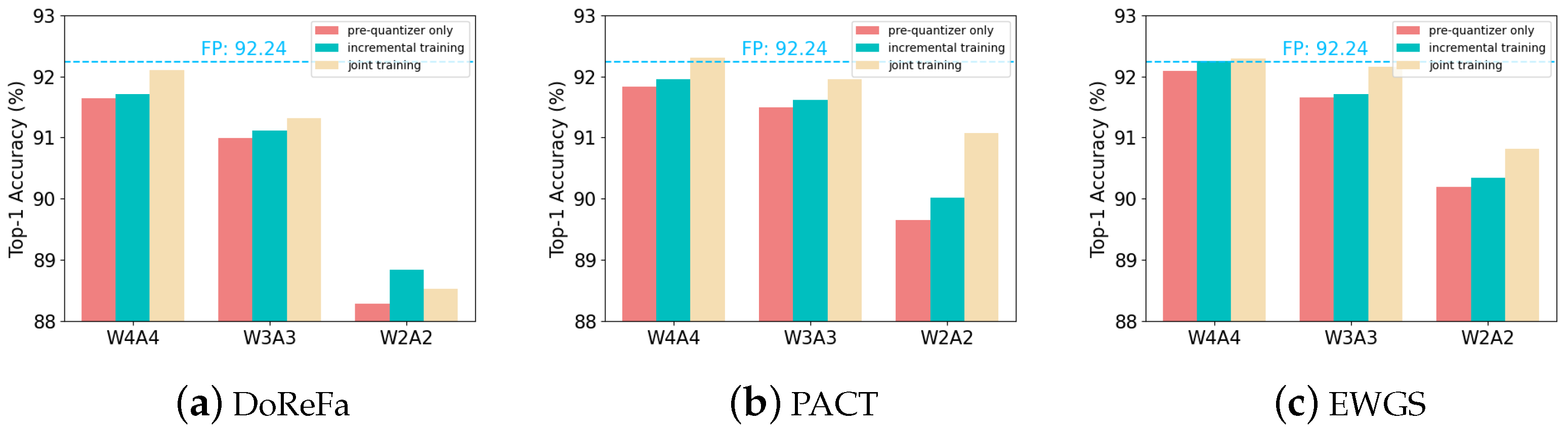
5.3.3. Evaluation of Different Training Strategies

To evaluate our proposed framework, we performed experiments under the aforementioned two training strategies. For incremental training, we treated the BWA module as an incremental component and trained it independently. The models were initialized using the parameters of the pre-quantized networks. For joint training, the BWA module was trained together with all the other parameters, and the models were initialized using the pre-trained full-precision parameters. As shown in Figure 4, three different pre-quantizers were used, including DoReFa [10], PACT [11], and EWGS [20]. We show the top-1 accuracy on CIFAR-10 [18] using the ResNet-20 architecture [1] across various bit-width settings for comparison.

The results show that (1) under both training strategies, our proposed approach resulted in considerable performance gains for all three pre-quantizers; (2) joint training generally led to more improvements in accuracy compared to incremental training; (3) with 4-bit activations and weights, our proposed method achieved higher accuracy compared to the floating-point models when using PACT and EWGS as pre-quantizers under the joint training strategy; and (4) the accuracy of the 4-bit quantized model surpassed that of the full-precision model under the incremental training strategy when using EWGS as a pre-quantizer. The experimental results verify the effectiveness of the two training strategies.

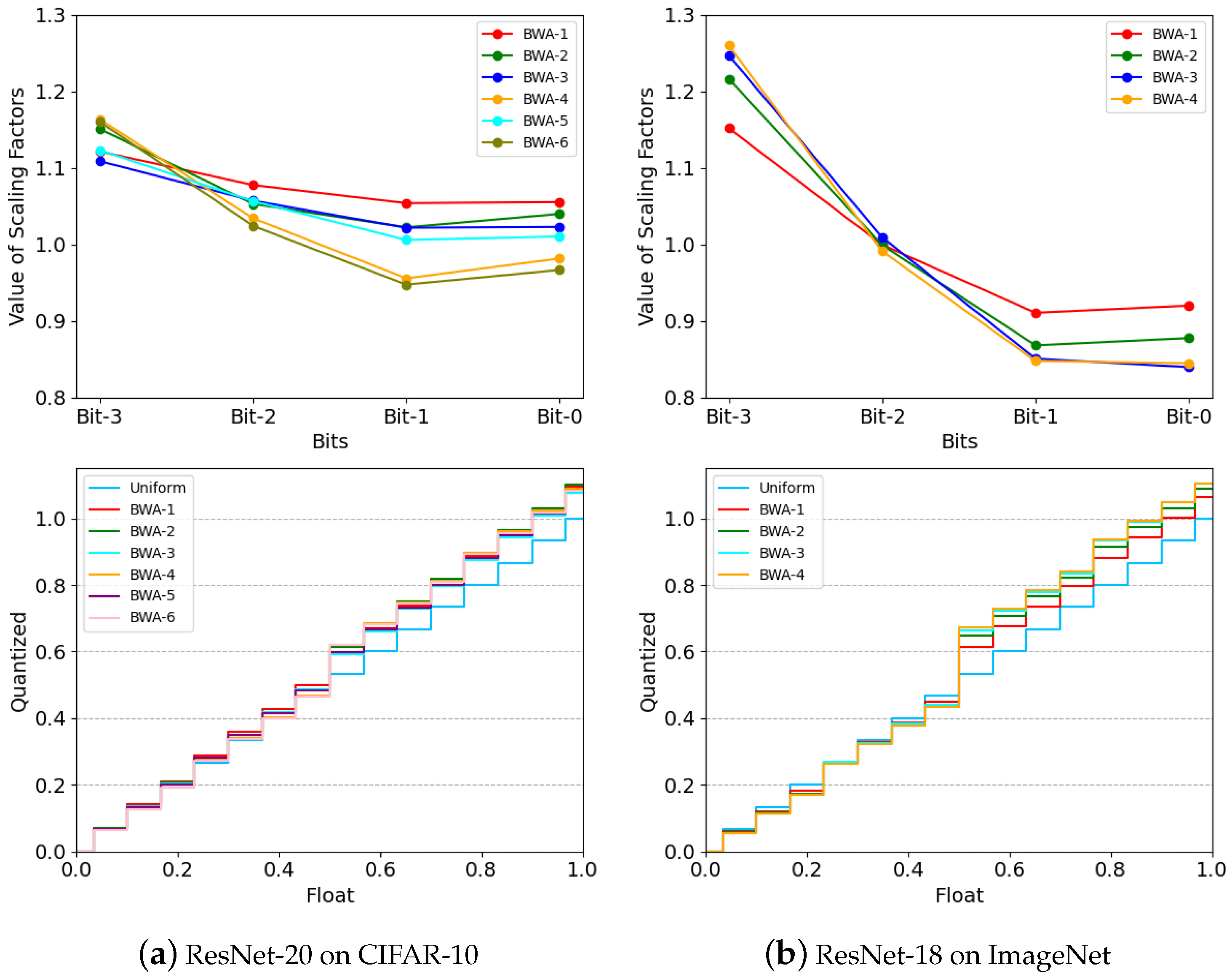
5.4. Analysis of Scaling Factors

In Figure 5, we show the values of the scaling factors and the trained quantization levels of different layers in 4-bit quantized neural networks. From the figure, we can observe that the values of the scaling factors of different BWA modules exhibit the same trend, although different BWA modules possess different scaling factors. The trend shows that the values of the scaling factors of all BWA modules actually decreased from the high end to the low end. Allocating larger scaling factors to high-end bits actually increased the relative weights of high-end bits for the quantized data, suggesting that high-end bits play a more important role compared to low-end bits, thereby contributing more to the quantized data.

We can also analyze this phenomenon from the perspective of the quantization levels. Equation (2) gives the relationship between the coefficients and quantization levels, demonstrating that different quantization levels are actually sums of different combinations of a certain set of coefficients. If the values of the coefficients change, so do the quantization levels. The lower row in Figure 5 shows the corresponding quantization levels of the trained BWA modules. We can clearly see from the figure that the trained quantization levels are non-uniformly spaced and vary from module to module. This demonstrates the ability of the BWA module to transform uniformly quantized data into a non-uniformly quantized form. In addition, it also illustrates that a simple uniform quantization scheme is sub-optimal and that the best quantization scheme varies across layers. In the BWA module, the quantization levels are automatically learned to be adaptive to different layers so better performance can be achieved. We can also observe a commonality between the trained quantization levels of BWA modules: the trained levels tend to cluster just above 0.5. This can be attributed to the highest weight of the highest-end bit, which accounts for more than half of the whole value.

5.5. Memory Efficiency and Computational Cost

5.5.1. Memory Efficiency

We present the impact of typical quantization on compressing model size and reducing memory access cost in

Table 5. Sizes and memory access costs across different models and precisions.

Model	Bit Width (W/A)	Model Size (MB)	Memory Access (MB)
ResNet-18	32/32	44.59	6985.09
	4/4	5.61	1282.73
	3/3	4.22	1079.08
	2/2	2.83	875.42
ResNet-20	32/32	1.03	157.55
	4/4	0.13	22.21
	3/3	0.10	17.38
	2/2	0.07	12.55

. Generally, model size depends on both the number of parameters it possesses and the precision used to represent these parameters. By representing the model parameters with low-precision values, the model size can be significantly compressed. Table 5 shows that the model size was compressed approximately $8\times$, $10\times$, and $15\times$ with 4-bit, 3-bit, and 2-bit quantization, respectively. Memory access cost refers to the total amount of memory reads and writes required for a single network inference and is another critical factor to consider. Table 5 demonstrates the memory access costs across the different models and representation precisions. Using four or fewer bit representations reduced the memory access cost by over $80\%$. It is worth noting that the memory access cost is a key factor affecting the energy consumption and inference speed of a model. Reducing this cost also improves energy efficiency and inference speed.

Although our approach introduces extra parameters (i.e., scaling factors ${\alpha }_i$ in BWA modules), it can still achieve nearly the same memory efficiency as typical uniform quantization.

Table 6. Number of parameters of 4-bit quantized models.

Model	Method	Params
ResNet-18	Uniform	11,689,603
	Ours	11,689,619 (+0.001%)
ResNet-20	Uniform	269,934
	Ours	269,958 (+0.089%)

shows a comparison of the number of parameters between our method and uniform quantization methods. Obviously, our approach led to only a slight increase in the number of parameters, which was negligible considering the huge number of weight parameters in neural networks. Moreover, the number of parameters introduced in our approach was proportional to the number of bits. The lower the precision used, the fewer the number of parameters introduced. Therefore, our approach achieved almost the same compression levels as those shown in Table 5.

5.5.2. Computational Cost

After quantizing both the weights and activations, a standard 32-bit convolution can be substituted with the sum of the binary convolutions, as shown in Equation (3). Bitwise operations like $and$, $xnor$, and $popcnt$ can be leveraged to compute the binary convolutions, significantly reducing computational complexity. Assume that the activations and weights are represented using M and N bits, respectively. Let k be the size of the filter kernel, $W_o$ and $H_o$ be the width and height of the output feature map, and $C_i$ and $C_o$ be the number of input and output channels. When using uniform quantization, Equation (3) involves $(2k^2{C}_i-1)MN{C}_o{H}_o{W}_o$ bitwise operations and $(2MN-1)C_o{H}_o{W}_o$ fixed-point operations. Compared to the number of bitwise operations, the number of fixed-point operations is quite minimal.

In our approach, floating-point operations are involved because of the floating-point coefficients, whose number is the same as the number of fixed-point operations in uniform quantization. Note that this incurs only minimal computational cost. Firstly, compared to bitwise operations, the number of non-bitwise operations is quite minimal. Secondly, we only insert BWA modules in the last few layers of a model. Therefore, the extra computational overhead of our model is very small. Compared to existing non-uniform quantization methods that introduce floating-point operations in all quantization layers [13,15], our approach requires 14 and 6 times fewer floating-point operations for ResNet-18 and ResNet-20, respectively.

6. Conclusions

In this study, we introduced the BWA module, which adaptively learns the best quantization scheme for each layer by simply introducing trainable scaling factors. In order to benefit from both the hardware friendliness of uniform quantization and the high performance of non-uniform quantization, we proposed a strategy to combine uniform and non-uniform quantization in a single network. The BWA module builds on the idea that quantization levels can be optimized by adjusting the weight of each bit. Moreover, the module can be integrated into various existing quantization methods to improve model performance. Two different training algorithms were used to train the proposed approach. Different configurations of the proposed approach were explored to verify the effectiveness of our approach. Numerous experiments conducted on two common datasets showed that our quantized models exhibited state-of-the-art performance across various bit-width settings.

References

1. He, K.; Zhang, X.; Ren, S.; Sun, J. Deep Residual Learning for Image Recognition. In Proceedings of the IEEE/CVF Conference on Computer Vision and Pattern Recognition, Las Vegas, NV, USA, 27–30 June 2016; pp. 770–778. [Google Scholar]
2. He, K.; Zhang, X.; Ren, S.; Sun, J. Identity mappings in deep residual networks. In Proceedings of the European Conference on Computer Vision, Amsterdam, The Netherlands, 11–14 October 2016; pp. 630–645. [Google Scholar]
3. Condés, I.; Fernández-Conde, J.; Perdices, E.; Cañas, J.M. Robust Person Identification and Following in a Mobile Robot Based on Deep Learning and Optical Tracking. Electronics 2023, 12, 4424. [Google Scholar] [CrossRef]
4. Zhang, R.; Zhu, Z.; Li, L.; Bai, Y.; Shi, J. BFE-Net: Object Detection with Bidirectional Feature Enhancement. Electronics 2023, 12, 4531. [Google Scholar] [CrossRef]
5. Liang, C.; Yang, J.; Du, R.; Hu, W.; Tie, Y. Non-Uniform Motion Aggregation with Graph Convolutional Networks for Skeleton-Based Human Action Recognition. Electronics 2023, 12, 4466. [Google Scholar] [CrossRef]
6. Krizhevsky, A.; Sutskever, I.; Hinton, G.E. ImageNet Classification with Deep Convolutional Neural Networks. In Proceedings of the 25th International Conference on Neural Information Processing Systems, Lake Tahoe, NV, USA, 3–6 December 2012; Volume 1, pp. 1097–1105. [Google Scholar]
7. Iandola, F.N.; Han, S.; Moskewicz, M.W.; Ashraf, K.; Dally, W.J.; Keutzer, K. SqueezeNet: AlexNet-level accuracy with 50x fewer parameters and< 0.5 MB model size. In Proceedings of the 4th International Conference on Learning Representations, San Juan, PR, USA, 2–4 May 2016. [Google Scholar]
8. Park, S.; Lee, J.; Mo, S.; Shin, J. Lookahead: A far-sighted alternative of magnitude-based pruning. In Proceedings of the 8th International Conference on Learning Representations, Addis Ababa, Ethiopia, 26–30 April 2020. [Google Scholar]
9. Polino, A.; Pascanu, R.; Alistarh, D. Model compression via distillation and quantization. In Proceedings of the 6th International Conference on Learning Representations, Vancouver, BC, Canada, 30 April–3 May 2018. [Google Scholar]
10. Zhou, S.; Wu, Y.; Ni, Z.; Zhou, X.; Wen, H.; Zou, Y. Dorefa-net: Training low bitwidth convolutional neural networks with low bitwidth gradients. arXiv 2016, arXiv:1606.06160. [Google Scholar]
11. Choi, J.; Wang, Z.; Venkataramani, S.; Chuang, P.I.J.; Srinivasan, V.; Gopalakrishnan, K. Pact: Parameterized clipping activation for quantized neural networks. In Proceedings of the 6th International Conference on Learning Representations, Vancouver, BC, Canada, 30 April–3 May 2018. [Google Scholar]
12. Gong, R.; Liu, X.; Jiang, S.; Li, T.; Hu, P.; Lin, J.; Yu, F.; Yan, J. Differentiable soft quantization: Bridging full-precision and low-bit neural networks. In Proceedings of the IEEE/CVF International Conference on Computer Vision, Seoul, Republic of Korea, 27 October–2 November 2019; pp. 4852–4861. [Google Scholar]
13. Zhang, D.; Yang, J.; Ye, D.; Hua, G. Lq-nets: Learned quantization for highly accurate and compact deep neural networks. In Proceedings of the European Conference on Computer Vision, Munich, Germany, 8–14 September 2018; pp. 365–382. [Google Scholar]
14. Lin, X.; Zhao, C.; Pan, W. Towards accurate binary convolutional neural network. In Proceedings of the 31st Conference on Neural Information Processing Systems, Long Beach, CA, USA, 4–9 December 2017; Volume 30. [Google Scholar]
15. Qu, Z.; Zhou, Z.; Cheng, Y.; Thiele, L. Adaptive loss-aware quantization for multi-bit networks. In Proceedings of the IEEE/CVF Conference on Computer Vision and Pattern Recognition, Seattle, WA, USA, 13–19 June 2020; pp. 7988–7997. [Google Scholar]
16. Jung, S.; Son, C.; Lee, S.; Son, J.; Han, J.J.; Kwak, Y.; Hwang, S.J.; Choi, C. Learning to quantize deep networks by optimizing quantization intervals with task loss. In Proceedings of the IEEE/CVF Conference on Computer Vision and Pattern Recognition, Long Beach, CA, USA, 15–20 June 2019; pp. 4350–4359. [Google Scholar]
17. Deng, J.; Dong, W.; Socher, R.; Li, L.J.; Li, K.; Li, F.-F. Imagenet: A large-scale hierarchical image database. In Proceedings of the IEEE/CVF Conference on Computer Vision and Pattern Recognition, Miami, FL, USA, 20–25 June 2009. [Google Scholar]
18. Krizhevsky, A.; Hinton, G. Learning Multiple Layers of Features from Tiny Images. 2009. Available online: https://www.cs.toronto.edu/~kriz/learning-features-2009-TR.pdf (accessed on 10 April 2023).
19. Dong, Z.; Yao, Z.; Arfeen, D.; Gholami, A.; Mahoney, M.W.; Keutzer, K. Hawq-v2: Hessian aware trace-weighted quantization of neural networks. In Proceedings of the Conference on Neural Information Processing Systems, Virtual Event, 6–12 December 2020; Volume 33, pp. 18518–18529. [Google Scholar]
20. Lee, J.; Kim, D.; Ham, B. Network quantization with element-wise gradient scaling. In Proceedings of the IEEE/CVF Conference on Computer Vision and Pattern Recognition, Nashville, TN, USA, 20–25 June 2021; pp. 6448–6457. [Google Scholar]
21. Miyashita, D.; Lee, E.H.; Murmann, B. Convolutional neural networks using logarithmic data representation. arXiv 2016, arXiv:1603.01025. [Google Scholar]
22. Xu, J.; Huan, Y.; Jin, Y.; Chu, H.; Zheng, L.R.; Zou, Z. Base-reconfigurable segmented logarithmic quantization and hardware design for deep neural networks. J. Signal Process. Syst. 2020, 92, 1263–1276. [Google Scholar] [CrossRef]
23. Zhou, A.; Yao, A.; Guo, Y.; Xu, L.; Chen, Y. Incremental network quantization: Towards lossless cnns with low-precision weights. In Proceedings of the 5th International Conference on Learning Representations, Toulon, France, 24–26 April 2017. [Google Scholar]
24. Lee, E.H.; Miyashita, D.; Chai, E.; Murmann, B.; Wong, S.S. Lognet: Energy-efficient neural networks using logarithmic computation. In Proceedings of the IEEE International Conference on Acoustics, Speech and Signal Processing, New Orleans, LA, USA, 5–9 March 2017; pp. 5900–5904. [Google Scholar]
25. Lee, S.; Sim, H.; Choi, J.; Lee, J. Successive log quantization for cost-efficient neural networks using stochastic computing. In Proceedings of the 56th ACM/IEEE Design Automation Conference (DAC), Las Vegas, NV, USA, 2–6 June 2019; pp. 1–6. [Google Scholar]
26. Xu, C.; Yao, J.; Lin, Z.; Ou, W.; Cao, Y.; Wang, Z.; Zha, H. Alternating multi-bit quantization for recurrent neural networks. In Proceedings of the 6th International Conference on Learning Representations, Vancouver, BC, Canada, 30 April–3 May 2018. [Google Scholar]
27. Li, Z.; Ni, B.; Zhang, W.; Yang, X.; Gao, W. Performance guaranteed network acceleration via high-order residual quantization. In Proceedings of the IEEE/CVF International Conference on Computer Vision, Venice, Italy, 22–29 October 2017; pp. 2584–2592. [Google Scholar]
28. Paszke, A.; Gross, S.; Chintala, S.; Chanan, G.; Yang, E.; DeVito, Z.; Lin, Z.; Desmaison, A.; Antiga, L.; Lerer, A. Automatic differentiation in pytorch. In Proceedings of the 31st Conference on Neural Information Processing Systems, Long Beach, CA, USA, 4–9 December 2017. [Google Scholar]
29. Loshchilov, I.; Hutter, F. Sgdr: Stochastic gradient descent with warm restarts. In Proceedings of the 5th International Conference on Learning Representations, Toulon, France, 24–26 April 2017. [Google Scholar]
30. Yang, H.; Duan, L.; Chen, Y.; Li, H. BSQ: Exploring bit-level sparsity for mixed-precision neural network quantization. In Proceedings of the 9th International Conference on Learning Representations, Virtual Event, 3–7 May 2021. [Google Scholar]
31. Yamamoto, K. Learnable companding quantization for accurate low-bit neural networks. In Proceedings of the IEEE/CVF Conference on Computer Vision and Pattern Recognition, Nashville, TN, USA, 20–25 June 2021; pp. 5029–5038. [Google Scholar]
32. Wang, L.; Dong, X.; Wang, Y.; Liu, L.; An, W.; Guo, Y.K. Learnable Lookup Table for Neural Network Quantization. In Proceedings of the IEEE/CVF Conference on Computer Vision and Pattern Recognition, New Orleans, LA, USA, 18–24 June 2022; pp. 12413–12423. [Google Scholar]
33. Lin, S.T.; Li, Z.; Cheng, Y.H.; Kuo, H.W.; Lu, C.C.; Tang, K.T. LG-LSQ: Learned Gradient Linear Symmetric Quantization. arXiv 2022, arXiv:2202.09009. [Google Scholar]
34. Xu, K.; Lee, A.H.X.; Zhao, Z.; Wang, Z.; Wu, M.; Lin, W. MetaGrad: Adaptive Gradient Quantization with Hypernetworks. arXiv 2023, arXiv:2303.02347. [Google Scholar]
35. Liu, H.; Elkerdawy, S.; Ray, N.; Elhoushi, M. Layer importance estimation with imprinting for neural network quantization. In Proceedings of the IEEE/CVF Conference on Computer Vision and Pattern Recognition, Nashville, TN, USA, 20–25 June 2021; pp. 2408–2417. [Google Scholar]
36. Li, Y.; Dong, X.; Wang, W. Additive powers-of-two quantization: An efficient non-uniform discretization for neural networks. In Proceedings of the 8th International Conference on Learning Representations, Addis Ababa, Ethiopia, 26–30 April 2020. [Google Scholar]
37. Esser, S.K.; McKinstry, J.L.; Bablani, D.; Appuswamy, R.; Modha, D.S. Learned step size quantization. In Proceedings of the 8th International Conference on Learning Representations, Addis Ababa, Ethiopia, 26–30 April 2020. [Google Scholar]
38. Bhalgat, Y.; Lee, J.; Nagel, M.; Blankevoort, T.; Kwak, N. Lsq+: Improving low-bit quantization through learnable offsets and better initialization. In Proceedings of the IEEE/CVF Conference on Computer Vision and Pattern Recognition Workshops, Seattle, WA, USA, 14–19 June 2020; pp. 696–697. [Google Scholar]
39. Kim, D.; Lee, J.; Ham, B. Distance-aware Quantization. In Proceedings of the IEEE/CVF International Conference on Computer Vision, Montreal, BC, Canada, 11–17 October 2021; pp. 5271–5280. [Google Scholar]
40. Tang, C.; Ouyang, K.; Wang, Z.; Zhu, Y.; Wang, Y.; Ji, W.Z.; Zhu, W. Mixed-Precision Neural Network Quantization via Learned Layer-wise Importance. In Proceedings of the European Conference on Computer Vision, Tel Aviv, Israel, 23–27 October 2022; pp. 259–275. [Google Scholar]
41. Tang, C.; Ouyang, K.; Chai, Z.; Bai, Y.; Meng, Y.; Wang, Z.; Zhu, W. SEAM: Searching Transferable Mixed-Precision Quantization Policy through Large Margin Regularization. In Proceedings of the 31st ACM International Conference on Multimedia, Vancouver, BC, Canada, 7–10 June 2023. [Google Scholar]
Figure 1. An illustration of the underlying logic of the proposed BWA module. The BWA module transforms uniformly spaced quantization levels into non-uniformly spaced forms by adjusting the weight of each bit using scaling factors.
Electronics 12 05043 g001
Figure 2. An illustration of a neural network with our activation quantization blocks. A quantization block is expanded to show the details. Each quantization block is composed of a pre-quantizer and a BWA module. The BWA module is indicated by dashed lines because it is optionally inserted into each quantization block.
Electronics 12 05043 g002
Figure 3. The activation distributions of several layers of ResNet-20.
Electronics 12 05043 g003
Figure 4. Validation accuracy comparison: the top-1 accuracy of ResNet-20 on CIFAR-10 using multiple pre-quantizers under different training strategies.
Electronics 12 05043 g004
Figure 5. Visualization of the scaling factors (upper) and trained quantization levels (lower) of different layers with BWA modules in 4-bit quantized neural networks. BWA-i denotes the i-th BWA module inserted in the network.
Electronics 12 05043 g005