
Aperture-Level Simultaneous Transmit and Receive Simplified Structure Based on Hybrid Beamforming of Switching Network


Abstract
:1. Introduction
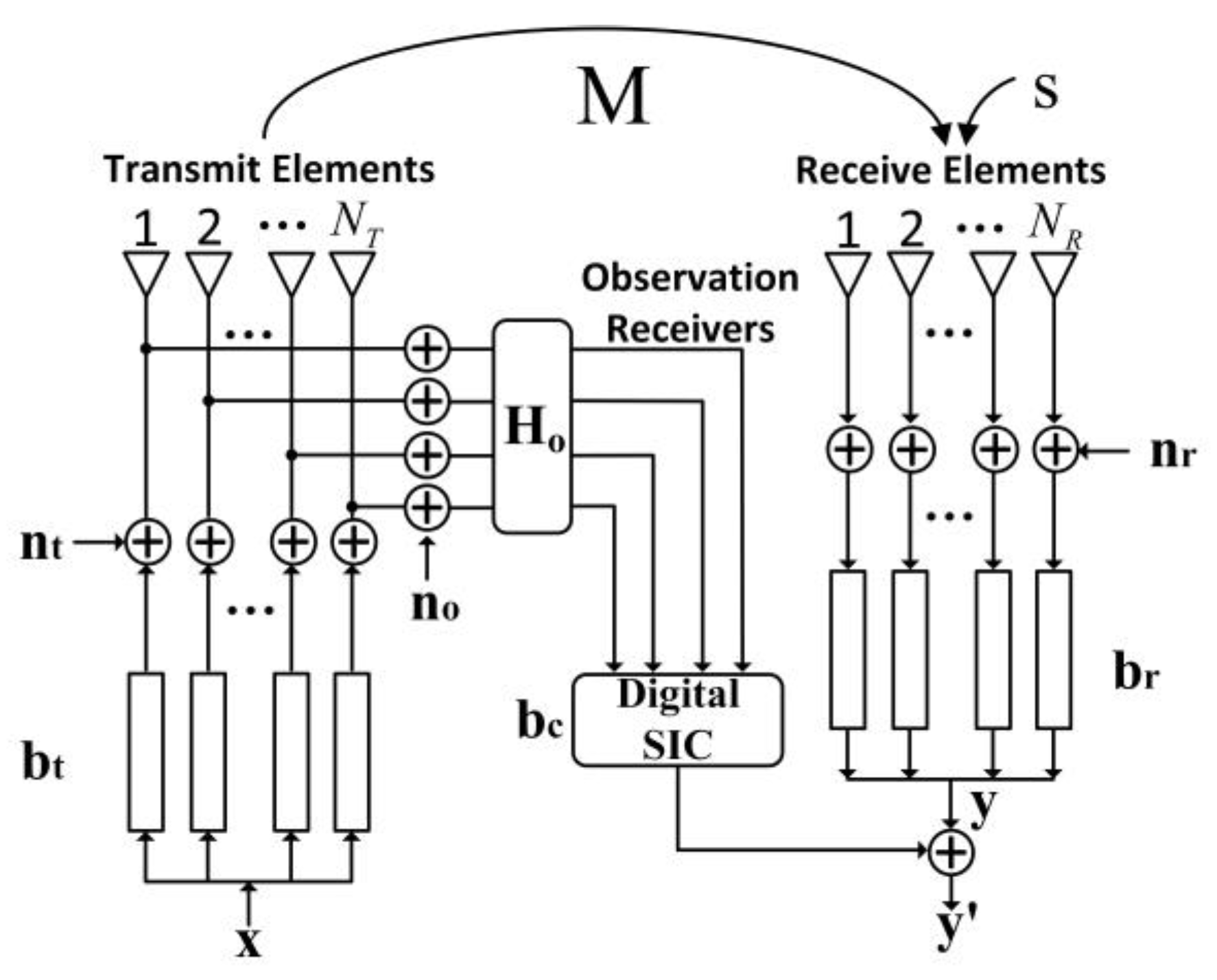
2. System Model
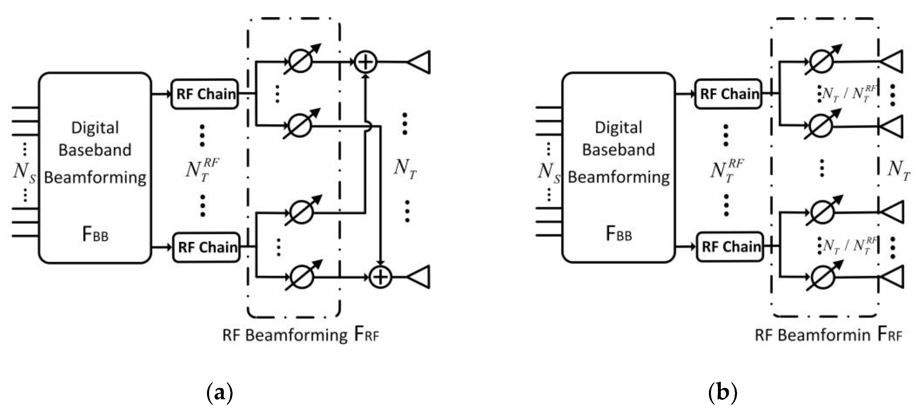
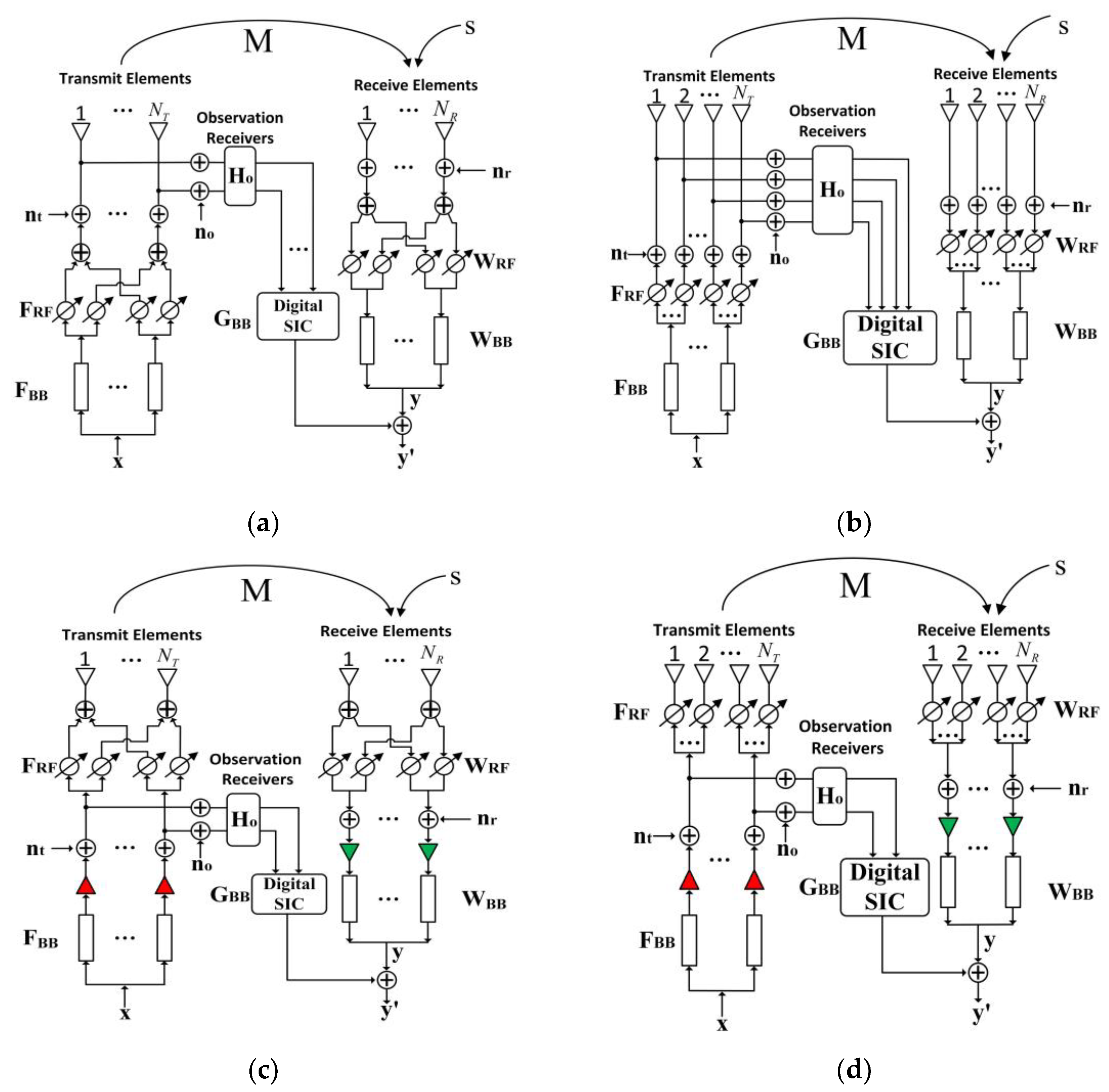
2.1. Aperture-Level Simultaneous Transmit and Receive Simplified Structure Based on Hybrid Beamforming (HBF-ALSTAR)
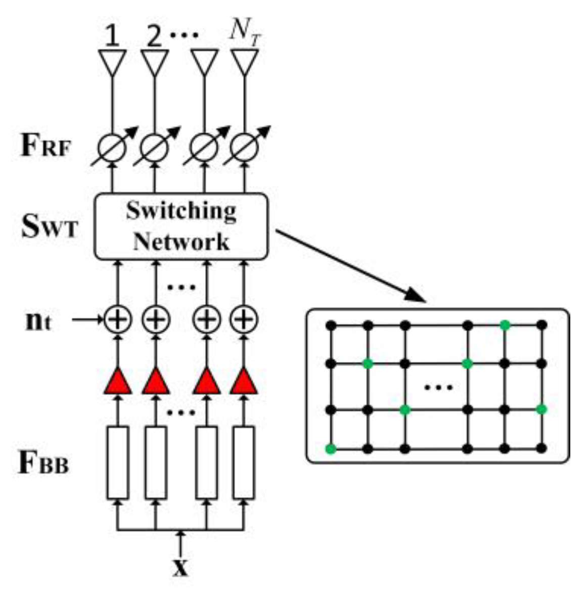
2.2. Aperture-Level Simultaneous Transmit and Receive Simplified Structure Based on Hybrid Beamforming of Switching Network (HBF-SN-ALSTAR)
3. Simulation Experiment
3.1. Channel Parameter
3.2. Experimental Parameters
4. Conclusions
Author Contributions
Funding
Data Availability Statement
Conflicts of Interest
References
- Bojja Venkatakrishnan, S.; Alwan, E.A.; Volakis, J.L. Wideband RF Self-Interference Cancellation Circuit for Phased Array Simultaneous Transmit and Receive Systems. IEEE Access 2018, 6, 3425–3432. [Google Scholar] [CrossRef]
- Gheorma, I.L.; Gopalakrishnan, G.K. RF Photonic Techniques for Same Frequency Simultaneous Duplex Antenna Operation. IEEE Photon. Technol. Lett. 2007, 19, 1014–1016. [Google Scholar] [CrossRef]
- Ranjbar Nikkhah, M.; Wu, J.; Luyen, H.; Behdad, N. A Concurrently Dual-Polarized, Simultaneous Transmit and Receive (STAR) Antenna. IEEE Trans. Antennas Propagat. 2020, 68, 5935–5944. [Google Scholar] [CrossRef]
- Doane, J.P.; Kolodziej, K.E.; Perry, B.T. Simultaneous transmit and receive with digital phased arrays. In Proceedings of the 2016 IEEE International Symposium on Phased Array Systems and Technology (PAST), Waltham, MA, USA, 18–21 October 2016. [Google Scholar]
- Cummings, I.T.; Doane, J.P.; Schulz, T.J.; Havens, T.C. Aperture-Level Simultaneous Transmit and Receive with Digital Phased Arrays. IEEE Trans. Signal Process. 2020, 68, 1243–1258. [Google Scholar] [CrossRef]
- Chen, Z.; Zhang, X.; Wang, S.; Xu, Y.; Xiong, J.; Wang, X. Enabling Practical Large-Scale MIMO in WLANs With Hybrid Beamforming. IEEE/ACM Trans. Netw. 2021, 29, 1605–1619. [Google Scholar] [CrossRef]
- Ayach, O.E.; Rajagopal, S.; Abu-Surra, S.; Pi, Z.; Heath, R.W. Spatially Sparse Precoding in Millimeter Wave MIMO Systems. IEEE Trans. Wireless Commun. 2014, 13, 1499–1513. [Google Scholar] [CrossRef] [Green Version]
- Zhang, X.; Molisch, A.F.; Kung, S. Variable-phase-shift-based RF-baseband codesign for MIMO antenna selection. IEEE Trans. Signal Process. 2005, 53, 4091–4103. [Google Scholar] [CrossRef]
- Heath, R.W.; González-Prelcic, N.; Rangan, S.; Roh, W.; Sayeed, A.M. An Overview of Signal Processing Techniques for Millimeter Wave MIMO Systems. IEEE J. Sel. Top. Sign. Proces. 2016, 10, 436–453. [Google Scholar] [CrossRef]
- Li, A.; Masouros, C. Hybrid Analog-Digital Millimeter-Wave MU-MIMO Transmission with Virtual Path Selection. IEEE Commun. Lett. 2017, 21, 438–441. [Google Scholar] [CrossRef] [Green Version]
- Lee, Y.; Wang, C.; Huang, Y. A Hybrid RF/Baseband Precoding Processor Based on Parallel-Index-Selection Matrix-Inversion-Bypass Simultaneous Orthogonal Matching Pursuit for Millimeter Wave MIMO Systems. IEEE Trans. Signal Process. 2015, 63, 305–317. [Google Scholar] [CrossRef]
- Ortega, A.J. Transforming the fully connected structures of hybrid precoders into dynamic partially connected structures. In Proceedings of the 2021 28th International Conference on Telecommunications (ICT), London, UK, 1–3 June 2021. [Google Scholar]
- Li, N.; Wei, Z.; Yang, H.; Zhang, X.; Yang, D. Hybrid Precoding for mmWave Massive MIMO Systems with Partially Connected Structure. IEEE Access 2017, 5, 15142–15151. [Google Scholar] [CrossRef]
- Pang, L.; Wu, W.; Zhang, Y.; Gong, W.; Shang, M.; Chen, Y.; Wang, A. Iterative Hybrid Precoding and Combining for Partially Connected Massive MIMO mmWave Systems. In Proceedings of the 2020 IEEE 92nd Vehicular Technology Conference (VTC2020-Fall), Victoria, BC, Canada, 18 November–16 December 2020. [Google Scholar]
- Yu, X.; Shen, J.-C.; Zhang, J.; Letaief, K.B. Alternating Minimization Algorithms for Hybrid Precoding in Millimeter Wave MIMO Systems. IEEE J. Sel. Top. Sign. Proces. 2016, 10, 485–500. [Google Scholar] [CrossRef] [Green Version]
- Yi, H.; Wei, X.; Tang, Y. Hybrid Precoding Based on a Switching Network in Millimeter Wave MIMO Systems. Electronics 2022, 11, 2541. [Google Scholar] [CrossRef]
- Sohrabi, F.; Yu, W. Hybrid Digital and Analog Beamforming Design for Large-Scale Antenna Arrays. IEEE J. Select. Top. Sign. Proces. 2016, 10, 501–513. [Google Scholar] [CrossRef]
- Kasai, H. Fast Optimization Algorithm on Complex Oblique Manifold for Hybrid Precoding in Millimeter Wave MIMO Systems. In Proceedings of the 2018 IEEE Global Conference on Signal and Information Processing (GlobalSIP), Anaheim, CA, USA, 26–29 November 2018. [Google Scholar]


| Acronym | Definition |
|---|---|
| STAR | Simultaneous Transmit and Receive |
| FD-ALSTAR | Full Digital Aperture-Level Simultaneous Transmit and Receive |
| NRF | Number of RF Links |
| HBF-SN-ALSTAR | Aperture-Level Simultaneous Transmit and Receive Simplified Structure Based on Hybrid Beamforming of Switching Network |
| EII | Effective Isotropic Isolation |
| FDD | Frequency Division Duplex |
| TDD | Time Division Duplex |
| SIC | Self-Interference Cancellation |
| ADC/DAC | Analog-to-Digital Converter /Digital-to-Analog Converter |
| FC | Fully Connected |
| PC | Partially Connected |
| ZF | Zero Forcing Algorithm |
| OMP | Orthogonal Matching Pursuit Algorithm |
| MO-AltMin | Manifold Optimization Based Hybrid Precoding for the Fully connected |
| SDR-AltMin | Semidefinite Relaxation Based Hybrid Precoding for the Partially connected |
| HBF-ALSTAR | Aperture-Level Simultaneous Transmit and Receive Simplified Structure Based on Hybrid Beamforming |
| HBF-FC-ALSTAR-AO | Aperture-Level Simultaneous Transmit and Receive Simplified Structure Based on Antenna End Observation of Fully Connected Hybrid Beamforming |
| HBF-PC-ALSTAR-AO | Aperture-Level Simultaneous Transmit and Receive Simplified Structure Based on Antenna End Observation of Partially Connected Hybrid Beamforming |
| HBF-FC-ALSTAR-RFO | Aperture-Level Simultaneous Transmit and Receive Simplified Structure Based on RF Links Observation of Fully Connected Hybrid Beamforming |
| HBF-PC-ALSTAR-RFO | Aperture-Level Simultaneous Transmit and Receive Simplified Structure Based on RF Links Observation of Partially Connected Hybrid Beamforming |
| HBF-SN-ALSTAR-AO | Aperture-Level Simultaneous Transmit and Receive Simplified Structure Based on antenna end observation of Hybrid Beamforming of Switching Network |
| HBF-SN-ALSTAR-RFO | Aperture-Level Simultaneous Transmit and Receive Simplified Structure Based on RF links observation of Hybrid Beamforming of Switching Network |
| EIRP | Effective Isotropic Radiated Power |
| EIS | Effective Isotropic Sensitivity |
| HBF-SN-H-ALSTAR | Aperture-Level Simultaneous Transmit and Receive Simplified Structure Based on Hybrid Beamforming of Switching Network of Statistical Dynamic Grouping |
| HBF-SN-A-ALSTAR | Aperture-Level Simultaneous Transmit and Receive Simplified Structure Based on Hybrid Beamforming of Switching Network of Average Dynamic Grouping |
| AOD | Angles of Departure |
| AOA | Angles of Arrival |
| USPA | Uniform Square Array |
| Electronic Device | HBF-FC-ALSTAR-RFO | HBF-PC-ALSTAR-RFO | HBF-SN-ALSTAR-A-RFO |
|---|---|---|---|
| DAC | 24 | 24 | 24 |
| ADC | 24 | 24 | 24 |
| PA | 24 | 24 | 24 |
| Frequency Mixer | 144 | 144 | 144 |
| Phase Shifter | 3456 | 144 | 144 |
| Switching Network | 0 | 0 | 1 (144 × 24) |
| Power Combiner | 144 (144 to 1) | 0 | 0 |
| Power Divider | 24 (1 to 144) | 24 (1 to 6) | 24 (1 to 6) |
Disclaimer/Publisher’s Note: The statements, opinions and data contained in all publications are solely those of the individual author(s) and contributor(s) and not of MDPI and/or the editor(s). MDPI and/or the editor(s) disclaim responsibility for any injury to people or property resulting from any ideas, methods, instructions or products referred to in the content. |
© 2023 by the authors. Licensee MDPI, Basel, Switzerland. This article is an open access article distributed under the terms and conditions of the Creative Commons Attribution (CC BY) license (https://creativecommons.org/licenses/by/4.0/).
Share and Cite
Yi, H.; Wei, X.; Lin, T.; Tang, Y.; Xie, M.; Hu, D. Aperture-Level Simultaneous Transmit and Receive Simplified Structure Based on Hybrid Beamforming of Switching Network. Electronics 2023, 12, 602. https://doi.org/10.3390/electronics12030602
Yi H, Wei X, Lin T, Tang Y, Xie M, Hu D. Aperture-Level Simultaneous Transmit and Receive Simplified Structure Based on Hybrid Beamforming of Switching Network. Electronics. 2023; 12(3):602. https://doi.org/10.3390/electronics12030602
Chicago/Turabian StyleYi, Hongbin, Xizhang Wei, Tairan Lin, Yanqun Tang, Mingcong Xie, and Dujuan Hu. 2023. "Aperture-Level Simultaneous Transmit and Receive Simplified Structure Based on Hybrid Beamforming of Switching Network" Electronics 12, no. 3: 602. https://doi.org/10.3390/electronics12030602