Wideband Direction-of-Arrival Estimation Based on Hierarchical Sparse Bayesian Learning for Signals with the Same or Different Frequency Bands

Abstract

Wideband sparse Bayesian learning (WSBL) based on joint sparsity achieves high direction-of-arrival (DOA) estimation precision when the signals share the same frequency band. However, when the signal frequency bands are non-overlapped or partially overlapped, i.e., the frequency bands are different, the performance of the method degrades due to the improper prior on signal. This paper aims at extending the WSBL to a more general version, which is also suitable for the cases where the signal frequency bands are non-overlapped or partially overlapped. Given that the signals are sparsely distributed in the space, the signal matrix whose column is composed of the signal in each frequency bin is row-sparse. Moreover, the signal vectors in some frequency bins have different sparse supports when the signals occupy the different frequency bands. Therefore, a hierarchical sparse prior is assigned to the signal matrix, where a set of hyperparameters are used to ensure the row-sparsity and the other set are used to adjust the signal sparsity in each frequency bin. The DOAs are finally estimated in the Bayesian framework. The simulation results verify that the proposed method achieves good performance on estimation precision in both the same and different frequency band scenarios.

1. Introduction

Direction-of-arrival (DOA) estimation is an important research subject in sonar array signal processing [1,2]. Recently, sparse reconstruction methods [3,4,5,6,7,8,9] have attracted considerable attention. In comparison with traditional high-resolution methods [10,11,12], they can be applied in the lower signal-to-noise ratio (SNR) cases [3]. This kind of method divides the space into the discretized grid points and the steering vectors of the grid points form the dictionary matrix. Then, a linear combination among these bases is selected to fit the received data. These methods can be roughly classified into two categories: l_p-norm-based method [3,4,5] and sparse Bayesian learning (SBL) method [13,14]. The l_p-norm-based method needs to well tune a regularization parameter to control the tradeoff between the sparsity levels and the data fitting error. Different value of this parameter leads to different estimates [3]. However, the optimal parameter is hard obtained [15,16]. In contrast, the SBL method can automatically tune the hyperparameters from the received data. Therefore, it can be easily applied in practical signal processing.

Nowadays, wideband signal processing is widely used in many applications [17]. A direct way to achieve wideband DOA estimation is to transform the data into frequency domain through Fourier transformation. As such, the signal in each frequency bin is narrowband signal. The narrowband sparse reconstruction methods can be directly applied in each frequency bin, and the estimation results are then summed to obtain the wideband spatial spectrum, which is an independent processing (IP) among frequency bins [5]. The estimation precision of incoherent processing is seriously affected by a large estimation bias in a frequency bin. Hence, it needs high SNR to maintain good performance [18]. To coherently process the data in each frequency bin, the focusing matrix [18,19,20] is used to transform the signal subspace in each frequency bin into the focusing frequency bin. In this manner, the wideband DOA estimation problem is transformed into the narrowband one at the focusing frequency. However, the DOA information is needed as a prior in this kind of method to design the focusing matrix, which is known as the focusing angles. A large bias between the focusing angles and true DOAs leads to inaccurate DOA estimates [21].

To avoid above problems, He et al. [22] proposed a wideband sparse spectrum fitting (W-SpSF) method. It expresses the received data in all frequency bins into a matrix, and the signal vectors in all frequency bins are also written into a matrix, which forms a signal matrix. Clearly, this matrix is a row-sparse matrix since the signal vectors are sparse. As such, this method uses l_2,1-norm to the signal matrix as the sparse penalty term to control the row-sparsity, thus jointly processing the data in all frequency bins. However, the W-SpSF is a kind of l_p-norm-based method. As mentioned above, the optimal regularization parameter is hard selected [15,16]. Moreover, the method suffers from low computational efficiency since the dimension of the dictionary matrix increases by expressing all frequency bins into a matrix. Das et al. [23] proposed the wideband SBL (WSBL) method. This method assigns the same prior to the signal vectors in all frequency bins, where the common hyperparameters control the signal sparsity in each frequency bin. In this manner, the sparsity of the estimate is determined by all frequency bins jointly, and the estimated signal matrix must be a row-sparse matrix. This thought is also used in other works [24,25,26]. However, this kind of method only considers the condition where the signals occupy the same frequency band and the signal vectors share the same sparse support in all frequency bins. It does not consider the condition where the signals from different angles have different frequency bands and the sparse supports in different frequency bins are not totally the same. Under such conditions, the performances of these methods are obviously degraded.

This paper extends the WSBL to a more general version, which is also suitable for the case where the signal frequency bands are different. As mentioned above, the signal matrix is a row-sparse matrix. The proposed method firstly assigns a set of hyperparameters to control the row-sparsity of the signal matrix. Then, considering that the sparse supports of the signal vectors in different frequency bins are not totally the same if the signal frequency bands are different, other hyperparameters are used to adjust the signal sparsity in each frequency bin. In this manner, a hierarchical sparse prior is assigned to the signal matrix and a Bayesian probabilistic model is established. The variational Bayesian inference (VBI) [27,28] is used to estimate the hyperparameters in this model, thus achieving wideband DOA estimation. The proposed method can be regarded as a combination of the IP and joint processing (JP). Numerical simulation results verify that the proposed method achieves high DOA estimation precision under the conditions where the signal frequency bands are non-overlapped, partially overlapped and common.

The following notations are used throughout this paper: ${(·)}^H$, ${(·)}^T$ and ${(·)}^{*}$ represent the conjugate transpose, transpose and conjugate, respectively; $tr\{·\}$ and $\circ$ denote the trace operator and Hadamard product, respectively; ${\Vert ·\Vert }_2$ and $|·|$ denote the l₂-norm and modulus, respectively; $diag(\mathbf{x})$ is a diagonal matrix with entries in vector x being its diagonal elements; $diag(\mathbf{X})$ represents a vector composed of the diagonal entries of matrix X. ${\mathbf{X}}^{-1}$ means the inverse of the matrix X; $round(x)$ rounds x to the nearest integer; ${\mathbf{I}}_M$ is an $M\times M$ identity matrix; $1_{Q\times 1}$ and $0_Q$ are $Q\times 1$ vectors whose entries are all 1 and 0, respectively.

2. Signal Model Establishment

Assume that K signals impinge on an M-element array from $\mathsf{\theta }={[{\theta }_1,\dots ,{\theta }_K]}^T$. The sampling frequency is $f_s$. The received data are divided into N segments and are transformed into frequency domain in each segment through $\tilde{L}$-point discrete Fourier transformation (DFT). In this manner, the frequency resolution is $\mathrm{\Delta }f=f_s/\tilde{L}$. Record the analysis frequency range as $[f^L, f^H]$. The array output model $x_l(n)\in {ℂ}^{M\times 1}$ in the lth sub-band is established as

$$x_l\left(n\right)=A_l\left(\mathsf{\theta }\right)s_l\left(n\right)+e_l\left(n\right), n=1,\dots ,N, l=1,\dots ,L$$

(1)

where the center frequency of the lth sub-band is $f_l=round(f^L/\mathrm{\Delta }f+l-1)\mathrm{\Delta }f$, $L=round[(f^H-f^L)/\mathrm{\Delta }f]+1$, $x_l(n)\in {ℂ}^{M\times 1}$, $s_l(n)\in {ℂ}^{K\times 1}$, and $e_l(n)\in {ℂ}^{M\times 1}$ denote the DFT coefficients of the received data, the signals, and the additive noise at the nth segment, respectively. $A_l(\mathsf{\theta })=[a_l({\theta }_1),\dots ,a_l({\theta }_K)]$, where $a_l(\theta )$ is the steering vector from the direction $\theta$. Clearly, $s_{lk}(n)=0$ if the frequency $f_l$ is not contained in the signal at ${\theta }_k$, where $s_{lk}(n)$ is the kth entry of $s_l(n)$.

With the whole space divided into the discretized grid $\stackrel{⌢}{\mathsf{\theta }}={[{\stackrel{⌢}{\theta }}_1,\dots ,{\stackrel{⌢}{\theta }}_Q]}^T$, Equation (1) can be rewritten as

$$x_l\left(n\right)=A_l\left({\displaystyle \stackrel{⌢}{\mathsf{\theta }}}\right){\stackrel{⌢}{s}}_l\left(n\right)+e_l\left(n\right), n=1,\dots ,N, l=1,\dots ,L,$$

(2)

where $A_l(\stackrel{⌢}{\mathsf{\theta }})=[a_l({\stackrel{⌢}{\theta }}_1),\dots ,a_l({\stackrel{⌢}{\theta }}_Q)]$, and ${\stackrel{⌢}{s}}_l(n)\in {ℂ}^{Q\times 1}$ is a zero-padded version of $s_l(n)$. For any $k=1,\dots ,K$, ${\stackrel{⌢}{s}}_{lq}(n)=s_{lk}(n)$ holds if ${\stackrel{⌢}{\theta }}_q={\theta }_k$, where ${\stackrel{⌢}{s}}_{lq}(n)$ is the qth entry of ${\stackrel{⌢}{s}}_l(n)$. Otherwise, ${\stackrel{⌢}{s}}_{lq}(n)=0$.

Figure 1 shows three different cases of frequency bands. In Figure 1a, the signals share the same band. As such, signal vectors ${\stackrel{⌢}{s}}_l(n), l=1,\dots ,L$ share the same sparsity, and the same prior is assigned to them to make full use of common sparsity profile [23]. Figure 1b,c show the non-overlapped bands and partially overlapped bands, respectively. In these cases, the sparse supports of signals in some frequency bins are different. Hence, it is unsuitable to assign the same prior to them. A direct way to solve this problem is to estimate the DOAs in each frequency bin independently. However, if a large estimation bias occurs in a frequency bin, it will seriously affect the final estimation precision.

As shown in Figure 1, the row of $[{\stackrel{⌢}{s}}_1(n),\dots ,{\stackrel{⌢}{s}}_L(n)]$ is sparse since the number of grid points is much larger than that of signals, and the sparse supports of ${\stackrel{⌢}{s}}_l(n), l=1,\dots ,L$ are not totally the same if signals occupy different frequency bands. Hence, two sets of hyperparameters are used in this paper: one set control the row-sparsity of the signal matrix, and the other set adjust the signal sparsity in each frequency bin. In this manner, one can ensure that the signal matrix estimate is row-sparse and the sparse supports of estimates of ${\stackrel{⌢}{s}}_l(n), l=1,\dots ,L$ are different when the signals occupy the different frequency bands.

3. Proposed Method

3.1. Bayesian Criteria

(1) Likelihood: Under an assumption of white complex Gaussian noise, the likelihood of $x_l\left(n\right), n=1,\dots ,N, l=1,\dots ,L$ is written as

$${\displaystyle {\prod }_{l=1}^L{\displaystyle {\prod }_{n=1}^{N}p\left(x_l\left(n\right)|{\stackrel{⌢}{s}}_l\left(n\right);{\sigma }_l\right)}}={\displaystyle {\prod }_{l=1}^L{\displaystyle {\prod }_{n=1}^{N}CN\left(A_l\left(\stackrel{⌢}{\mathsf{\theta }}\right){\stackrel{⌢}{s}}_l\left(n\right),{\sigma }_l{I}_M\right),}}$$

(3)

where $CN(\mathsf{\mu },\Sigma )$ represents the complex Gaussian distribution with mean of $\mathsf{\mu }$ and variance matrix of $\Sigma$, ${\sigma }_l$ represents the noise power.

(2) Prior: As analyzed above, the signal matrix $[{\stackrel{⌢}{s}}_1(n),\dots ,{\stackrel{⌢}{s}}_L(n)]$ is a row-sparse matrix, and the sparse supports of ${\stackrel{⌢}{s}}_l(n), l=1,\dots ,L$ are different as shown in Figure 1b,c. As such, a hierarchical sparse prior is assigned to $[{\stackrel{⌢}{s}}_1(n),\dots ,{\stackrel{⌢}{s}}_L(n)]$ to control the row-sparsity of this matrix and the sparsity of ${\stackrel{⌢}{s}}_l(n), l=1,\dots ,L$, as given by

$${\displaystyle {\prod }_{n=1}^N{\displaystyle {\prod }_{l=1}^{L}p\left({\stackrel{⌢}{s}}_l\left(n\right);{\mathsf{\alpha }}_l,\mathsf{\gamma }\right)}}={\displaystyle {\prod }_{n=1}^N{\displaystyle {\prod }_{l=1}^{L}CN\left(0_Q,{\Gamma }_l\right),}}$$

(4)

where ${\Gamma }_l=diag\left({\mathsf{\alpha }}_l\circ \mathsf{\gamma }\right)$. The hyperparameter $\mathsf{\gamma }={[{\gamma }_1,\dots ,{\gamma }_Q]}^T$ controls the row-sparsity of the signal matrix $[{\stackrel{⌢}{s}}_1(n),\dots ,{\stackrel{⌢}{s}}_L(n)]$. If ${\gamma }_q\to 0$, the qth row $[{\stackrel{⌢}{s}}_{1q}(n),\dots ,{\stackrel{⌢}{s}}_{Lq}(n)]\to 0$, i.e., there exists no signal at ${\theta }_q$. The other hyperparameter ${\mathsf{\alpha }}_l={[{\alpha }_{l1},\dots ,{\alpha }_{lQ}]}^T$ adjusts the sparsity of ${\stackrel{⌢}{s}}_l(n)$ adaptively. If ${\alpha }_{lq}\to 0$, ${\stackrel{⌢}{s}}_{lq}(n)\to 0$, i.e., frequency $f_l$ is not contained in the signal at ${\theta }_q$, which ensures that the sparse supports of signal vector estimates are different when the signals occupy different frequency bands.

The inverse Gamma distributions are assigned to ${\mathsf{\alpha }}_l$ and $\mathsf{\gamma }$, that is

$$p\left({\mathsf{\alpha }}_l|{{\displaystyle \stackrel{⌢}{\mathsf{\rho }}}}_l\right)={\displaystyle \prod _{q=1}^{Q}p\left({\alpha }_{lq}|{\stackrel{⌢}{\rho }}_{lq}\right)}={\displaystyle \prod _{q=1}^{Q}IG\left(1,{\stackrel{⌢}{\rho }}_{lq}\right)}={\displaystyle \prod _{q=1}^Q{\stackrel{⌢}{\rho }}_{lq}}{\alpha }_{lq}^{-2}\exp \left(-\frac{{\stackrel{⌢}{\rho }}_{lq}}{{\alpha }_{lq}}\right), l=1,\dots ,L,$$

(5)

$$p\left(\mathsf{\gamma }|\stackrel{⌣}{\mathsf{\rho }}\right)={\displaystyle \prod _{q=1}^{Q}p\left({\gamma }_q|{\stackrel{⌣}{\rho }}_q\right)}={\displaystyle \prod _{q=1}^{Q}IG\left(1,{\stackrel{⌣}{\rho }}_q\right)}={\displaystyle \prod _{q=1}^Q{\stackrel{⌣}{\rho }}_q}{\gamma }_q^{-2}\exp \left(-\frac{{\stackrel{⌣}{\rho }}_q}{{\gamma }_q}\right),$$

(6)

where $IG(·)$ represents the inverse Gamma distribution, ${\stackrel{⌢}{\mathsf{\rho }}}_l={[{\stackrel{⌢}{\rho }}_{l1},\dots ,{\stackrel{⌢}{\rho }}_{lQ}]}^T$ and $\stackrel{⌣}{\mathsf{\rho }}={[{\stackrel{⌣}{\rho }}_1,\dots ,{\stackrel{⌣}{\rho }}_Q]}^T$ are the scale parameters of the inverse Gamma distribution. Hence, the prior over ${\stackrel{⌢}{s}}_l\left(n\right)$ for a given $\mathsf{\gamma }$ is expressed as

$$\begin{array}{ll}{\displaystyle \prod _{n=1}^N{\displaystyle \prod _{l=1}^{L}p\left({\stackrel{⌢}{s}}_l\left(n\right)|\mathsf{\gamma },{\stackrel{⌢}{\mathsf{\rho }}}_l\right)}}& ={\displaystyle \prod _{n=1}^N{\displaystyle \prod _{l=1}^L{\displaystyle \int p\left({\stackrel{⌢}{s}}_l\left(n\right)|\mathsf{\gamma },{\mathsf{\alpha }}_l\right)p\left({\mathsf{\alpha }}_l|{\stackrel{⌢}{\mathsf{\rho }}}_l\right)d{\mathsf{\alpha }}_l}}}\\ & ={\displaystyle \prod _{n=1}^N{\displaystyle \prod _{l=1}^L{\displaystyle \prod _{q=1}^Q{\displaystyle \int p\left({\stackrel{⌢}{s}}_{lq}\left(n\right)|{\gamma }_q,{\alpha }_{lq}\right)p\left({\alpha }_{lq}|{\stackrel{⌢}{\rho }}_{lq}\right)d{\alpha }_{lq}}}}},\\ & ={\displaystyle \prod _{n=1}^N{\displaystyle \prod _{l=1}^L{\displaystyle \prod _{q=1}^Q\frac{2{\stackrel{⌢}{\rho }}_{lq}}{\pi {\gamma }_q}}}}\frac{1}{{\left({\left|{\stackrel{⌢}{s}}_{lq}\left(n\right)\right|}^2/{\gamma }_q+{\stackrel{⌢}{\rho }}_{lq}\right)}^2}\end{array}$$

(7)

which is a generalized t-distribution. Similarly, the prior over ${\stackrel{⌢}{s}}_l\left(n\right)$ for a given ${\mathsf{\alpha }}_l$ is also a generalized t-distribution:

$$\begin{array}{ll}{\displaystyle \prod _{n=1}^N{\displaystyle \prod _{l=1}^{L}p\left({\stackrel{⌢}{\mathit{s}}}_l\left(n\right)|{\alpha }_l,\stackrel{⌣}{\rho }\right)}}& ={\displaystyle \prod _{n=1}^N{\displaystyle \prod _{l=1}^L{\displaystyle \int p\left({\stackrel{⌢}{\mathit{s}}}_l\left(n\right)|\gamma ,{\alpha }_l\right)p\left(\gamma |\stackrel{⌣}{\rho }\right)d\gamma }}}\\ & ={\displaystyle \prod _{n=1}^N{\displaystyle \prod _{l=1}^L{\displaystyle \prod _{q=1}^Q{\displaystyle \int p\left({\stackrel{⌢}{s}}_{lq}\left(n\right)|{\gamma }_q,{\alpha }_{lq}\right)p\left({\gamma }_q|{\stackrel{⌣}{\rho }}_q\right)d{\gamma }_q}}},}\\ & ={\displaystyle \prod _{n=1}^N{\displaystyle \prod _{l=1}^L{\displaystyle \prod _{q=1}^Q\frac{2{\stackrel{⌣}{\rho }}_q}{\pi {\alpha }_{lq}}\frac{1}{{\left({\left|{\stackrel{⌢}{s}}_{lq}\left(n\right)\right|}^2/{\alpha }_{lq}+{\stackrel{⌣}{\rho }}_q\right)}^2}}}}\end{array}$$

(8)

As shown in [29], in comparison with complex Gaussian distribution, the generalized t-distribution has a heavier tail, thus promoting the sparsity. Moreover, the tail becomes heavier as the decreasing of ${\stackrel{⌢}{\rho }}_{lq}$ and ${\stackrel{⌣}{\rho }}_q$ [30].

To adaptively adjust the result sparsity from the received data, the Gamma distributions are assigned to the parameters ${\stackrel{⌢}{\mathsf{\rho }}}_l, l=1,\dots ,L$ and $\stackrel{⌣}{\mathsf{\rho }}$, as given by

$$\{\begin{array}{l}p\left({\stackrel{⌢}{\mathsf{\rho }}}_l;a,b\right)={\displaystyle {\prod }_{q=1}^{Q}p\left({\stackrel{⌢}{\rho }}_{lq};a,b\right)=}{\displaystyle {\prod }_{q=1}^{Q}G\left(a,b\right)}={\displaystyle {\prod }_{q=1}^Q\frac{b^a}{\mathrm{\Gamma }\left(a\right)}{\stackrel{⌢}{\rho }}_{lq}^{a-1}\exp \left(-b{\stackrel{⌢}{\rho }}_{lq}\right)}\\ p\left(\stackrel{⌣}{\mathsf{\rho }};a,b\right)={\displaystyle {\prod }_{q=1}^{Q}p\left({\stackrel{⌣}{\rho }}_q;a,b\right)}={\displaystyle {\prod }_{q=1}^{Q}G\left(a,b\right)}={\displaystyle {\prod }_{q=1}^Q\frac{b^a}{\mathrm{\Gamma }\left(a\right)}{\stackrel{⌣}{\rho }}_q^{a-1}\exp \left(-b{\stackrel{⌣}{\rho }}_q\right)}\end{array},$$

(9)

where $G(·)$ represents the Gamma distribution, $\mathrm{\Gamma }(a)={\displaystyle {\int }_0^{\infty }{t}^{a-1}\exp (-t)dt}$ is the Gamma function, a and b are known as the shape and rate parameters of the Gamma distribution, respectively. a and b are often set to small values, thus inducing non-informative prior on ${\stackrel{⌢}{\mathsf{\rho }}}_l, l=1,\dots ,L$ and $\stackrel{⌣}{\mathsf{\rho }}$ [27]. They are set to ${10}^{-6}$ in this paper.

Figure 2 illustrates the directed acyclic graph of hierarchical Bayesian model. It can be observed that ${\stackrel{⌢}{s}}_l(n)$, ${\mathsf{\alpha }}_l$, $\mathsf{\gamma }$, ${\stackrel{⌢}{\mathsf{\rho }}}_l$ and $\stackrel{⌣}{\mathsf{\rho }}$ are the latent variables, while ${\sigma }_l$ is treated as a parameter. Based on Equations (3)~(6) and Equation (9), the posterior distribution is written as follows:

$$\begin{array}{ll}& {\displaystyle {\prod }_{l=1}^L{\displaystyle {\prod }_{n=1}^{N}p\left({\stackrel{⌢}{s}}_l\left(n\right),{\mathsf{\alpha }}_l,\mathsf{\gamma },{\stackrel{⌢}{\mathsf{\rho }}}_l,\stackrel{⌣}{\mathsf{\rho }}|x_l\left(n\right);{\sigma }_l,a,b\right)}}\\ =& {\displaystyle {\prod }_{l=1}^L{\displaystyle {\prod }_{n=1}^N\frac{p\left(x_l\left(n\right),{\stackrel{⌢}{s}}_l\left(n\right),{\mathsf{\alpha }}_l,\mathsf{\gamma },{\stackrel{⌢}{\mathsf{\rho }}}_l,\stackrel{⌣}{\mathsf{\rho }};{\sigma }_l,a,b\right)}{p\left(x_l\left(n\right)\right)}}}\\ =& {\displaystyle {\prod }_{l=1}^L{\displaystyle {\prod }_{n=1}^N\frac{p\left(x_l\left(n\right)|{\stackrel{⌢}{s}}_l\left(n\right);{\sigma }_l\right)p\left({\stackrel{⌢}{s}}_l\left(n\right)|{\mathsf{\alpha }}_l,\mathsf{\gamma }\right)p\left({\mathsf{\alpha }}_l|{\stackrel{⌢}{\mathsf{\rho }}}_l\right)p\left(\mathsf{\gamma }|\stackrel{⌣}{\mathsf{\rho }}\right)p\left({\stackrel{⌢}{\mathsf{\rho }}}_l;a,b\right)p\left(\stackrel{⌣}{\mathsf{\rho }};a,b\right)}{p\left(x_l\left(n\right)\right)}}}\end{array},$$

(10)

where $p(x_l(n),{\stackrel{⌢}{s}}_l(n),{\mathsf{\alpha }}_l,\mathsf{\gamma },{\stackrel{⌢}{\mathsf{\rho }}}_l,\stackrel{⌣}{\mathsf{\rho }};{\sigma }_l,a,b)$ is the joint distribution of all unknown and observed quantities.

3.2. Proposed Method

It is difficult to obtain the posterior $p({\stackrel{⌢}{s}}_l(n),{\mathsf{\alpha }}_l,\mathsf{\gamma },{\stackrel{⌢}{\mathsf{\rho }}}_l,\stackrel{⌣}{\mathsf{\rho }}|x_l(n);{\sigma }_l,a,b)$ directly. Hence, the VBI [27,28] is used to approximate Equation (10). Under the assumption that the approximated posterior is factorizable, the approximated posterior distribution with respect to latent variables is formulated as

$$q\left(\Theta \right)={\displaystyle {\prod }_{l=1}^L{\displaystyle {\prod }_{n=1}^{N}q\left({\stackrel{⌢}{s}}_l\left(n\right)\right)q\left({\mathsf{\alpha }}_l\right)q\left(\mathsf{\gamma }\right)q\left({\stackrel{⌢}{\mathsf{\rho }}}_l\right)q\left(\stackrel{⌣}{\mathsf{\rho }}\right)}.}$$

(11)

In this equation, $q(·)$ is the approximated posterior, and

$$\Theta ={[{\stackrel{⌢}{s}}_1^T(1),\dots ,{\stackrel{⌢}{s}}_1^T(N),{\stackrel{⌢}{s}}_2^T(1),\dots ,{\stackrel{⌢}{s}}_L^T(N),{\mathsf{\alpha }}_1^T,\dots ,{\mathsf{\alpha }}_L^T,{\mathsf{\gamma }}^T,{\stackrel{⌢}{\mathsf{\rho }}}_1^T,\dots ,{\stackrel{⌢}{\mathsf{\rho }}}_L^T,{\stackrel{⌣}{\mathsf{\rho }}}^T]}^T$$

is a vector containing all latent variables.

The VBI iteratively updates the latent variables in $\Theta$, thus minimizing the KL divergence between the true and the approximated posteriors, i.e., [27,28]

$$\hat{q}\left(\Theta \right)=\underset{q\left(\Theta \right)}{\arg \min }KL\left(q\left(\Theta \right)\Vert {\displaystyle {\prod }_{l=1}^L{\displaystyle {\prod }_{n=1}^{N}p\left({\stackrel{⌢}{s}}_l\left(n\right),{\mathsf{\alpha }}_l,\mathsf{\gamma },{\stackrel{⌢}{\mathsf{\rho }}}_l,\stackrel{⌣}{\mathsf{\rho }}|x_l\left(n\right);{\sigma }_l,a,b\right)}}\right),$$

(12)

where $\hat{q}(\Theta )$ is the estimation result for $q(\Theta )$. From Equation (12), one can compute the approximated posterior with respect to the individual variable, as given by [27,28]

$$\ln \hat{q}\left({\Theta }_i\right)={\langle \ln {\displaystyle {\prod }_{l=1}^L{\displaystyle {\prod }_{n=1}^{N}p\left(x_l\left(n\right),{\stackrel{⌢}{s}}_l\left(n\right),{\mathsf{\alpha }}_l,\mathsf{\gamma },{\stackrel{⌢}{\mathsf{\rho }}}_l,\stackrel{⌣}{\mathsf{\rho }};{\sigma }_l,a,b\right)}}\rangle }_{\hat{q}\left(\Theta \backslash {\Theta }_i\right)}.$$

(13)

In this equation, ${\Theta }_i$ is the ith entry of $\Theta$, ${\langle ·\rangle }_{q(·)}$ denotes the expectation operator with respect to $q(·)$, and $\hat{q}(\Theta \backslash {\Theta }_i)$ represents the approximated posterior of $\Theta$ except ${\Theta }_i$.

In the VBI framework, the posteriors of the entries in $\Theta$ are updated alternately while the rest are fixed. Once the approximated posterior $\hat{q}({\Theta }_i)$ is obtained from Equation (13), the mean of ${\Theta }_i$ with respect to $\hat{q}({\Theta }_i)$ is regarded as the estimate of ${\Theta }_i$, which is recorded as $\langle {\Theta }_i\rangle$. The parameter ${\sigma }_l$ is estimated via maximizing the expected log-likelihood function since no informative prior is assigned to it. The updating for each unknown parameter in an iteration is provided as follows:

(1) Update for ${\stackrel{⌢}{s}}_l(n)$: As shown in Equation (13), the approximated posterior with respect to ${\stackrel{⌢}{s}}_l(n)$ is calculated by

$$\ln \hat{q}\left({\stackrel{⌢}{s}}_l\left(n\right)\right)\propto {\langle \ln p\left(x_l\left(n\right)|{\stackrel{⌢}{s}}_l\left(n\right);{\sigma }_l\right)p\left({\stackrel{⌢}{s}}_l\left(n\right)|{\mathsf{\alpha }}_l,\mathsf{\gamma }\right)\rangle }_{\hat{q}\left({\mathsf{\alpha }}_l\right)\hat{q}\left(\mathsf{\gamma }\right)}.$$

(14)

With the substitution of Equations (3) and (4) into Equation (14), the approximated posterior distribution of ${\stackrel{⌢}{s}}_l(n)$ follows a complex Gaussian distribution, as given by

$$\hat{q}\left({\stackrel{⌢}{s}}_l\left(n\right)\right)=CN\left(\langle {\stackrel{⌢}{s}}_l\left(n\right)\rangle ,{\Sigma }_{{\stackrel{⌢}{s}}_l}\right),$$

(15)

where

$$\{\begin{array}{l}{\Sigma }_{{\stackrel{⌢}{s}}_l}={\left(\langle {\Gamma }_l^{-1}\rangle +{\hat{\sigma }}_l^{-1}{A}_l^H\left(\stackrel{⌢}{\mathsf{\theta }}\right)A_l\left(\stackrel{⌢}{\mathsf{\theta }}\right)\right)}^{-1}\\ \langle {\stackrel{⌢}{s}}_l\left(n\right)\rangle ={\hat{\sigma }}_l^{-1}{\Sigma }_{{\stackrel{⌢}{s}}_l}{A}_l^H\left(\stackrel{⌢}{\mathsf{\theta }}\right)x_l\left(n\right)\end{array}.$$

(16)

In the above equation, ${\hat{\sigma }}_l$ is the estimate of ${\sigma }_l$ which is provided in the following;

(2) Update for ${\mathsf{\alpha }}_l$: The approximated posterior of ${\mathsf{\alpha }}_l$ is given by

$$\ln \hat{q}\left({\mathsf{\alpha }}_l\right)\propto {\langle {\displaystyle {\sum }_{n=1}^N\ln p({\stackrel{⌢}{s}}_l\left(n\right)|{\mathsf{\alpha }}_l,\mathsf{\gamma })}+\ln p({\mathsf{\alpha }}_l|{\stackrel{⌢}{\mathsf{\rho }}}_l)\rangle }_{\hat{q}({\stackrel{⌢}{s}}_l(n))\hat{q}(\mathsf{\gamma })\hat{q}({\stackrel{⌢}{\mathsf{\rho }}}_l)}.$$

(17)

With the substitution of Equations (4) and (5) into Equation (17), the following relation is obtained:

$$\begin{array}{ll}\ln \hat{q}\left({\alpha }_{lq}\right)\propto & -{\displaystyle {\sum }_{n=1}^N\left[\ln {\alpha }_{lq}+\frac{\langle {\left|{\stackrel{⌢}{s}}_{lq}\left(n\right)\right|}^2\rangle \langle {\gamma }_q^{-1}\rangle }{{\alpha }_{lq}}\right]-2\ln {\alpha }_{lq}}-\frac{\langle {\stackrel{⌢}{\rho }}_{lq}\rangle }{{\alpha }_{lq}}\\ & =-\left(N+2\right)\ln {\alpha }_{lq}-\frac{\langle {\gamma }_q^{-1}\rangle {\displaystyle {\sum }_{n=1}^N\langle {\left|{\stackrel{⌢}{s}}_{lq}\left(n\right)\right|}^2\rangle +\langle {\stackrel{⌢}{\rho }}_{lq}\rangle }}{{\alpha }_{lq}}\end{array},$$

(18)

which follows an inverse Gamma distribution:

$${\alpha }_{lq}~IG\left(N+1,\langle {\gamma }_q^{-1}\rangle {\displaystyle {\sum }_{n=1}^N\langle {\left|{\stackrel{⌢}{s}}_{lq}\left(n\right)\right|}^2\rangle +\langle {\stackrel{⌢}{\rho }}_{lq}\rangle }\right).$$

(19)

Thus, the mean of ${\alpha }_{lq}$ is given by

$$\langle {\alpha }_{lq}\rangle =\frac{\langle {\gamma }_q^{-1}\rangle {\displaystyle {\sum }_{n=1}^N\langle {\left|{\stackrel{⌢}{s}}_{lq}\left(n\right)\right|}^2\rangle +\langle {\stackrel{⌢}{\rho }}_{lq}\rangle }}{N};$$

(20)

(3) Update for $\mathsf{\gamma }$: The approximated posterior distribution with respect to $\mathsf{\gamma }$ is given as follows:

$$\begin{array}{ll}\ln \hat{q}\left(\mathsf{\gamma }\right)& \propto {\langle {\displaystyle {\sum }_{l=1}^L{\displaystyle {\sum }_{n=1}^N\ln p\left({\stackrel{⌢}{s}}_l\left(n\right)|{\mathsf{\alpha }}_l,\mathsf{\gamma }\right)}}+\ln p\left(\mathsf{\gamma }|\stackrel{⌣}{\mathsf{\rho }}\right)\rangle }_{q({\stackrel{⌢}{s}}_l(n))q({\mathsf{\alpha }}_l)q(\stackrel{⌣}{\mathsf{\rho }})}\\ & \propto -{\displaystyle {\sum }_{q=1}^Q{\displaystyle {\sum }_{l=1}^L{\displaystyle {\sum }_{n=1}^N\left[\ln {\gamma }_q+\frac{\langle {\left|{\stackrel{⌢}{s}}_{lq}\left(n\right)\right|}^2\rangle \langle {\alpha }_{lq}^{-1}\rangle }{{\gamma }_q}\right]}}}-{\displaystyle {\sum }_{q=1}^Q\left[2\ln {\gamma }_q+\frac{\langle {\stackrel{⌣}{\rho }}_q\rangle }{{\gamma }_q}\right]}.\\ & =-{\displaystyle {\sum }_{q=1}^Q\left[\left(LN+2\right)\ln {\gamma }_q+\frac{{\displaystyle {\sum }_{l=1}^L\langle {\alpha }_{lq}^{-1}\rangle {\displaystyle {\sum }_{n=1}^N\langle {\left|{\stackrel{⌢}{s}}_{lq}\left(n\right)\right|}^2\rangle +\langle {\stackrel{⌣}{\rho }}_q\rangle }}}{{\gamma }_q}\right]}\end{array}$$

(21)

It can be observed that ${\gamma }_q, q=1,\dots ,Q$ follows an inverse Gamma distribution:

$${\gamma }_q~IG\left(LN+1,{\displaystyle {\sum }_{l=1}^L\langle {\alpha }_{lq}^{-1}\rangle {\displaystyle {\sum }_{n=1}^N\langle {\left|{\stackrel{⌢}{s}}_{lq}\left(n\right)\right|}^2\rangle +\langle {\stackrel{⌣}{\rho }}_q\rangle }}\right).$$

(22)

Thus, the mean of ${\gamma }_q$ is as follows:

$$\langle {\gamma }_q\rangle =\frac{{\displaystyle {\sum }_{l=1}^L\langle {\alpha }_{lq}^{-1}\rangle {\displaystyle {\sum }_{n=1}^N\langle {\left|{\stackrel{⌢}{s}}_{lq}\left(n\right)\right|}^2\rangle +\langle {\stackrel{⌣}{\rho }}_q\rangle }}}{LN};$$

(23)

(4) Update for ${\stackrel{⌢}{\mathsf{\rho }}}_l$: The approximated posterior of ${\stackrel{⌢}{\mathsf{\rho }}}_l$ is obtained by

$$\begin{array}{ll}\ln \hat{q}({\stackrel{⌢}{\mathsf{\rho }}}_l)& \propto {\langle \ln p({\mathsf{\alpha }}_l|{\stackrel{⌢}{\mathsf{\rho }}}_l)+\ln p({\stackrel{⌢}{\mathsf{\rho }}}_l|a,b)\rangle }_{q\left({\mathsf{\alpha }}_l\right)}\\ & \propto -{\displaystyle {\sum }_{q=1}^Q\left[-\ln {\stackrel{⌢}{\rho }}_{lq}+\langle {\alpha }_{lq}^{-1}\rangle {\stackrel{⌢}{\rho }}_{lq}\right]}-{\displaystyle {\sum }_{q=1}^Q\left[\left(a-1\right)\ln {\stackrel{⌢}{\rho }}_{lq}+b{\stackrel{⌢}{\rho }}_{lq}\right]}\\ & =-{\displaystyle {\sum }_{q=1}^Q\left[a\ln {\stackrel{⌢}{\rho }}_{lq}+\left(\langle {\alpha }_{lq}^{-1}\rangle +b\right){\stackrel{⌢}{\rho }}_{lq}\right]}\end{array}$$

(24)

i.e., ${\stackrel{⌢}{\rho }}_{lq}~G(a+1,<{\alpha }_{lq}^{-1}>+b)$. The mean of ${\stackrel{⌢}{\rho }}_{lq}$ is computed by

$$\langle {\stackrel{⌢}{\rho }}_{lq}\rangle =\frac{a+1}{\langle {\alpha }_{lq}^{-1}\rangle +b};$$

(25)

(5) Update for $\stackrel{⌣}{\mathsf{\rho }}$: Similarly, the approximated posterior of $\stackrel{⌣}{\mathsf{\rho }}$ is obtained by

$$\begin{array}{ll}\ln \hat{q}(\stackrel{⌣}{\mathsf{\rho }})& \propto {\langle \ln p(\mathsf{\gamma }|\stackrel{⌣}{\mathsf{\rho }})+\ln p(\stackrel{⌣}{\mathsf{\rho }}|a,b)\rangle }_{q\left({\mathsf{\alpha }}_l\right)}\\ & \propto -{\displaystyle {\sum }_{q=1}^Q\left[\ln {\stackrel{⌣}{\rho }}_q+\langle {\gamma }_q^{-1}\rangle {\stackrel{⌣}{\rho }}_q\right]}-{\displaystyle {\sum }_{q=1}^Q\left[\left(a-1\right)\ln {\stackrel{⌣}{\rho }}_q+b{\stackrel{⌣}{\rho }}_q\right]},\\ & =-{\displaystyle {\sum }_{q=1}^Q\left[a\ln {\stackrel{⌣}{\rho }}_q+\left(\langle {\gamma }_q^{-1}\rangle +b\right){\stackrel{⌣}{\rho }}_q\right]}\end{array}$$

(26)

which also obeys a Gamma distribution. The mean of ${\stackrel{⌣}{\rho }}_q$ is expressed as

$$\langle {\stackrel{⌣}{\rho }}_q\rangle =\frac{a+1}{\langle {\gamma }_q^{-1}\rangle +b};$$

(27)

(6) Update for ${\sigma }_l$: ${\sigma }_l$ is updated via maximizing the expected log-likelihood function, that is,

$$\begin{array}{ll}& \arg \underset{{\sigma }_l}{\max }{\langle {\displaystyle {\sum }_{n=1}^N\ln p\left(x_l\left(n\right)|{\stackrel{⌢}{s}}_l\left(n\right);{\sigma }_l\right)}\rangle }_{q({\stackrel{⌢}{s}}_l(n))}\\ =& \arg \underset{{\sigma }_l}{\min }{\displaystyle {\sum }_{n=1}^N\left[M\ln {\sigma }_l+\frac{1}{{\sigma }_l}{\langle {\Vert x_l\left(n\right)-A_l\left(\stackrel{⌢}{\mathsf{\theta }}\right){\stackrel{⌢}{s}}_l\left(n\right)\Vert }_2^2\rangle }_{q\left({\stackrel{⌢}{s}}_l\left(n\right)\right)}\right].}\\ =& \arg \underset{{\sigma }_l}{\min } MN \ln {\sigma }_l+\frac{1}{{\sigma }_l}{\displaystyle {\sum }_{n=1}^N{\langle {\Vert x_l\left(n\right)-A_l\left(\stackrel{⌢}{\mathsf{\theta }}\right){\stackrel{⌢}{s}}_l\left(n\right)\Vert }_2^2\rangle }_{q({\stackrel{⌢}{s}}_l(n))}}\end{array}$$

(28)

After differentiating Equation (28) with respect to ${\sigma }_l$ and setting it to zero, the estimate of ${\sigma }_l$ is obtained by

$${\hat{\sigma }}_l=\frac{1}{MN}{\displaystyle {\sum }_{n=1}^N{\langle {\Vert x_l\left(n\right)-A_l\left(\stackrel{⌢}{\mathsf{\theta }}\right){\stackrel{⌢}{s}}_l\left(n\right)\Vert }_2^2\rangle }_{q({\stackrel{⌢}{s}}_l(n))}}.$$

(29)

In the above equation, ${\langle {\Vert x_l\left(n\right)-A_l\left(\stackrel{⌢}{\mathsf{\theta }}\right){\stackrel{⌢}{s}}_l\left(n\right)\Vert }_2^2\rangle }_{q({\stackrel{⌢}{s}}_l(n))}$ is obtained by

$${\langle {\Vert x_l\left(n\right)-A_l\left(\stackrel{⌢}{\mathsf{\theta }}\right){\stackrel{⌢}{s}}_l\left(n\right)\Vert }_2^2\rangle }_{q({\stackrel{⌢}{s}}_l(n))}={\Vert x_l\left(n\right)-A_l\left(\stackrel{⌢}{\mathsf{\theta }}\right)\langle {\stackrel{⌢}{s}}_l\left(n\right)\rangle \Vert }_2^2+tr\left(A_l^H\left(\stackrel{⌢}{\mathsf{\theta }}\right)A_l\left(\stackrel{⌢}{\mathsf{\theta }}\right){\Sigma }_{{\stackrel{⌢}{s}}_l}\right).$$

(30)

The initial values of the iteration are set to ${\langle {\mathsf{\alpha }}_l\rangle }^{(0)}=diag(A_l^H(\stackrel{⌢}{\mathsf{\theta }}){\hat{R}}_l{A}_l(\stackrel{⌢}{\mathsf{\theta }})/M^2)$, where ${\hat{R}}_l={\displaystyle {\sum }_{n=1}^N{x}_l(n)x_l^H(n)}/N$ is the sample covariance matrix and superscript (i) represents the ith iteration, ${\langle \mathsf{\gamma }\rangle }^{(0)}=[{\sum }_{l=1}^L{a}_l^H({\stackrel{⌢}{\theta }}_1){\hat{R}}_l{a}_l({\stackrel{⌢}{\theta }}_1)/M^2,\dots ,{\sum }_{l=1}^L{a}_l^H({\stackrel{⌢}{\theta }}_Q){\hat{R}}_l{a}_l({\stackrel{⌢}{\theta }}_Q)/M^2{]}^T$, ${\langle {\stackrel{⌢}{\mathsf{\rho }}}_l\rangle }^{(0)}=$ ${\langle \stackrel{⌣}{\mathsf{\rho }}\rangle }^{(0)}=1_{Q\times 1}$, and ${\hat{\sigma }}_l^{(0)}=1$. The signal power estimate ${\hat{p}}_q$ at ${\stackrel{⌢}{\theta }}_q$ is computed by

$${\hat{p}}_q=\frac{1}{N}{\displaystyle {\sum }_{n=1}^N{\left|\langle {\stackrel{⌢}{s}}_{lq}\left(n\right)\rangle \right|}^2}, q=1,\dots ,Q.$$

(31)

The stop criterion of the iteration is that $\left|\right|{\hat{p}}^{(i+1)}-{\hat{p}}^{(i)}|{|}_2/|\left|{\hat{p}}^{(i)}\right|{|}_2\le \tau$ for a small tolerance $\tau$ or the iteration reaches the maximum number $Ite{r}_{\max }$, where $\hat{p}={[{\hat{p}}_1,\dots ,{\hat{p}}_Q]}^T$. The proposed method is summarized in Algorithm 1.

Algorithm 1. Summary of the proposed algorithm

Input:${\langle {\mathsf{\alpha }}_l\rangle }^{(0)}$, ${\langle \mathsf{\gamma }\rangle }^{(0)}$, ${\langle {\stackrel{⌢}{\mathsf{\rho }}}_l\rangle }^{(0)}$, ${\langle \stackrel{⌣}{\mathsf{\rho }}\rangle }^{(0)}$, ${\hat{\sigma }}_l^{(0)},l=1,\dots ,L$, and i = 0

Do Update ${\langle {\stackrel{⌢}{s}}_l\left(n\right)\rangle }^{(i+1)}$ and ${\Sigma }_{{\stackrel{⌢}{s}}_l}^{(i+1)}$ using Equation (16). Update ${\langle {\mathsf{\alpha }}_l\rangle }^{(i+1)}$ and ${\langle \mathsf{\gamma }\rangle }^{(i+1)}$ via Equations (20) and (23), respectively. Update ${\langle {\stackrel{⌢}{\mathsf{\rho }}}_l\rangle }^{(i+1)}$ and ${\langle {\displaystyle \stackrel{⌣}{\mathsf{\rho }}}\rangle }^{(i+1)}$ via Equations (25) and (27), respectively. Compute ${\hat{\sigma }}_l^{(i+1)}$ and ${\hat{p}}^{(i+1)}$ using Equations (29) and (31), respectively. i = i + 1 while $\left|\right|{\hat{p}}^{(i)}-{\hat{p}}^{(i-1)}|{|}_2/|\left|{\hat{p}}^{(i)}\right|{|}_2>\tau$ and $i<Ite{r}_{\max }$

Output:${\hat{p}}^{(i)}$

As shown in Equations (20) and (23), it can be seen that the update of ${\langle {\mathsf{\alpha }}_l\rangle }^{(i+1)}$ only depends on the data in the lth frequency bin while the update of ${\langle \mathsf{\gamma }\rangle }^{(i+1)}$ joints all frequency bins. Therefore, the proposed method can be regarded as a combination of IP and JP.

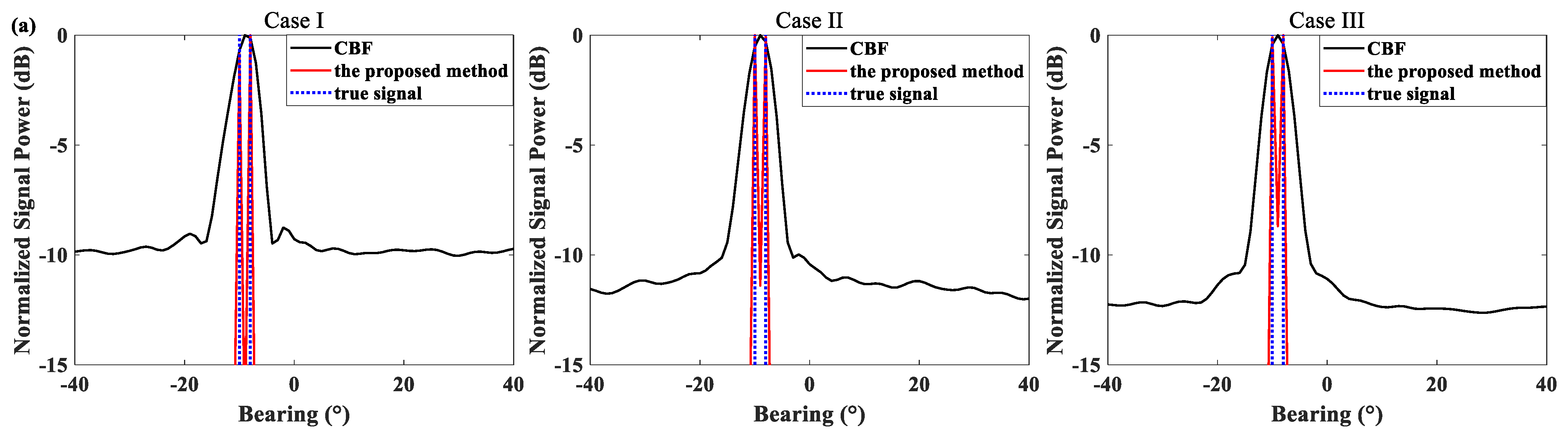
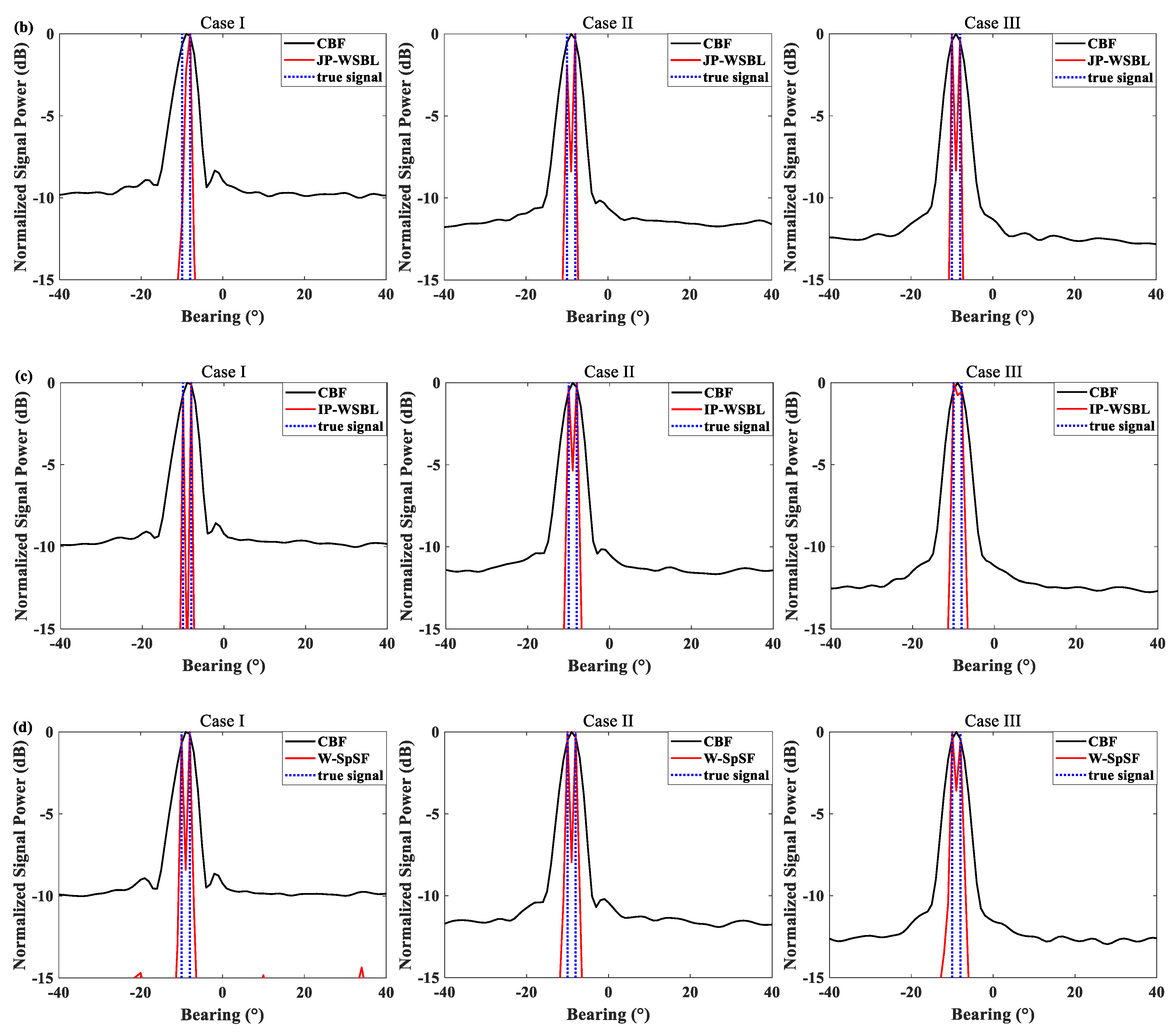
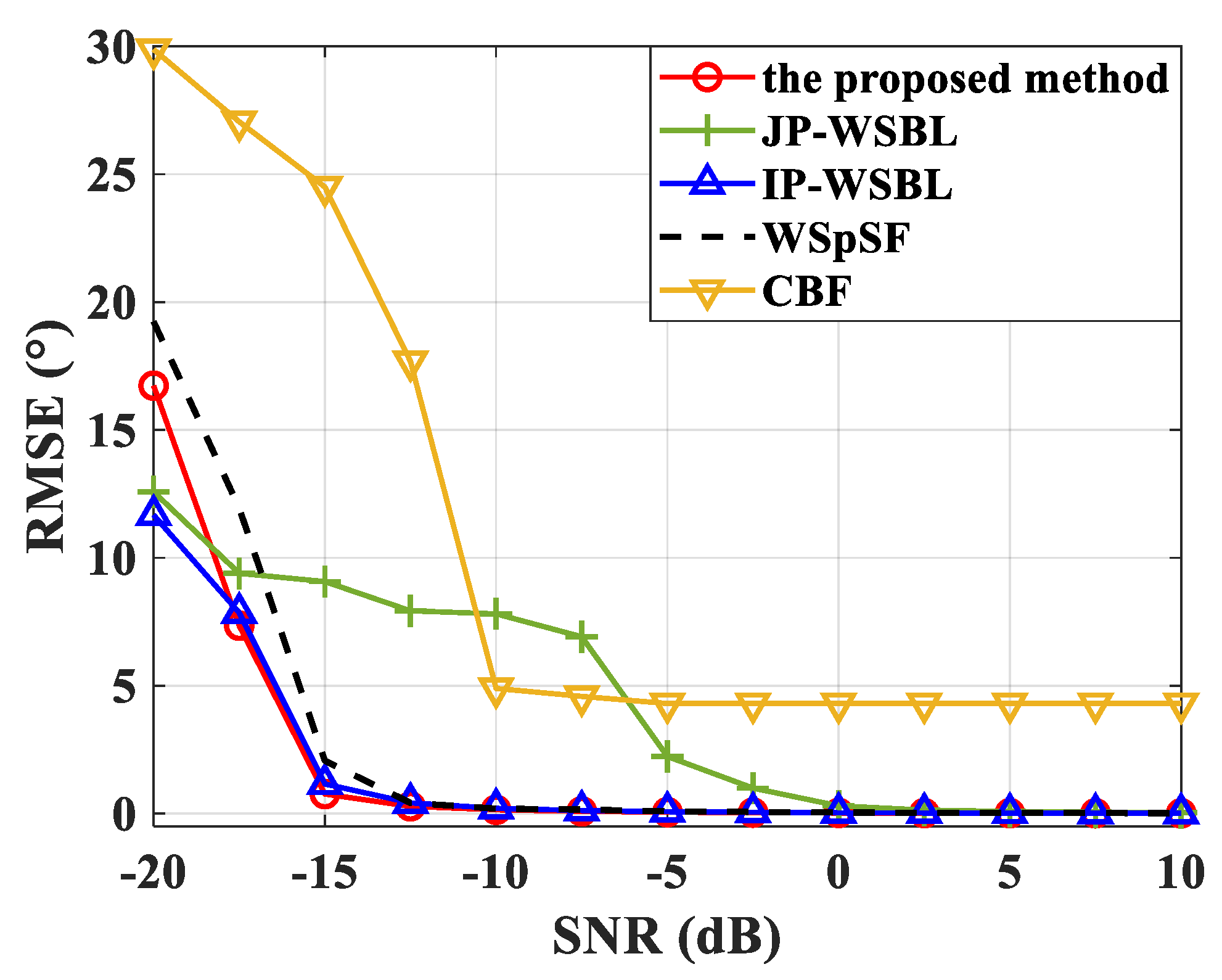
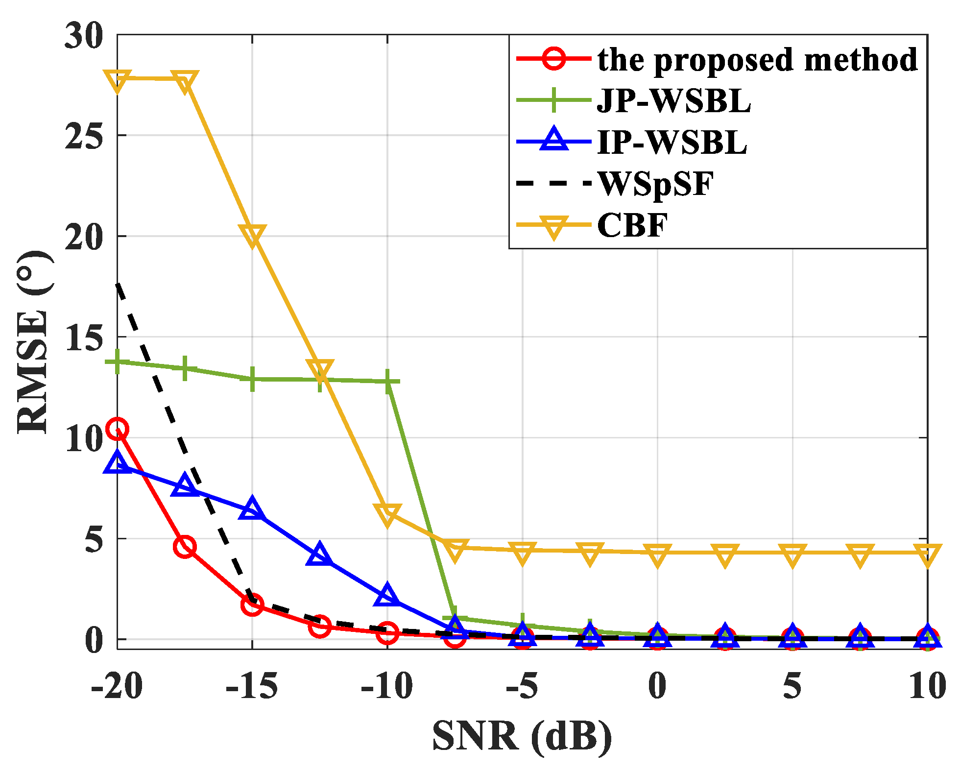
4. Simulation Results

Consider a 32-element uniform linear array (ULA) placed under the sea surface in the simulations. In general, the sound speed in the seawater is considered as 1500 m/s [31]. The array element spacing is 4 m (i.e., the half wavelength of 187.5 Hz). Two far-field sound signals (recorded as Signal1 and Signal2) impinge on the array from −10° and −8° with the assumption of plane wave propagation, where ±90° are defined as the endfire direction. Three different frequency cases are considered as follows:

(1)

Case I: Signal1: [90, 134] Hz, Signal2: [136, 180] Hz. The bandwidth of signals is 44 Hz;

(2)

Case II: Signal1: [90, 160] Hz, Signal2: [110, 180] Hz. The bandwidth of signals is 70 Hz;

(3)

Case III: Signal1: [90, 180] Hz, Signal2: [90, 180] Hz. The bandwidth of signals is 90 Hz.

In the first case, the frequency bands of signals are non-overlapped. In the second case, the signals have partially overlapped bands. In the last case, the signals share the same frequency band. The data are sampled by the acquisition system and the sample frequency is 5 kHz. The received data are divided into 30 segments, i.e., N = 30, with the length of 2500. Then, a 2500-point DFT is applied in each segment, i.e., $\tilde{L}=2500$. The frequency resolution is 2 Hz. The analysis frequency range is from 90 Hz to 180 Hz. The total number of the sub-bands is L = 46.

The performance of the proposed method is compared with the methods in [23,27], and W-SpSF [22]. The method in [27] is a narrowband SBL method. It is used to estimate DOAs in each frequency bin and the results are summed incoherently. Hence, it is recorded as IP-WSBL in the simulation. The method in [23] assigns the same prior in all frequency bins and jointly processes the data in all frequency bins. It is recorded as JP-WSBL. The results of traditional method, i.e., conventional beamforming (CBF) [17], are also shown for comparison purpose. The observed space [−90, 90]° is uniformly discretized into 181 grid points, i.e., Q = 181. The tolerance $\tau$ and $Ite{r}_{\max }$ are set to ${10}^{-3}$ and 3000, respectively. All results are performed in MATLAB on a PC with an Intel Core i7-9700F CPU and an 8 GB RAM.

Figure 3 illustrates the space–frequency map estimation results of the above methods under three different cases by fixing the SNR to −5 dB. The color bar represents the normalized signal power. The row of the bright area gives the DOA information, and the corresponding column provides the signal frequency information in this direction. The results of the proposed method and the W-SpSF are similar to the true values, but the proposed method provides cleaner space–frequency maps. The JP-WSBL achieves a comparable result to the proposed method under the Case III. However, it cannot work well under the first two cases since the sparse supports of the signal vectors in some frequency bins are different and the assumption of a common sparse profile is unsuitable under such conditions. The performance of the IP-WSBL degrades when two signals are in the overlapping frequency bands. Furthermore, the CBF cannot resolve two signals in the overlapping frequency band due to the poor resolution.

Figure 4 illustrates the spectra of the above methods under three different cases. It can be seen that the proposed method and the W-SpSF can estimate two signals under all considered conditions. The IP-WSBL can hardly estimate two signals for Case III since the DOA estimation precision at low frequency bins is poor, affecting the final DOA estimation result. The performance of JP-WSBL degrades under Case I because of the unsuitable assumption on signal sparsity in each frequency bin. Furthermore, the CBF cannot resolve two closely-spaced signals under all considered conditions due to poor resolution.

Then, the performances of above methods on estimation precision are compared from the perspective of the root-mean-square error (RMSE):

$$\mathrm{RMSE}=\sqrt{\frac{1}{KW}{\displaystyle {\sum }_{k=1}^K{\displaystyle {\sum }_{w=1}^W{({\hat{\theta }}_k^w-{\theta }_k)}^2}}},$$

(32)

where ${\hat{\theta }}_k^w$ is the estimated DOA of the kth signal in the wth trial, and W is the total of the Monte Carlo runs. The value of W is set to 200. Figure 5 illustrates the RMSE versus the SNR for Case I. The performances of the proposed method, the IP-WSBL and the W-SpSF are similar to each other and can provide reasonable estimates when SNR ≥ −15 dB. However, the W-SpSF needs to tune a regularization parameter well, which is a difficult task. The JP-WSBL cannot work well at low SNR cases since the assumption in this method is unsuitable under such conditions. The RMSE of the CBF is larger than those of other methods as the SNR increases because it cannot resolve two signals.

Figure 6 shows the RMSE versus the SNR under the condition where the signals have partially overlapped bands. As the overlap of the signal bands increases, two signals are more difficult to be resolved. It is observed that the performances of the proposed method and W-SpSF are nearly unchanged in comparison with the results in Figure 5. The IP-WSBL estimates the DOAs in each frequency bin independently, and the estimation results are not satisfying at the low frequency bins. Hence, it needs higher SNR than the proposed method to provide stable estimates. The RMSE of JP-WSBL is still larger than the proposed method since the sparse supports in different frequency bins are not totally the same. The CBF suffers from low resolution, resulting in large RMSEs in all considered situations.

The RMSE versus the SNR under Case III is shown in Figure 7. Once again, the performances of the proposed method and the W-SpSF are similar to each other. Unlike the W-SpSF, the proposed method gets rid of tuning the hyperparameters manually. Given that the signal vectors share the same sparsity in this simulation, the JP-WSBL assigns the same prior to signal vectors in all frequency bins to make full use of common sparse profile, thus processing the data in all frequency bins jointly. In this manner, the JP-WSBL achieves a comparable performance to the proposed method. The estimation precision of IP-WSBL is affected by large estimation errors in some frequency bins. Hence, it needs higher SNR to achieve high estimation precision, and its RMSE approaches that of the proposed method when the SNR is larger than −5 dB. Furthermore, the RMSE of the CBF is larger than those of other methods due to the low resolution.

Finally, the computational efficiency of each method is compared from the perspective of the mean running time over 200 simulations by fixing SNR to −5 dB.

Table 1. Mean running time of each method under three different frequency cases.

	Case I	Case II	Case III
the proposed method	6.07 s	9.73 s	11.15 s
JP-WSBL	8.30 s	11.76 s	12.36 s
IP-WSBL	7.56 s	10.88 s	12.65 s
W-SpSF	26.49 s	26.28 s	27.14 s
CBF	0.02 s	0.02 s	0.02 s

shows the mean running time of each method under three different frequency cases. The proposed method, JP-WSBL and IP-WSBL iteratively estimate the parameters. The workload in each iteration depends on the updating of ${\Sigma }_{{\stackrel{⌢}{s}}_l}$, which is $O(Q^3)$. However, the proposed method achieves higher computational efficiency than the other two methods mainly because it requires a smaller number of the iterations to converge. The W-SpSF expresses the data in all frequency bins into a matrix, which increases the dimension of the matrix, and the workload is $O(L^3{Q}^3)$ [22]. Hence, it suffers from low computational efficiency. The CBF needs no iteration and avoids matrix inversion. Hence, it achieves the highest computational efficiency, and the workload is $O(Q{M}^2)$. However, it suffers from low resolution.

5. Conclusions

This paper modifies the WSBL to improve its performance under the condition where the signals from different angles have different frequency bands. Given that the signal matrix $[{\stackrel{⌢}{s}}_1(n),\dots ,{\stackrel{⌢}{s}}_L(n)]$ is a row-sparse matrix, and some columns share the different sparse supports when the signals occupy the different frequency bands, different hyperparameters are applied to control the row-sparsity of the signal matrix and the sparsity of the signal vector in each frequency bin. As such, a hierarchical sparse prior is assigned to the signal matrix. The hyperparameters are estimated through VBI to achieve wideband DOA estimation in the Bayesian framework, avoiding the choice of regularization parameter. The proposed method can be regarded as a combination of the JP-WSBL and IP-WSBL. The numerical simulations are performed under the conditions where the signal bands are the same, partially overlapped and non-overlapped. The simulation results verify that the proposed method achieves better performance than the IP-WSBL when the bands of the signals are overlapped, and achieves better performance than the JP-WSBL under the condition that the signals share the different frequency bands.

References

1. Johnson, D.H.; Degraaf, S.R. Improving the resolution of bearing in passive sonar arrays by eigenvalue analysis. IEEE Trans. Acoust. Speech Signal Process. 1982, 30, 638–647. [Google Scholar] [CrossRef] [Green Version]
2. Ren, S.; Ge, F.; Guo, X.; Guo, L. Eigenanalysis-based adaptive interference suppression and its application in acoustic source range estimation. IEEE J. Ocean. Eng. 2015, 40, 903–916. [Google Scholar] [CrossRef]
3. Gerstoft, P.; Xenaki, A.; Mecklenbräuker, C.F. Multiple and single snapshot compressive beamforming. J. Acoust. Soc. Am. 2015, 138, 2003–2014. [Google Scholar] [CrossRef] [PubMed] [Green Version]
4. Zheng, J.; Kaveh, M. Sparse spatial spectral estimation: A covariance fitting algorithm, performance and regularization. IEEE Trans. Signal Process. 2013, 61, 2767–2777. [Google Scholar] [CrossRef]
5. Malioutov, D.; Cetin, M.; Willsky, A.S. A sparse signal reconstruction perspective for source localization with sensor arrays. IEEE Trans. Signal Process. 2005, 53, 3010–3022. [Google Scholar] [CrossRef] [Green Version]
6. Wen, C.; Xie, X.; Shi, G. Off-grid DOA estimation under nonuniform noise via variational sparse Bayesian learning. Signal Process. 2017, 137, 69–79. [Google Scholar] [CrossRef]
7. Zhang, Y.; Yang, Y.; Yang, L.; Guo, X. Root sparse asymptotic minimum variance for off-grid direction-of-arrival estimation. Signal Process. 2019, 163, 225–231. [Google Scholar] [CrossRef]
8. Chen, P.; Chen, Z.; Zhang, X.; Liu, L. SBL-based direction finding method with imperfect array. Electronics 2018, 7, 426. [Google Scholar] [CrossRef] [Green Version]
9. Ling, Y.; Gao, H.; Ru, G.; Chen, H.; Li, B.; Cao, T. Grid reconfiguration method for off-grid DOA estimation. Electronics 2019, 8, 1209. [Google Scholar] [CrossRef] [Green Version]
10. Schmidt, R.O. Multiple emitter location and signal parameter estimation. IEEE Trans. Antennas Propag. 1986, 34, 276–280. [Google Scholar] [CrossRef] [Green Version]
11. Roy, R.; Kailath, T. ESPRIT-estimation of signal parameters via rotational invariance techniques. IEEE Trans. Acoust. Speech Signal Process. 1989, 37, 984–995. [Google Scholar] [CrossRef] [Green Version]
12. Rao, B.D.; Hari, K.V.S. Performance analysis of root-MUSIC. IEEE Trans. Acoust. Speech Signal Process. 1989, 37, 1939–1949. [Google Scholar] [CrossRef]
13. Tipping, M.E. Sparse Bayesian learning and the relevance vector machine. J. Mach. Learn. Res. 2001, 1, 211–244. [Google Scholar]
14. Yang, J.; Liao, G.; Li, J. An efficient off-grid DOA estimation approach for nested array signal processing by using sparse Bayesian learning strategies. Signal Process. 2016, 128, 110–122. [Google Scholar] [CrossRef]
15. Huang, M.; Huang, L. Sparse recovery assisted DOA estimation utilizing sparse Bayesian learning. In Proceedings of the IEEE International Conference on Acoustics, Speech and Signal Processing (ICASSP), Calgary, AB, Canada, 15–20 April 2018. [Google Scholar]
16. Li, S.; Xie, D. Compressed symmetric nested arrays and their application for direction-of-arrival estimation of near-field sources. Sensors 2016, 16, 1939. [Google Scholar] [CrossRef] [Green Version]
17. Kim, H.; Viberg, M. Two decades of array signal parameter estimation. IEEE Signal Process. Mag. 1996, 13, 67–94. [Google Scholar]
18. Wang, H.; Kaveh, M. Coherent signal-subspace processing for the detection and estimation of angles of arrival of multiple wideband sources. IEEE Trans. Acoust. Speech Signal Process. 1985, 33, 823–831. [Google Scholar] [CrossRef] [Green Version]
19. Hung, H.; Kaveh, M. Focussing matrices for coherent signal-subspace processing. IEEE Trans. Acoust. Speech Signal Process. 1988, 36, 1272–1281. [Google Scholar] [CrossRef]
20. Valaee, S.; Kabal, P. Wideband array processing using a two-sided correlation transformation. IEEE Trans. Signal Process. 1995, 43, 160–172. [Google Scholar] [CrossRef] [Green Version]
21. Sellone, F. Robust auto-focusing wideband DOA estimation. Signal Process. 2006, 86, 17–37. [Google Scholar] [CrossRef]
22. He, Z.; Shi, Z.; Huang, L.; So, H.C. Underdetermined DOA estimation for wideband signals using robust sparse covariance fitting. IEEE Signal Process. Lett. 2015, 22, 435–439. [Google Scholar] [CrossRef]
23. Das, A.; Sejnowski, T.J. Narrowband and wideband off-grid direction-of-arrival estimation via sparse Bayesian learning. IEEE J. Ocean. Eng. 2018, 43, 108–118. [Google Scholar] [CrossRef]
24. Das, A. Real-valued sparse Bayesian learning for off-grid direction-of-arrival (DOA) estimation in ocean acoustics. IEEE J. Ocean. Eng. 2021, 46, 172–182. [Google Scholar] [CrossRef]
25. Jiang, Y.; He, M.; Liu, W.; Feng, M. Underdetermined wideband DOA estimation for off-grid targets: A computationally efficient sparse Bayesian learning approach. IET Radar Sonar Navig. 2020, 14, 1583–1591. [Google Scholar] [CrossRef]
26. Hu, N.; Sun, B.; Zhang, Y.; Dai, J.; Wang, J.; Chang, C. Underdetermined DOA estimation method for wideband signals using joint nonnegative sparse Bayesian leaning. IEEE Signal Process. Lett. 2017, 24, 535–539. [Google Scholar] [CrossRef]
27. Tzikas, D.G.; Likas, A.C.; Galatsanos, N.P. The variational approximation for Bayesian inference. IEEE Signal Process. Mag. 2008, 25, 131–146. [Google Scholar] [CrossRef]
28. Themelis, K.E.; Rontogiannis, A.A.; Koutroumbas, K.D. A variational Bayes framework for sparse adaptive estimation. IEEE Trans. Signal Process. 2014, 62, 4723–4736. [Google Scholar] [CrossRef] [Green Version]
29. Yang, J.; Yang, Y.; Lu, J. A variational Bayesian strategy for solving the DOA estimation problem in sparse array. Digit. Signal Process. 2019, 90, 28–35. [Google Scholar] [CrossRef]
30. Yang, L.; Fang, J.; Cheng, H.; Li, H. Sparse Bayesian dictionary learning with a Gaussian hierarchical model. Signal Process. 2017, 130, 93–104. [Google Scholar] [CrossRef] [Green Version]
31. Yang, L.; Hou, X.; Yang, Y. Self-calibration for sparse uniform linear arrays with unknown direction-dependent sensor phase by deploying an individual standard sensor. Electronics 2023, 12, 60. [Google Scholar] [CrossRef]
Figure 1. The signals with (a) the same, (b) non-overlapped and (c) partially overlapped frequency bands. The white and green squares correspond to the absence and presence of a signal, respectively.
Electronics 12 01123 g001
Figure 2. Directed acyclic graph of the hierarchical Bayesian model.
Electronics 12 01123 g002
Figure 3. (a) The true space–frequency map, as well as the estimation results of (b) the proposed method, (c) JP-WSBL, (d) IP-WSBL, (e) W-SpSF and (f) CBF.
Electronics 12 01123 g003aElectronics 12 01123 g003b
Figure 4. The comparison between CBF and (a) the proposed method, (b) JP-WSBL, (c) IP-WSBL and (d) W-SpSF under three different cases.
Electronics 12 01123 g004aElectronics 12 01123 g004b
Figure 5. The RMSE versus the SNR under Case I.
Electronics 12 01123 g005
Figure 6. The RMSE versus the SNR under Case II.
Electronics 12 01123 g006
Figure 7. The RMSE versus the SNR under Case III.
Electronics 12 01123 g007