Binary Neighborhood Coordinate Descriptor for Circuit Board Defect Detection

Abstract

Due to the periodicity of circuit boards, the registration algorithm based on keypoints is less robust in circuit board detection and is prone to misregistration problems. In this paper, the binary neighborhood coordinate descriptor (BNCD) is proposed and applied to circuit board image registration. The BNCD consists of three parts: neighborhood description, coordinate description, and brightness description. The neighborhood description contains the grayscale information of the neighborhood, which is the main part of BNCD. The coordinate description introduces the actual position of the keypoints in the image, which solves the problem of inter-period matching of keypoints. The brightness description introduces the concept of bright and dark points, which improves the distinguishability of BNCD and reduces the calculation amount of matching. Experimental results show that in circuit board image registration, the matching precision rate and recall rate of BNCD is better than that of classic algorithms such as scale-invariant feature transform (SIFT) and speeded up robust features (SURF), and the calculation of descriptors takes less time.

1. Introduction

With the trend of machine vision technology gradually replacing traditional manual visual inspection, optical automatic inspection technology has been widely used in the inspection of industrial products. Deep learning has been applied to the detection of different industrial products and achieved high detection accuracy, such as detection of industrial parts [1], detection of welding defects [2], and detection of manufactured products [3]. The defect detection method based on deep learning can accurately detect the existing defects after training, but it usually needs to be trained again when switching the type of detection object. However, in some small and medium-sized enterprises, inspection equipment is usually used to inspect multiple types of circuit boards, and may be switched frequently. Based on the registration of the reference image and the captured image, the traditional defect detection algorithm can be easily extended to a variety of different types of circuit boards. In such an application scenario, circuit board defect detection algorithms based on traditional image processing are more competitive, so the research in this paper is mainly based on traditional image processing algorithms. The following are some scholars’ research on circuit board defect detection.

Mehmet et al. [4] proposed a defect detection method based on image processing. They used the Y channel information in the YUV color space, extracted features after preprocessing, and detected holes through the Hough transform. Then, the hole number, position, and hole diameter of the holes were matched as features, and the leak holes in each image could be detected. The algorithm targets hole defects and is suitable for circuit boards with holes.

Hua et al. [5] combined good features to track (GFTT) feature detector and SURF descriptor to extract effective features of images and achieved accurate image registration for the first time. Then they used the cross-correlation function to calculate the offset between the reference image and the first registration image for further fine registration. Compared with traditional image registration algorithms, this algorithm had higher robustness and accuracy and could be applied to circuit board defect detection. However, the SURF algorithm takes a long time and is not suitable for direct application in industrial inspection.

Hassanin et al. [6] built a database for all possible components on the circuit board, used the SURF algorithm to register the reference image with the circuit board image, calculated the Exclusive OR (XOR) image, and then performed morphological processing. If a missing item is detected, the SURF feature descriptor of the feature extracted from the difference between the circuit board image and the reference image at the location of the missing component was matched with the features in the database to enable classification of the defect. The algorithm needs to build a database in advance, and the size of the database determines the types of defects that can be detected.

Melnyk et al. [7] proposed a nested set model of the circuit board images: board–chains–contacts–pixels. When detecting defects, a nested set model based on the reference image and circuit board image is first created, and then the relationship between the reference nested set model and the corresponding line points in the circuit board nested set model are compared to detect open circuit and short circuit defects. The algorithm can only detect two kinds of defects, open circuit and short circuit, and cannot detect defects such as mouse bite and pinhole.

Qi et al. [8] proposed a method for detecting welded regions, which extracted the features and centroids of each welded region and completed the detection by comparing it with a reference image. This defect detection algorithm could detect the most common defect types and had the characteristics of low time consumption, high detection accuracy, and high classification accuracy. This algorithm is mainly aimed at the detection of external defects and cannot handle the detection of inner cavity defects.

Guo et al. [9] proposed a circuit board defect detection method based on ORB and image difference. This method used ORB to register the circuit board image with the reference image and performed image preprocessing on the circuit board image to reduce noise and improve image quality. Then, they denoised, morphologically processed, and image binarized the differenced image and finally marked the position of the defect on the circuit board image and counted the total number of defects. However, the algorithm does not work well for circuit boards with complex shapes.

Gao et al. [10] developed an algorithm: performed HAAR wavelet transformation on the XOR image of the reference image and the circuit board image and then removed DC and low-frequency signals and carried out the inverse HAAR wavelet transform and performed XOR operation on the result and the XOR image to obtain the exact position of the defect. The algorithm was able to handle specific frequency ranges and imperfections with lower frequency signals. The algorithm has higher requirements on the input threshold.

The most important step of the circuit board defect detection algorithm is the registration of the reference image and the test image. The classic keypoint based registration algorithm is prone to cross cycle registration when dealing with periodic circuit board images. To solve this problem, we propose a circuit board image registration algorithm, which uses the intercepted template image for template matching to achieve coarse registration and then combines feature matching and random sample consensus (RANSAC) to complete the fine registration of reference images and test images (the captured image of the circuit board, hereinafter referred to as the test image). In particular, we propose the binary neighborhood coordinate descriptor (BNCD) for coarsely registered images, which consists of neighborhood description, coordinate description, and brightness description. BNCD can solve the problem of cross-period matching of keypoints, with fast calculation speed and high precision rate, suitable for industrial production. This descriptor helps us quickly and accurately register test images and realize circuit board defect detection. For the input test image, it can detect defects such as open, short, spurious copper, spur, pinhole, and mouse bite and mark the type and coordinates of the defect.

2. Proposed Algorithm

For the circuit board defect detection algorithm, how to achieve accurate registration of the reference image and the circuit board image is the most difficult and important part. The circuit board contains a large number of periodic structures, and the classic feature-matching algorithm is prone to the problem of cross-period matching, which affects the accuracy of registration. To solve this problem, we propose the BNCD and apply it to the registration of circuit board images. Our proposed image registration method is shown in Figure 1.

The reference image is generated by the Gerber file, and the test image is obtained by the image acquisition system. The position of the circuit board in the two images is different, so a coarse registration is necessary to achieve the initial alignment of the reference image and the test image. Since the inspection equipment performs rotation correction during shooting, the captured test image is not rotated significantly, so in the rough registration part, only the influence of translation needs to be considered (if your test image has obvious rotation, you can perform rotation correction first). The previously intercepted template image and the test image are used to perform template matching based on the gray value and realize the coarse registration. Next, the coarsely registered reference image and test image are segmented to obtain sub-images at corresponding locations. The sub-image is a local image of the circuit board image, which is obtained by dividing the entire circuit board image into small circuit board images. Then, the keypoint-based matching method is used to perform fine registration of the sub-images. In this step, the SURF detector is used to extract keypoints from the reference sub-images and the test sub-images, which can extract a large number of robust keypoints while taking into account the efficiency. Then, BNCD describes the keypoints and quickly finds the matching keypoints through the proposed matching algorithm. Finally, RANSAC is used to eliminate the mismatched pair of keypoints, and the affine transformation matrix is calculated to realize the fine registration. Figure 2 shows the result of registration. The color of the reference image in the Figure 2 is red, the color of the test image is cyan, the overlap part is white, and the misaligned part is red or cyan.

2.1. Coarse Registration Based on Template Matching

The acquired test image has the same orientation and scale as the reference image, so the coarse registration can be performed by template matching. The algorithm flow chart is shown in Figure 3, and the pseudo-code of Algorithm 1 is as follows:

Algorithm 1: Coarse Registration Algorithm Based on Template Matching

Input: test image Itest, reference image Ireference Output: test image after coarse registration Itest’

1: Calculate Itest width w and height h 2: Capture the template image Itemplate from Ireference and record the coordinates C1(x1, y1) of the upper left corner 3: Use Itemplate and Itest for template matching, and record the coordinate with the greatest similarity in the result as C2(x2, y2) 4: Take the pixels from y2-y1 to h rows and x2-x1 to w columns of Itest to get Itest’

Common template matching algorithms include sum of absolute differences (SAD), sum of squared differences (SSD), and normalized cross correlation (NCC) algorithms. In this paper, SSD is used as the method of similarity measurement. The calculation formula of SSD is as follows:

$$R\left(x,y\right)={\displaystyle \sum }_{x^{\prime },y^{\prime }}{\left(T\left(x^{\prime },y^{\prime }\right)-I\left(x+x^{\prime },y+y^{\prime }\right)\right)}^2,$$

(1)

where T (x′, y′) is the pixel value at the template image coordinate (x′, y′); I (x + x′, y + y′) is the pixel value at the input image coordinates (x + x′, y + y′); R (x, y) is the similarity measure at the input image coordinates (x, y). The formula shows that the smaller the result, the greater the similarity and the better the matching degree. In the actual calculation, the position with the smallest result is taken as the matching point.

After the coarse registration based on template matching, the reference image and the test image have achieved preliminary registration, and the various structures of the circuit board have been coarsely aligned. Next, a fine registration is required to achieve higher precision registration.

2.2. Speeded-Up Roubust Feature

SURF, proposed by Herbert Bay [11], is an improved local keypoint detection and description algorithm based on SIFT. Compared with SIFT, SURF accelerates steps such as constructing image pyramids and calculating the main directions of keypoints, which greatly improves the operating efficiency of the algorithm. The steps of the SURF detection keypoint part are as follows:

• Create box filters ($D_{xx}, D_{yy} and D_{xy}$) of different sizes, and then convolve the target image I to obtain the second-order differential responses at each scale.
• Calculate the Hessian determinant image according to (2), and construct an image pyramid.

  $$\det \left(H\right)=D_{xx}{D}_{yy}-{\left(\omega D_{xy}\right)}^2,$$

  (2)

  where $D_{xx}$ is an approximate box filter in x-direction, and $D_{yy}$ and $D_{xy}$ are similar. Formula (2) calculates the approximate value of the determinant of Hessian matrix. $D_{xy}$ multiplied by ω is to balance the error caused by the approximation of box filters. ω is generally taken as 0.9.
• Use non-maximum suppression in the 3 × 3 × 3 neighborhood to preliminarily determine the keypoints, and then perform interpolation operations to determine the precise location and scale of the keypoints.

SURF is fast and can detect high-quality keypoints, so we choose SURF as the keypoint detector to provide the basis for subsequent keypoint descriptor calculations.

2.3. Binary Neighborhood Coordinate Descriptor

Many circuit boards have a large number of similar and periodic keypoints. Classical feature descriptors only contain gradient and pixel value information around keypoints, so it is difficult to distinguish keypoints of different periods. This causes a large number of keypoint pair matching errors and even affects the subsequent image registration. In this paper, BNCD is proposed for the fine registration of coarse-registered binary images. This descriptor can well distinguish similarity and periodic keypoints and improve the precision rate of feature matching. The BNCD consists of three parts: neighborhood, coordinate, and brightness description.

2.3.1. Neighborhood Description

Some scholars combine template matching with keypoint matching to obtain good results. Haifeng Liu et al. [12] use the Harris detector to detect keypoints and then take the neighborhood of keypoints for normalized cross-correlation matching. The pair of keypoints whose calculation result is greater than 0.95 is considered as matching pairs of points. This method of matching keypoints is simple and has a high matching precision rate. However, for each keypoint, it needs to take the neighborhood for similarity measurement, which requires a large amount of calculation and takes a long time. This article takes the neighborhood of keypoints and calculates the similarity measure. Inspired by this article, we propose a method for directly converting neighborhood into descriptors for binary images and then measure the similarity between keypoints by calculating the descriptor distance. Therefore, we propose the neighborhood description of BNCD. As shown in Figure 4, after the key point detection is completed, the neighborhood of the key point is taken, and the binary neighborhood descriptor is calculated. The neighborhood description contains all the value information of the neighborhood of keypoints, so it can be used to distinguish keypoints. The calculation formula of the descriptor $D_N\left(p\right)$ described by the neighborhood is as follows:

$$D_N\left(p\right):={\displaystyle \sum }_{y=0}^{S-1}{\displaystyle \sum }_{x=0}^{S-1}{2}^{Sy+x} \tau \left(N;x, y\right),$$

(3)

where S is the size of the neighborhood. The coordinates of the upper left corner of the neighborhood are (0,0). $\tau \left(N;x, y\right)$ is the calculation rule of the neighborhood N whose size is S × S with the keypoint p as the center, defined as:

$$\tau (N;x,y):=\{\begin{array}{c}1, I\left(x,y\right)>0\\ 0, otherwise\end{array},$$

(4)

where $I\left(x, y\right)$ is the gray value of the point (x,y) in the neighborhood N.

According to (3), the information of the keypoint neighborhood can be converted into a binary descriptor of S × S bits. Simply calculating the Hamming distance can obtain the similarity of two keypoints. The neighborhood description is faster than taking the neighborhood and then measuring the similarity and also has high matching accuracy.

2.3.2. Coordinate Description

Descriptor algorithms usually contain information such as gradients and gray values around keypoints only. If there are similar structures or periodic structures in an image, the descriptors of keypoints at the same position in different periods may be similar or even the same. These similar descriptors cause mismatches of subsequent pairs of keypoints, which has a great impact on the calculation of the transformation matrix. Circuit boards often contain a large number of similar structures and periodic structures, so a large number of mismatches are prone to occur when the existing descriptor algorithms are directly used in the image registration.

In order to reduce the mismatching caused by similar structures and periodic structures, we hope to narrow the matching range of keypoints and no longer match all keypoints in the image, which can reduce the amount of matching calculation and improve the precision rate. One way of thinking is to limit matching by distance. If the distance between two keypoints exceeds the threshold, they are considered not to match; if the distance is less than the threshold, subsequent calculations can be performed. However, if the distance between two points is directly calculated during matching, the amount of calculation is large. To reduce computation, we propose a method to convert coordinate information into binary pattern descriptors and estimate distances between feature points by computing distances between descriptors. In this regard, we propose the coordinate description of BNCD, which adds the coordinate information of keypoints into the descriptor as a feature and can still maintain high precision rate when matching periodic images.

The descriptor of the coordinate description is calculated as follows: record the descriptor of the coordinate description to be added as 2^b bits (where the row and column directions each occupy b bits); divide the image into a $b\times b$ grid, and if the keypoint p is located in the grid of the mth column and the nth row, record the grid coordinates as (m, n). The calculation formula of the descriptor $D_C\left(p\right)$ that defines the coordinate description of point p is:

$$D_C\left(p\right):=2^b{\displaystyle \sum }_{i=0}^{m-1}{2}^i+{\displaystyle \sum }_{j=0}^{n-1}{2}^j$$

(5)

As shown in Figure 5a, the descriptor of the coordinate description is defined as 16 bits, so we divide the image into 8 × 8 grids. Point A is located in column 7, row 3, so the grid coordinates are (7,3). According to (3), the coordinate descriptor is 0111 1111, 0000 0111, a total of 16 bits; the upper 8 bits are the coordinate information in the column direction, and the lower 8 bits are the coordinate information in the row direction. Similarly, it can be calculated that the descriptor of point B in Figure 5b is 0000 0001, 1111 1111, and the descriptor of point C is 1111 1111, 0000 0001. Calculating the Hamming distance, we can determine that the distance between A and B is 11, and the distance between A and C is 3.

With 16-bit descriptor information, the distance between A and B is 11, while the distance between A and C is only 3. Coordinate description can effectively adjust the distance between descriptors according to the actual distance of keypoints on the image. Therefore, keypoints with close distances on the image are easier to match together. Such a mechanism can significantly reduce the impact of similar structures or periodic structures on keypoint matching and improve the precision rate of matching.

It is worth mentioning that directly adding the coordinate description descriptor to the existing binary descriptor can also significantly improve the matching precision rate of keypoint pairs. Figure 6 shows the matching result of a circuit board image; the red line indicates the wrong matching pairs of points, and the green line indicates the correct matching pairs of points. Figure 6a is the result of matching directly using the ORB, and the precision rate of keypoint pairs is 64.0% (correct matches to total matches); Figure 6b is the matching result after adding the coordinate description to the ORB descriptor, and the precision rate of keypoint pairs is 80.4%, which is 15.6% higher than the original algorithm.

2.3.3. Brightness Description

Before performing feature matching, SURF divides the keypoints into two groups according to the positive and negative of the Laplace response, and each group only matches the keypoints of this group. This operation speeds up matching without degrading descriptor performance. Since the value of the response is calculated at the detection stage, this matching method does not require an additional computational cost.

Inspired by the idea of SURF matching, we also want to group the keypoints before matching, and the matching is only performed within the group. Considering that the image we are dealing with is a binary image, we divide the keypoints into two groups directly according to the value of the keypoints. For this, we add brightness descriptions to BNCD and introduce the concept of bright and dark points. Figure 7 shows bright and dark points, which are defined as follows:: if the keypoint is a white pixel, record the keypoint as a bright point, and its brightness descriptor is 1; otherwise record it as a dark point, and its brightness descriptor is 0 (since we are dealing with binary images, there are only white and black pixels in the image). The descriptor calculation formula for brightness description is as follows:

$$B_L\left(p\right):=\{\begin{array}{c}1, I\left(p\right)>0\\ 0, otherwise\end{array},$$

(6)

where $I\left(p\right)$ is the gray value of keypoint p. In this experiment, 2b takes 54, S takes 27, brightness description takes 1 bit, coordinate description takes 54 bits, neighborhood description takes 729 bits, and the total is 98 bytes.

According to the concept of bright and dark points, we can divide the keypoints into two categories. We only match the keypoints of the same category, which can reduce the amount of calculation and improve the speed of matching.

2.3.4. Matching Algorithm for BNCD

Combining the neighborhood description, coordinate description, and brightness description defined above, we obtain BNCD. The calculation descriptor $D_{\mathrm{BNCD}}\left(p\right)$ can describe the keypoints, and the calculation formula for defining the BNCD descriptor is as follows:

$$D_{\mathrm{BNCD}}\left(p\right):=D_L\left(P\right)2^{2b+S^2}+D_C\left(p\right)2^{S^2}+D_N\left(p\right),$$

(7)

where 2b is the number of descriptor bits describe the coordinates; S is the size of the neighborhood.

The matching algorithm of the BNCD is shown in Algorithm 2. When calculating the distance between keypoints, first compare the brightness descriptors $D_b$. If the brightness descriptors are the same, continue the subsequent calculation; otherwise, the pair of points is considered to be mismatched, and the subsequent calculation is not performed. Then calculate the coordinate descriptor $D_c$; if the distance between the coordinate descriptors is less than a given threshold T, continue to calculate the descriptors described by the neighborhood, and complete the calculation of the distance. Otherwise, it is considered that the pair of points does not match, and the distance calculation of the neighborhood description descriptor is not performed.

Algorithm 2: BNCD Matching Algorithm

Input: BNCD of the i keypoint in reference image D(r, i), BNCD of the j keypoint in test image D(t, j), BNCD’s brightness descriptor Db, BNCD’s coordinate descriptor Dc, threshold for the distance of the coordinate descriptor T, calculate the distance between two descriptors Dist() Output: Matching result M, M(i) = j means that i keypoint of the reference image matches j keypoint of the test image

1: Count the number of keypoints in reference image m, count the number of keypoints in test image n 2: for i = 1, 2, …, m do 3:       distmin ← 1000 4:       for j = 1, 2, …, n do 5:             if Dist(Db(r, i), Db(t, j)) == 0 then 6:                   if Dist(Dc(r, i), Dc(t, j)) < T then 7:                          if Dist(D(r, i), D(t, j)) < distmin then 8:                                distmin ← Dist(D(r, i), D(t, j)) 9:                                M(i) = j

The brightness descriptor can divide the keypoints into two types: bright points and dark points. Calculating the descriptor of the brightness description first can ensure that each type of keypoint is only matched with the same type of keypoint, preventing different types of points from being matched and reducing the matching calculations.

Then, calculate the distance between the coordinate descriptors, and decide whether to continue to calculate the neighborhood descriptor according to whether the distance is less than a given threshold. This judgment can ensure that the actual distance of the matched keypoints on the image is less than the threshold and can avoid the occurrence of matching errors due to the periodic structure. As shown in Figure 8, when the threshold of the coordinate descriptor T = 1, A is matched with a keypoint in a grid, and A can only be matched with A’. When T = 3, A is matched with feature points within 12 grids, and A can be matched with A’ and B’. As T increases, the actual range of matching also increases, and more keypoints can be matched. By setting an appropriate T, the matching range can be limited to prevent the keypoints of this period from being matched to other periods. Constrained by coordinate descriptors, BNCD outperforms state-of-the-art descriptors for matching on periodic images.

The pairs of keypoints that meet the requirements of brightness descriptor and coordinate descriptor continue to calculate the distance of the neighborhood descriptor and finally determine the matching point pair according to the shortest distance.

The BNCD matching algorithm can prevent the wrong matching between dark points and bright points and prevent two points with a large actual distance difference on the image from being matched. The distance of the entire descriptor is only calculated if the pairs of keypoints are both dark or bright and the actual distance on the image is small. This matching algorithm can reduce the amount of calculation and improve the precision rate of matching.

2.3.5. BNCD Failure Situation

The design purpose of the coordinate descriptor in BNCD is to limit the matching range of keypoints. In the case of coarse registration of images, the limitation of coordinate description can prevent matching of keypoints of different periods, reduce the amount of calculation, and improve the precision rate of matching. However, in the absence of coarse registration, the matched target keypoints may be outside the restricted range, and the constraints of the coordinate descriptor become a negative impact, resulting in failure to match with the correct keypoints.

Figure 9 shows the matching results of SURF descriptors and BNCD without coarse registration, and the SURF feature point detector is used uniformly. The test image is rotated 180 degrees in Figure 9a,b, and the test image is rotated 90 degrees clockwise in Figure 9c,d. The results show that the precision rate of matching using BNCD is low without rough registration, and a large number of mismatches occur.

To sum up, before using BNCD, the image should be roughly registered. This step has been completed in 2.1 in this article, so there is no need to worry about the BNCD failure of the circuit board image during the registration process.

2.4. RANSAC

After calculating the matching pairs of points, we need to estimate the transformation model from the test image to the reference image. According to the transformation between the actual test image and the reference image, we use affine transformation as the transformation model. For this, we calculate the transformation matrix from the test image to the reference image according to the RANSAC algorithm [13]. The pseudo code Algorithm 3 of RANSAC is as follows:

Algorithm 3: Random Sample Consensus Algorithm

Input: number of iterations kmax, confidence interval η0, matching result M Output: optimal transformation matrix Hbest

1: Count the number of matches N in M 2: k ← 0, Imax ← 0 3: while k < kmax do 4:       Randomly sample minimal subset of 3 pairs of point from M 5:       Estimate affine transformation matrix Hk 6:       Calculate the set of inner points Ik 7:       if |Ik| > Imax then 8:             Hbest ← Hk 9:             Imax ← |Ik| 10:            kmax ← log(1 − η0)/log(1 − ε3), using ε ← |Ik|/N 11:       k = k + 1

The RANSAC algorithm can be used to eliminate mismatches, obtain an affine transformation matrix, and realize fine registration between the test sub-image and the reference sub-image. So far, the above algorithm has realized the registration work of the test image and laid the foundation for the subsequent defect detection algorithm.

3. Results and Discussion

The configuration of the computer used in this experiment is as follows: Win10, AMD Ryzen 7 4800H with Radeon graphics processor, main frequency 2.90 GHz, 16G memory. The code was programmed in Visual Studio 2019 using the OpenCV library, version 4.5.5.

3.1. Comparison with State-of-the-Art Descriptors

In this section, we used test image collected by the image acquisition system and reference image generated by Gerber file to verify the matching precision rate, recall rate, and speed of BNCD. For evaluation purposes, we rely on three straightforward metrics, elapsed CPU time, recall rate and recognition rate. The former is simply averaged measured wall clock time over many repeated runs. The definitions of the latter two refer to paper [14]. The number of correct and incorrect matches is determined by the projection error PE, which is defined as the Euclidean distance calculated between the matched keypoint and the ground truth keypoint (correct match). In our experiments, we experimentally fixed the projection error to PE = 3 [15]. We counted the computation results of well-known feature descriptors (namely SURF, SIFT, ORB, BRISK, KAZE, AKAZE, FREAK, and BEBLID) on our circuit board images. Each original descriptor is built on top of its keypoint detector (FREAK is built on top of AGAST detector, and BEBLID is built on top of ORB detector), and we decided to output the results for each of these detectors for a fair comparison. For example, when BNCD was applied to the keypoints detected by SURF, we call it SURF + BNCD.

$$1-Percision=\frac{\#false matches}{\#correct matches+\#false matches}$$

(8)

$$Recall=\frac{\#correct matches}{\#correspondences}$$

(9)

We used the nearest neighbor algorithm to match the classic descriptors, used the BNCD matching algorithm proposed above to match the BNCD, and take the 500 keypoints with the largest response for each image. Since each keypoint matching only one keypoint, the recall rate does not approach 1, and the precision rate does not approach 0.

As shown in Figure 10, after the description proposed in this paper was combined with the keypoint extraction algorithm of the classic algorithm, its precision rate and recall rate are significantly improved, both of which were higher than the original algorithm. The main reason for the low precision rate of the classic algorithm in the circuit board images is that there are a large number of periodic structures in the circuit board image, and there are a large number of cross-period matches during matching, resulting in a low precision rate. The BNCD proposed in this paper takes into account the characteristics of more periodic structures in circuit board images, and adds coordinate descriptions, so it can maintain a high precision rate and recall rate.

Figure 11 shows the time-consuming calculation of 500 descriptors. Descriptor algorithms based on histogram of oriented gradient (HOG) such as SIFT, SURF, KAZE, and AKAZE take a long time, and the KAZE algorithm takes the longest time, exceeding 1200ms. Local binary pattern (LBP) descriptor algorithms such as ORB, BRISK, FREAK, and BEBLID take less time, and the time-consuming of BEBLID algorithm is the shortest, which is 5.03 ms. The BNCD proposed in this paper takes the shortest time, 1.72 ms, which is significantly shorter than the HOG descriptor, and has obvious advantages over the LBP descriptor. This is related to the calculation method of the BNCD. The calculation of the BNCD is simple and fast, and time-consuming operations such as rotation and image gradient calculation are omitted.

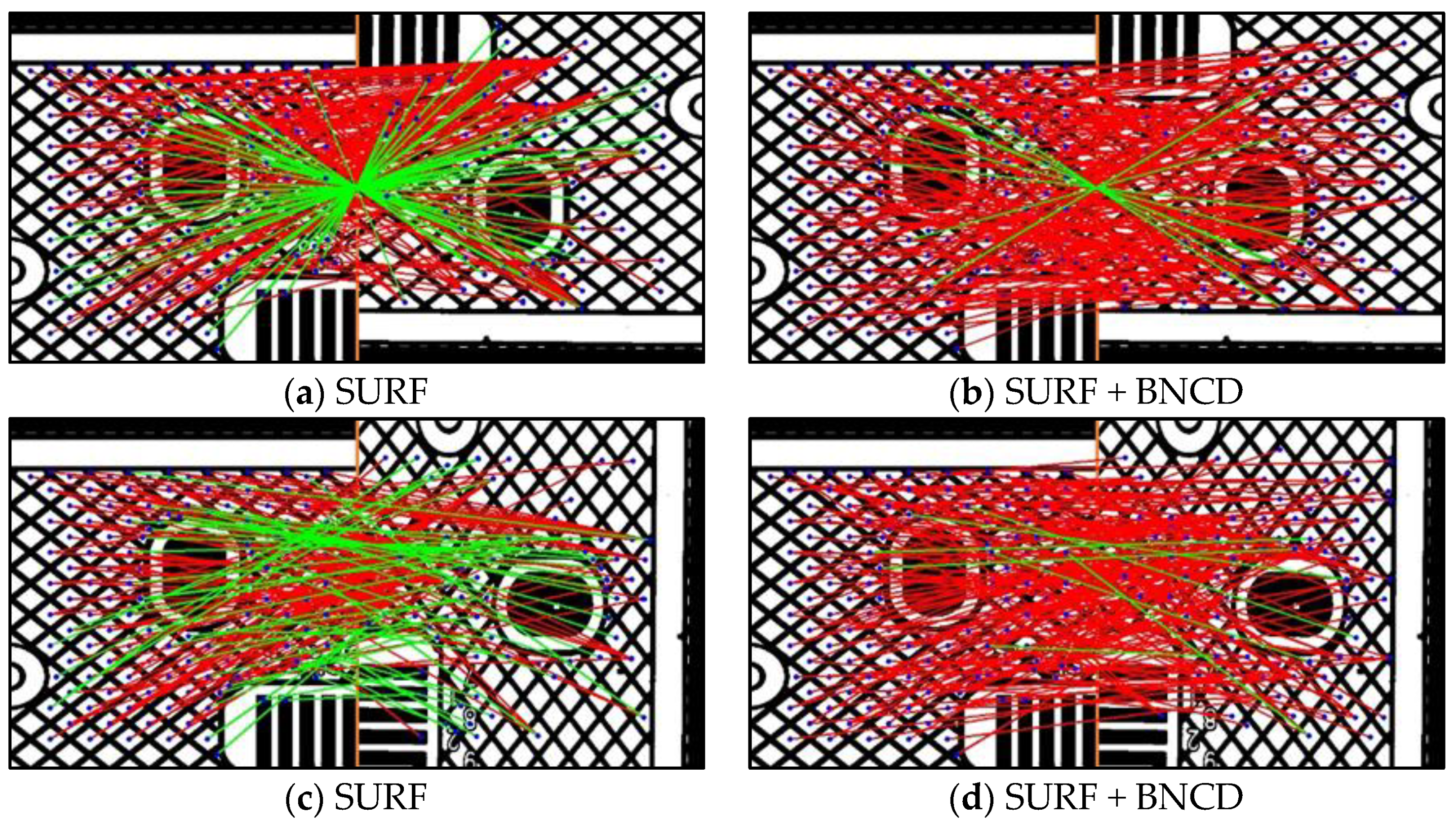
In Figure 12, we show the matching results of some classical descriptors and BNCD. Green and red lines respectively indicate correct and incorrect matches. There are a large number of periodically repeated diamond-shaped structures in this test image. It is difficult to distinguish them with classic descriptors, and a large number of mismatches appear. Due to the limitation of coordinate description, BNCD can guarantee high matching precision rates.

3.2. The Influence of Coordinate Description and Brightness Description on BNCD

Figure 13a shows the effect of different descriptions on the precision–recall curve. We extract keypoints using a SURF detector and only use the top 500 keypoints with the largest response. Experimental results show that brightness descriptions have little impact on the matching effect, and the descriptors without brightness descriptions can still maintain a high precision rate. However, the brightness description can divide the keypoints into two categories, reduce the amount of calculation, and improve the matching speed. Therefore, brightness description is also necessary for the BNCD. The coordinate description has a great influence on the matching effect. After removing the coordinate description, the best matching precision rate is less than 20%, and the best recall rate is less than 30%. In general, coordinate description can improve the distinguishability of keypoints, thereby improving the precision rate of matching. The brightness description can reduce the calculation amount of matching, thereby improving the speed of matching.

3.3. Circuit Board Inspection Results

After the sub-image registration is completed, the reference image and the test image are differentiated to detect possible defects. Morphological operation is performed on the difference results to remove the influence of minor errors and merge the same defect, so as to determine the coordinates of defects on the sub-image. According to the position of the sub-image in the whole circuit board image, the defect coordinates on the sub-image are converted to the coordinates on the whole circuit board image. Finally, defect classification is carried out to complete defect detection. The types of circuit board defects detected are shown in Figure 14.

For circuit board detection, we considered the influence of time and matching effect, chose SURF as the detector and BNCD as the descriptor, and combined them into the feature detection part of fine registration. The test set uses 50 physical images of the circuit board taken in the factory, the test image size is 7864 × 12,800, and the circuit board size is 255 mm × 512 mm. The number of defects in actual production is small. In order to verify the effectiveness of the algorithm, some defects such as short, open, and spurious copper are artificially constructed. The reference image is generated from a Gerber file, and the size of the reference image is 6946 × 12,766. Detection results are measured by true positive (TP), false positive (FP), false negative (FN), true positive rate (TP rate), and false positive rate (FP rate), where TP means that the test result is a defect, but it is actually a defect; FP means that the test result is a defect, but it is not actually a defect; FN means that the test result is not a defect, but it is actually a defect. The calculation formulas of FN, TP rate, and FP rate are as follows:

$$FN=Total defects-TP$$

(10)

$$TP rate=\frac{TP}{Total defects}$$

(11)

$$FP rate=\frac{FP}{FP+TP}$$

(12)

The data in

Table 1. Circuit board detect results.

Defect Type	Total Defects	TP	TP Rate (%)	FP	FP Rate (%)	FN
Short	91	88	96.7	6	6.38	3
Spurious copper	78	78	100	0	0	0
Spur	81	80	98.77	2	2.44	1
Open	71	69	97.18	0	0	2
Pinhole	66	66	100	0	0	0
Mouse bite	112	112	100	2	1.75	0

show that the average TP rate is 98.8% and the average FP rate is 1.99%, which can meet the needs of industrial production, indicating that the BNCD proposed in this article can be applied to circuit board defect detection.

4. Conclusions

In this paper, we propose a new descriptor, BNCD, for the fine registration of circuit board binary images, which includes neighborhood, coordinate, and brightness descriptions. The neighborhood description is calculated from the pixel values around the keypoint, the coordinate description is calculated from the actual position of the keypoint in the image, and the brightness description is calculated from the gray level of the keypoint. In addition, we propose a corresponding matching algorithm, which is calculated step by step according to different descriptions, and the subsequent distance calculation is not performed for unmatched pairs of keypoints so as to improve the precision rate of matching. The experimental results show that the matching precision rate and time consumption of BNCD in coarse registration of binary images are significantly better than other descriptors, and it is not affected by periodic structures. BNCD is suitable for industrial defect detection of circuit board, with robustness and real-time performance.