Clustered Federated Learning Based on Momentum Gradient Descent for Heterogeneous Data

Abstract

Data heterogeneity may significantly deteriorate the performance of federated learning since the client’s data distribution is divergent. To mitigate this issue, an effective method is to partition these clients into suitable clusters. However, existing clustered federated learning is only based on the gradient descent method, which leads to poor convergence performance. To accelerate the convergence rate, this paper proposes clustered federated learning based on momentum gradient descent (CFL-MGD) by integrating momentum and cluster techniques. In CFL-MGD, scattered clients are partitioned into the same cluster when they have the same learning tasks. Meanwhile, each client in the same cluster utilizes their own private data to update local model parameters through the momentum gradient descent. Moreover, we present gradient averaging and model averaging for global aggregation, respectively. To understand the proposed algorithm, we also prove that CFL-MGD converges at an exponential rate for smooth and strongly convex loss functions. Finally, we validate the effectiveness of CFL-MGD on CIFAR-10 and MNIST datasets.

1. Introduction

Recently, machine learning [1,2] has been successfully applied in distinct fields, such as computer vision [3], voice recognition [4], and natural language processing [5]. Large amounts of data are required in these data-intensive applications. Nonetheless, data are generally generated and stored on personal terminal devices, such as mobile phones, personal computers, wearable devices, etc. Traditional machine learning collects data in a centralized manner and stores the data in a data center. However, this approach no longer meets the requirements for privacy. Protecting privacy [6] while collecting large amounts of data remains a key issue. For this reason, federated learning (FL) [7,8,9] was proposed by Google in 2016. FL, as a promising edge-learning framework [10], has received widespread attention as a distributed paradigm. FL enables multiple clients to collaboratively train a global model without sharing or exchanging their own private data. During the process of model training, information related to the model or information in encrypted form can be exchanged between parties. This exchange does not expose any protected private parts of the data on each client, and efficient learning can be carried out between multiple participants and compute nodes. The emergence of federated learning can effectively balance the contradiction between benefit and privacy, solving the problem of data aggregation [11]. However, because of the highly decentralized system architecture of FL, it also encounters a crucial challenge—data heterogeneity [12,13].

In FL, data heterogeneity mainly stems from the fact that each client participating in the training is independently distributed, but does not follow the same sampling method, resulting in non-independent identically distributed (non-i.i.d.) data  [14,15]. This problem leads to a steep decline in model accuracy, and how to mitigate the adverse effects of non-i.i.d. is an open question. References [16,17] proposed the k-means clustered algorithm based on FL. However, the k-means clustering algorithm can only be used on convex datasets, meaning that the shape of the k-means cluster can only be spherical, which cannot be generalized to arbitrary shapes. Additionally, it heavily depends on the value of k, and when the data amounts are large, we cannot judge in advance. Reference [16] used the cosine distance to measure the similarities between network data objects. Reference [18] proposed StoCFL, a novel clustered federated learning approach for addressing generic non-IID issues. They also employed cosine distance to measure the similarity of clients. However, their method did not account for differences in data values, in practice. Reference [17] proposed one-shot federated clustering by using k-means to cluster the clients [19]. Nevertheless, with the k-means method, is difficult to determine the value of k in practical applications. In addition, some recent works have utilized user-clustered methods to exploit data heterogeneity.

Reference [20] proposed a user-clustered algorithm based on the similarity between clients, Reference [21] investigated a user-clustered algorithm based on model parameter distance, and Reference [22] developed a user-clustered algorithm based on the weighted sum of clients. The aforementioned works based on the user-clustered algorithm merely considered the conditions to achieve clustering; however, the convergence rate has rarely been a concern. Additionally, Reference [23] proposed the IFCA algorithm to divide clusters by minimizing loss functions and provided convergence analysis, but the convergence rate is not desirable. Reference [24] introduced a new clustered FL algorithm based on weighted clients and discussed the convergence analysis. However, in cases with multiple missing attributes, different weights must be assigned to the missing combinations of different attributes, which significantly increases the calculation difficulty and reduces the prediction accuracy. Despite the numerous works that have utilized clustered methods to address data heterogeneity in FL, the convergence rate of clustered algorithms in FL remains an urgent problem.

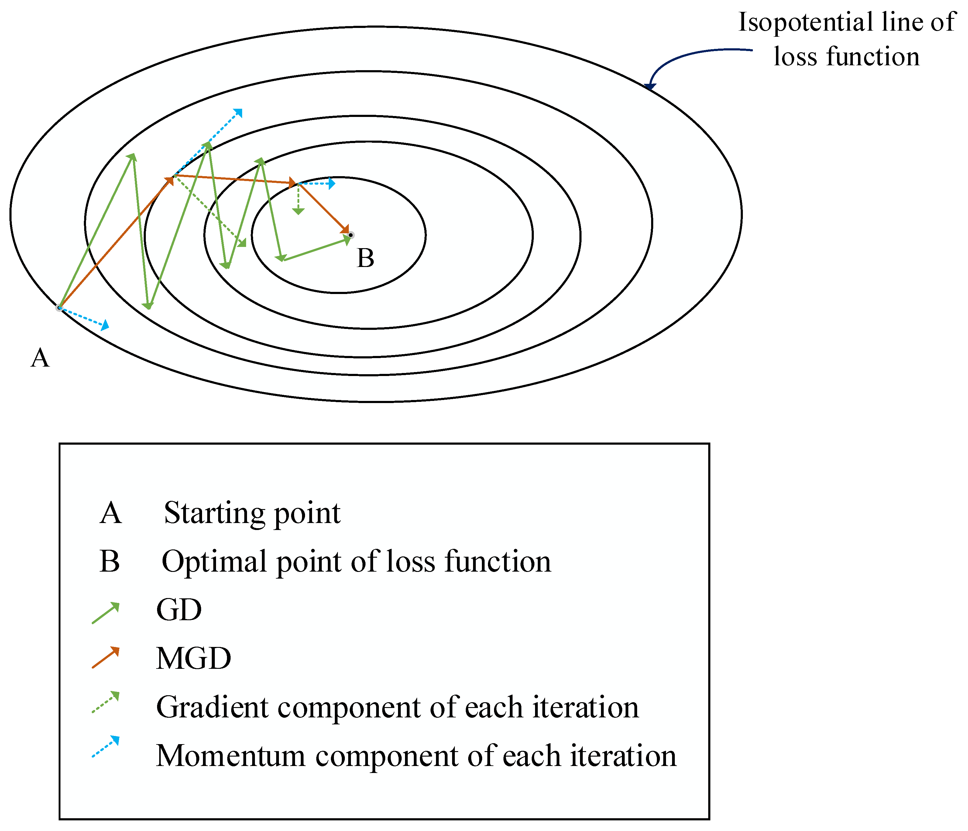
Currently, as an acceleration technique, the momentum method is widely used to improve the convergence rate of the optimization algorithm [25,26,27]. Common algorithms include momentum gradient descent (MGD) [28] and adaptive algorithms, such as AdaGrad [29], Adam [30,31,32], as well as some subsequently improved algorithms  [33,34]. By incorporating momentum, the previous gradient is reused, and a cumulative discount is applied to it. By modifying the direction of gradient improvement, the influence of the previous gradient on the current gradient is used to accelerate the training speed of the model. The momentum method used in model training can effectively reduce the training time and accelerate the convergence of the algorithm. For instance, Polyak’s momentum GD is a classic momentum GD used to train neural networks, which has good generalization and fast convergence [35,36,37]. As shown in Figure 1 [25], the MGD algorithm can accelerate gradient descent and alleviate oscillation amplitude. In recent years, the momentum method has been widely used in optimization algorithms to compensate for the slow convergence in FL. Nevertheless, research on the application of momentum methods in federated learning based on clustered algorithms is lacking.

In order to accelerate the convergence of the algorithm and alleviate data heterogeneity, we propose a framework named clustered federated learning based on momentum gradient descent (CFL-MGD), as shown in Figure 2. It combines Polyak’s momentum [38] and clustered methods for use in federated learning. The learning process involves selecting locally optimal parameters by minimizing the local loss function and dividing clients with the same learning parameters into a cluster. The momentum gradient descent algorithm is then used to update the model during the training process.

The essential contributions of this paper are as follows:

• We propose clustered federated learning based on momentum gradient descent to address the data owned by clients in federated learning, where the data are habitually non-independently identically distributed.
• We establish a convergence guarantee for the proposed CFL-MGD algorithm in a convex setting and show that our algorithm can achieve exponential convergence.
• We experimentally show that the proposed algorithm can perform well in non-convex settings, such as neural networks.

The abbreviation interpretation is shown in

Table 1. Abbreviation summary table.

Abbreviation	Definition
m	the number of clients
P	total number of clusters
$C_p$	the p-th of the cluster
$M_t$	randomly select participating clients
Y	a subset of the data points on the i-th client
$\left|Y\right|$	the number of data points on the i-th client
$D_i,\left|D_i\right|$	the dataset and dataset size of client i
${\varphi }_i(\chi ;Y)$	the i-th client’s loss function
${\varphi }_p\left(\chi \right)$	the p-th cluster loss function
$\left[P\right]$	the set of integers $\{1,2,\dots ,P\}$
$\parallel ·\parallel$	the ${\ell }_2$ norm of vectors
$r_{i,p}$	$r_{i,p}=1$ if $i\in C_p$ else $r_{i,p}=0$
$g_i$	unbiased gradient estimation of $\nabla {\varphi }_i\left(w\right)$
$\eta ,\beta$	learning rate
T	the number of epochs

.

The remainder of this paper is established as follows. In Section 2, we introduce the related work and define the preliminaries in Section 3. Then, we propose the algorithm in Section 4 and analyze theoretical guarantees in Section 5. Next, in Section 6, we carefully verify our theoretical analysis through experiments. Ultimately, we conclude this paper in Section 7.

2. Related Work

Federated learning faces the challenge of data heterogeneity due to its highly decentralized architecture. Numerous studies have been conducted to mitigate this issue. Clustered FL was proposed in [20] as a solution for processing data heterogeneity. Subsequently, many studies have shown that clustered federated learning is an effective way to address the problem of data heterogeneity [14,39,40]. It divides clients into two partitions based on the cosine similarity between clients. Reference [23] proposed the IFCA algorithm to estimate cluster classes by minimizing the loss functions. In our paper, our algorithm is similar to IFCA, but we delivered a major contribution to the convergence rate of the algorithm. Meanwhile, the convergence of our algorithm and generalization of test data are guaranteed.

2.1. FL and Data Heterogeneity

Federated learning consists of a central server and multiple clients. In FL, users’ personal devices are often in various regions and industries, so the data owned by each client are non-i.i.d., resulting in data heterogeneity. In order to alleviate the problem, Reference [41] proposed a combinatorial approach involving personalized federated learning. However, when extended to extensive networks, this approach is limited to convex targets. User clustering methods are proposed in [42], but the parallel algorithm of user clustering based on assumption loss is not common, and convergence analysis has not been discussed. Reference [21] proposed a user-clustered algorithm based on the model parameter distance, FeSEM, but the convergence rate of the algorithm was not analyzed. Reference [17] proposed one-shot federated clustering by using the clustering method (using local k-means), but it only performed one round of communication, resulting in poor accuracy. Clustered federated learning (CFL) was proposed in [20]; it divided clients into two partitions based on the similarity between clients, but it paid little attention to the convergence rate. Reference [43] proposed proportional fairness-clustered federated learning and provided a detailed convergence analysis, but the convergence effect was closely related to the assumption that global variance is bounded.

2.2. Momentum Method

As an acceleration technique, the momentum method is widely used to improve the convergence rate of optimization algorithms. It is a special first-order optimization method based on the classical gradient descent [25] method by adding momentum. Momentum algorithms are divided into two classes: the heavy-ball momentum method proposed by Polyak in 1964 [38], and the Nesterov-accelerated gradient (NAG) proposed by Nesterov in 1983 [44]. Ghadimi et al. conducted in-depth studies on the convergence of the heavy-ball method and gave the average and individual convergence rates under the condition of a smooth objective function [45]; however, they did not reach the optimal convergence rate. Reference [46] established an algorithm framework with multiple parameters, which uniformly processed the gradient descent method, the heavy-ball method, and the NAG method. In this framework, different optimization algorithms could be obtained by setting different parameters. The momentum method has been widely used to improve the convergence rate of optimization algorithms. Therefore, it is feasible to apply momentum in federated learning based on clustered algorithms.

3. Preliminaries

Let us consider a clustered federated learning framework with P clusters and m clients. We have

$$\underset{{\chi }_p}{min}{\varphi }_p\left({\chi }_p\right)=\frac{\left|D_p\right|}{\left|D\right|}\sum _{i\in C_p^{*}}{\varphi }_i\left({\chi }_p\right),$$

(1)

where $p\in \left[P\right]$. Our goal is to find solutions ${\left\{{\chi }_p\right\}}_{p=1}^P$ that approach ${\chi }_p^{*}=arg\underset{\chi }{min}{\varphi }_p\left(\chi \right)$. In this paper, we assume that m clients have P different data distributions, $D_1,D_2,\dots ,D_P$, and are divided into P disjoint clusters, $C_1^{*},C_2^{*},\dots ,C_P^{*}$, and every client $i\in C_p^{*}$ owns n i.i.d. data point $y^{i,1},\dots ,y^{i,n}$. In particular, we define the i-th client’s loss function

$${\varphi }_i({\chi }_p;Y)=\frac{1}{\left|Y\right|}\sum _{y\in Y}f({\chi }_p;y),$$

(2)

where $Y\subseteq \{y^{i,1},\dots ,y^{i,n}\}$ represents the set of data points by the i-th client. This loss function is defined as $f({\chi }_p;y):\chi \to {\mathbb{R}}^d$ with respect to the data point y. ${\varphi }_i\left({\chi }_p\right)$ is the local lost function. The CFL-MGD learning process is as follows: We adopted two optimization schemes, i.e., average gradient and aggregate model parameters. Foremost, we set initial values for ${\mathbf{u}}_i^{\left(0\right)}$, ${\chi }_i^{\left(0\right)}$ and ${\chi }_p^{\left(0\right)},p\in \left[P\right]$.

Local Updating:

(a)

For gradient averaging, we first compute the (stochastic) gradient $\nabla {\varphi }_i\left({\chi }_p^{\left(t\right)}\right)$ and update the momentum

$${\mathbf{u}}_i^{\left(t\right)}=\beta {\mathbf{u}}_i^{(t-1)}+\nabla {\varphi }_i\left({\chi }_p^{(t-1)}\right).$$

(3)

(b)

For model averaging, local updates are performed in parallel on each client:

$$\begin{array}{c}\hfill {\mathbf{u}}_i^{\left(t\right)}=\beta {\mathbf{u}}_i^{(t-1)}+\nabla {\varphi }_i\left({\chi }_i^{(t-1)}\right)\\ \hfill {\chi }_i^{\left(t\right)}={\chi }_i^{(t-1)}-\eta {\mathbf{u}}_i^{\left(t\right)}.\end{array}$$

(4)

According to (4), node i optimizes its loss function ${\varphi }_i\left(\chi \right)$ by performing MGD. The reason for using MGD is to improve the convergence of the algorithm.

Global aggregation: client i transmits ${\mathbf{u}}_i^{\left(t\right)}$, ${\chi }_i^{\left(t\right)}$ and $\nabla {\varphi }_i\left({\chi }_p^{\left(t\right)}\right)$ to the central server, which averages the received parameters from m clients to obtain the cluster parameters, ${\mathbf{u}}_p^{\left(t\right)}$ and ${\chi }_p^{\left(t\right)}$, respectively. There are two approaches to this aggregation rule:

(a)

Gradient averaging:

$$\left\{\begin{array}{c}{\chi }_p^{\left(t\right)}={\chi }_p^{(t-1)}-\frac{\eta }{m}{\displaystyle \sum _{i\in M_t}}{r}_{i,p}{\mathbf{u}}_i^{\left(t\right)}\hfill \\ {\mathbf{u}}_p^{\left(t\right)}=\frac{{\displaystyle \sum _{i\in M_t}}{r}_{i,p}{\mathbf{u}}_i^{\left(t\right)}}{{\displaystyle \sum _{i\in M_t}}{r}_{i,p}}.\hfill \end{array}\right.$$

(5)

(b)

Model averaging:

$$\left\{\begin{array}{c}{\chi }_p^{\left(t\right)}={\displaystyle \sum _{i\in M_t}}{r}_{i,p}{\chi }_i^{\left(t\right)}/{\displaystyle \sum _{i\in M_t}}{r}_{i,p}\hfill \\ {\mathbf{u}}_p^{\left(t\right)}=\frac{{\displaystyle \sum _{i\in M_t}}{r}_{i,p}{\mathbf{u}}_i^{\left(t\right)}}{{\displaystyle \sum _{i\in M_t}}{r}_{i,p}}.\hfill \end{array}\right.$$

(6)

Here, $r_{i,p}$ is the one-hot encoding vector. The central server sends the aggregated cluster parameters ${\mathbf{u}}_p^{\left(t\right)}$ to i with $r_{i,p}=1$, and broadcasts the parameters ${\chi }_p^{\left(t\right)}$ for the next iteration. If we let ${\chi }_i^{(-1)}={\chi }_i^{\left(0\right)}$, then (4) can be equivalently written as the following single variable version

$${\chi }_i^{\left(t\right)}={\chi }_i^{(t-1)}-\eta \nabla {\varphi }_i\left({\chi }_i^{(t-1)}\right)+\beta ({\chi }_i^{(t-1)}-{\chi }_i^{(t-2)}),$$

(7)

where the term $\beta ({\chi }_i^{(t-1)}-{\chi }_i^{(t-2)})$ is habitually referred to as Polyak’s momentum.

4. CFL-MGD Algorithm

A detailed introduction of the algorithm is given in this section, namely clustered federated learning based on momentum gradient descent (CFL-MGD). The primary idea is to cross-iterate the minimization loss function and evaluate the category of clusters. There are two processes: initially, the server broadcasts P parameters and randomly selects participating clients. Next, each client calculates and selects the model parameters that minimize the local loss function

$$\widehat{p}=arg\underset{p\in \left[P\right]}{min}{\varphi }_i\left({\chi }_p^{\left(t\right)}\right).$$

(8)

For gradient averaging, each client calculates the gradient $\widehat{\nabla }{\varphi }_i\left({\chi }_{\widehat{p}}^{\left(t\right)}\right)$ and updates the momentum buffer. For model averaging, each client performs MGD using (4). Ultimately, the solution of each cluster is updated in parallel and the next iteration continues until the end of the loop, using (5) or (6). The algorithm is formally expressed in Algorithm 1.

Algorithm 1 Clustered federated learning based on momentum gradient descent (CFL-MGD)

Input:   Total of cluster P, step size $\eta ,\beta$, $p\in \left[P\right]$, initialization ${\chi }_p^{\left(0\right)}$, ${\mathbf{u}}_i^{\left(0\right)}=\mathbf{0}$ 1: $\mathbf{for}t=1,2,\dots ,T\mathbf{do}$ 2:    $\underline{\mathrm{center}\mathrm{server}}$: broadcast ${\chi }_p^{\left(t\right)}$, $p\in \left[P\right]$ 3:    $M_t\leftarrow$ Randomly select participating clients 4:    $\mathbf{for}\underline{\mathrm{client}}i\in M_t$ in parallel $\mathbf{do}$ 5:       evaluate cluster categories: $\widehat{p}=arg{min}_{p\in \left[P\right]}{\varphi }_i\left({\chi }_p^{\left(t\right)}\right)$ 6:       define vector $r_i={\left\{r_{i,p}\right\}}_{p=1}^P$ with $r_{i,p}=1\{p=\widehat{p}\}$ 7:       option I (gradient averaging): 8:         compute gradient: $g_i^{\left(t\right)}=\widehat{\nabla }{\varphi }_i\left({\chi }_{\widehat{p}}^{\left(t\right)}\right)$ 9:         update momentum: ${\mathbf{u}}_i^{\left(t\right)}=\beta {\mathbf{u}}_i^{(t-1)}+g_i^{(t-1)}$ 10:        reverse back $r_i$, $g_i^{\left(t\right)}$ and ${\mathbf{u}}_i^{\left(t\right)}$ to the center server 11:      option II (model averaging): 12:         ${\widetilde{{\chi }_i}}^{\left(t\right)},{\mathbf{u}}_i^{\left(t\right)}$ = $\mathsf{LocalUpdate}({\chi }_{\widehat{p}}^{\left(t\right)},{\mathbf{u}}_p^{\left(t\right)},\eta ,H)$, reverse back $r_i$, ${\tilde{\chi }}_i^{\left(t\right)}$ and        ${\mathbf{u}}_i^{\left(t\right)}$ to the center server 13:    $\mathbf{end}\mathbf{for}$ 14:    $\underline{\mathrm{center}\mathrm{server}}$: 15:    option I (gradient averaging):    $\left\{\begin{array}{l}{\chi }_p^{\left(t\right)}={\chi }_p^{(t-1)}-\frac{\eta }{m}{\displaystyle \sum _{i\in M_t}}{r}_{i,p}{\mathbf{u}}_i^{\left(t\right)}\\ {\mathbf{u}}_p^{\left(t\right)}=\frac{{\displaystyle \sum _{i\in M_t}}{r}_{i,p}{\mathbf{u}}_i^{\left(t\right)}}{{\displaystyle \sum _{i\in M_t}}{r}_{i,p}}\end{array}\right.$ send ${\mathbf{u}}_p^{\left(t\right)}$ to i with $r_{i,p}=1$ and set ${\mathbf{u}}_i^{\left(t\right)}={\mathbf{u}}_p^{\left(t\right)}$ 16:    option II (model averaging):    $\left\{\begin{array}{c}{\chi }_p^{\left(t\right)}={\displaystyle \sum _{i\in M_t}}{r}_{i,p}{\widetilde{{\chi }_i}}^{\left(t\right)}/{\displaystyle \sum _{i\in M_t}}{r}_{i,p}\hfill \\ {\mathbf{u}}_p^{\left(t\right)}={\displaystyle \sum _{i\in M_t}}{r}_{i,p}{\mathbf{u}}_i^{\left(t\right)}/{\displaystyle \sum _{i\in M_t}}{r}_{i,p}\hfill \end{array}\right.$ send ${\mathbf{u}}_p^{\left(t\right)}$ to i with $r_{i,p}=1$ 17: $\mathbf{end}\mathbf{for}$ 18: $\mathbf{return}$ ${\chi }_p^{\left(T\right)},p\in \left[P\right]$ $\mathsf{LocalUpdate}({\tilde{\chi }}_i^{\left(0\right)},{\mathbf{u}}_i^{\left(0\right)},\eta ,H)$ at the i-th client 19: $\mathbf{for}s=1,2,\dots ,H\mathbf{do}$ 20:    momentum gradient descent: $\left\{\begin{array}{c}{\tilde{\chi }}_i^{\left(s\right)}={\tilde{\chi }}_i^{(s-1)}-\eta {\mathbf{u}}_i^{\left(s\right)}\hfill \\ {\mathbf{u}}_i^{\left(s\right)}=\beta {\mathbf{u}}_i^{(s-1)}+\nabla {\varphi }_i\left({\tilde{\chi }}_i^{(s-1)}\right)\hfill \end{array}\right.$ 21: $\mathbf{end}\mathbf{for}$ 22: $\mathbf{return}$ ${\tilde{\chi }}_i^{\left(H\right)}$, ${\mathbf{u}}_i^{\left(H\right)}$

5. Theoretical Guarantees

In this section, we provide a theoretical analysis of the CFL-MGD algorithm by adopting the strategies of gradient averaging and model averaging. We first assume that all clients participate in each iteration. Moreover, we utilize resampling techniques [47] in our theoretical guarantees to reduce the dependency between the category evaluation and computed gradient. In particular, we add momentum to each client to speed up convergence. For the resampling techniques, if the aggregate number of iterations is T, we divide the n data points owned by every client into $2T$ disjoint subsets. Thus, $n^{\prime }=\frac{n}{2T}$ represents the number of data points in each iteration used to compute the (stochastic) gradient or evaluate cluster categories. For the i-th client, we use the subsets ${\widehat{Y_i}}^{\left(1\right)},\dots ,{\widehat{Y_i}}^{\left(T\right)}$ to evaluate cluster categories and use $Y_i^{\left(1\right)},\dots ,Y_i^{\left(T\right)}$ to compute the (stochastic) gradient. In particular, for the i-th client in the t-th iteration, we employ ${\widehat{Y_i}}^{\left(t\right)}$ to evaluate the cluster categories and employ $Y_i^{\left(t\right)}$ to compute the (stochastic) gradient. The advantage of this is that we use fresh data in each iteration and, accordingly, reduce dependencies between category evaluation and computed gradient.

Naturally, the gradient update rule for the p-th cluster is

$$\left\{\begin{array}{c}{C}_p^{\left(t\right)}=\{i\in \left[m\right]:\widehat{p}=argmin{\varphi }_i({\chi }_p^{\left(t\right)};{\widehat{Y_i}}^{\left(t\right)})\}\hfill \\ {\chi }_p^{\left(t\right)}={\chi }_p^{(t-1)}-\frac{\eta }{m}{\displaystyle \sum _{i\in M_t}}{r}_{i,p}{\mathbf{u}}_i^{\left(t\right)}\hfill \\ {\mathbf{u}}_i^{\left(t\right)}=\beta {\mathbf{u}}_i^{(t-1)}+g_i^{(t-1)},\hfill \end{array}\right.$$

(9)

where $C_p^{\left(t\right)}$ presents the set of clients whose cluster category is estimated to be p at the t-th iteration.

Specifically, the model update rule for the p-th cluster is

$$\left\{\begin{array}{c}{C}_p^{\left(t\right)}=\{i\in \left[m\right]:\widehat{p}=argmin{\varphi }_i({\chi }_p^{\left(t\right)};{\widehat{Y_i}}^{\left(t\right)})\}\hfill \\ {\chi }_p^{(t+1)}={\displaystyle \sum _{i\in M_t}}{r}_{i,p}{\widetilde{{\chi }_i}}^{\left(t\right)}/{\displaystyle \sum _{i\in M_t}}{r}_{i,p}\hfill \\ {\tilde{\chi }}_i^{\left(s\right)}={\tilde{\chi }}_i^{(s-1)}-\eta {\mathbf{u}}_i^{\left(s\right)}\hfill \\ {\mathbf{u}}_i^{\left(s\right)}=\beta {\mathbf{u}}_i^{(s-1)}+\nabla {\varphi }_i\left({\tilde{\chi }}_i^{(s-1)}\right),\hfill \end{array}\right.$$

(10)

where $\mathbf{u}$ represents accumulated momentum, $\beta$ is the momentum coefficient, $\eta$ is the learning rate, and ${\tilde{\chi }}_i^{\left(0\right)}$ represents the model parameter ${\chi }_p^{\left(t\right)}$ selected by client i at time t from the server.

The following is the convergence guarantee of CFL-MGD. To further analyze our algorithm, we suppose that the cluster loss function ${\varphi }_p\left(\chi \right)$ satisfies the below assumptions, and that we adopt at least as much data per iteration per cluster as the dimension of the parameter space, i.e., $lm{n}^{\prime }\gtrsim d$. In addition, we define $l_p:=\left|C_p^{*}\right|/m$ as the proportion of clients pertaining to the p-th cluster. In particular, we set $l:=min\{l_1,\dots ,l_P\}$. Moreover, we define $\Delta :={min}_{p\ne p^{\prime }}\parallel {\chi }_p^{*}-{\chi }_{p^{\prime }}^{*}\parallel$. In particular, the assumption on $\Delta$ is to make sure that the iterates maintain an ${\ell }_2$ ball around ${\chi }_p^{*}$. In this paper, we require the following assumptions:

Assumption 1.  (Smoothness): For all $p\in \left[P\right]$, ${\varphi }_p\left(\chi \right)$ is L-smooth, i.e., $\parallel \nabla {\varphi }_p\left(\chi \right)-\nabla {\varphi }_p\left({\chi }^{\prime }\right)\parallel \le L\parallel \chi -{\chi }^{\prime }\parallel$.

Assumption 2.  (Strong convexity): For all $p\in \left[P\right]$, ${\varphi }_p\left(\chi \right)$ is μ-strongly convex, i.e., ${\varphi }_p\left({\chi }^{\prime }\right)\ge {\varphi }_p\left(\chi \right)+\langle \nabla {\varphi }_p\left(\chi \right),{\chi }^{\prime }-\chi \rangle +\frac{\mu }{2}{\parallel {\chi }^{\prime }-\chi \parallel }^2$.

Assumption 3.  (Boundedness): For every χ and $p\in \left[P\right]$, ${\mathbb{E}}_{y\sim D_p}\left[{(\varphi (\chi ;y)-{\varphi }_p\left(\chi \right))}^2\right]\le {\sigma }^2$ and ${\mathbb{E}}_{y\sim D_p}\left[{\parallel \nabla \varphi (\chi ;y)-\nabla {\varphi }_p\left(\chi \right)\parallel }^2\right]\le v^2$.

Assumption 4.  (Initialization): The initialization of parameters ${\chi }_p^{\left(0\right)}$ satisfies $\parallel {\chi }_p^{\left(0\right)}-{\chi }_p^{*}\parallel \le \frac{1}{4}\sqrt{\frac{\mu }{L}}\Delta ,\forall p\in \left[P\right]$, $n^{\prime }\gtrsim \frac{p{\sigma }^2}{{\mu }^2{\Delta }^4}$. Moreover, we also assume ${max}_{p\in \left[P\right]}\parallel {\chi }_p^{*}\parallel \lesssim 1$.

Assumption 5.  (Unbiasedness): The gradient estimator is unbiased, i.e., $\mathbb{E}\left[g_i\right]=\widehat{\nabla }{\varphi }_i\left({\chi }_{\widehat{p}}^{\left(t\right)}\right)$.

For the gradient averaging strategy, we provide the analysis of our algorithm based on the above assumptions. Moreover, we assume that T iterations are performed, obtain parameter vectors ${\chi }_p^{\left(T\right)}$ close to the truth parameters ${\chi }_p^{*}$, and prove that ${\chi }_p^{\left(T\right)}$ converges to ${\chi }_p^{*}$ at an exponential rate.

Theorem 1. 

Suppose Assumptions 1–5 hold. We choose $\eta =1/L$, with a probability of at least $1-\lambda$, for any $\lambda \in (0,1)$ and $\lambda =1-{\lambda }_0-P{\lambda }_1-2{\lambda }_2-{\lambda }_3-P{\lambda }_4-4exp(-clm)$. After $T=\frac{8L}{l\mu }log(\frac{\Delta }{2\rho })$ parallel iterations, constants $c_1,c_2,c_3,c_4,c_5,c_6>0$ exist, and we have for all $p\in \left[P\right]$

$$\parallel {\chi }_p^{\left(T\right)}-{\chi }_p^{*}\parallel \le \rho ,$$

(11)

where $\rho =\frac{16L}{\mu p}{\rho }_0\lesssim \tilde{\mathcal{O}}(\frac{1}{\sqrt{m{n}^{\prime }}}+\frac{1}{n^{\prime }}+\frac{1}{n^{\prime }\sqrt{m}})$, and $$\begin{gathered} {\rho }_0=\frac{2v}{{\lambda }_{0}L\sqrt{lm{n}^{\prime }}}+c_1\frac{{\sigma }^2}{{\mu }^2{\lambda }_2{\Delta }^4{n}^{\prime }}+c_2\frac{v\sigma \sqrt{P}}{{\lambda }_1\mu L{\Delta }^2{n}^{\prime }\sqrt{m{\lambda }_2}}+ \\ {c}_3\frac{\beta v\sqrt{l}}{{\lambda }_3(1-\beta )L\sqrt{m{n}^{\prime }}}+c_{4}l+c_5\frac{\beta {\sigma }^2}{{\mu }^2{\lambda }_2{\Delta }^4{n}^{\prime }}+c_6\frac{\beta \sigma v\sqrt{P}}{{\lambda }_4\mu L{\Delta }^2{n}^{\prime }(1-\beta )\sqrt{m{\lambda }_2}}. \end{gathered}$$

We prove Theorem 1 in Appendix B.

Remark 1. 

To better understand the results, let us pay close attention to m and n and take the remaining quantities as constant terms. Due to $n=2n^{\prime }T$, the convergence rate can be written as $\tilde{\mathcal{O}}(\frac{1}{\sqrt{mn}}+\frac{1}{n})$. $\frac{1}{\sqrt{mn}}$ is the optimal rate if we know the class of clusters. Compared to ([23], Theorem 2) of the statistical rate in strongly convex models $\tilde{\mathcal{O}}(\frac{1}{\sqrt{mn}}+\frac{1}{n})$, the CFL-MGD algorithm achieves a similar rate of convergence.

Specifically, for the model averaging strategy, we conducted the following analysis on the convergence of the proposed algorithm. Assuming the model parameter uploaded by the i-th client is ${\tilde{\chi }}_i^{\left(t\right)}$, the convergence of this algorithm can be shown by studying the following formula.

$$\begin{array}{cc}\hfill \parallel {\chi }_p^{(t+1)}-{\chi }_p^{*}\parallel & =∥\frac{1}{|C_p|}\sum _{i\in C_p}{\chi }_i^{\left(t\right)}-\frac{\eta }{|C_p|}\sum _{i\in C_p}\nabla {\varphi }_i\left({\chi }_i^{(t-1)}\right)+\frac{\beta }{|C_p|}\sum _{i\in C_p}({\chi }_i^{(t-1)}-{\chi }_i^{(t-2)})-{\chi }_p^{*}∥\hfill \\ \hfill & \le \frac{1}{|C_p|}\sum _{i\in C_p}\parallel {\chi }_i^{\left(t\right)}-{\chi }_p^{*}\parallel +\frac{\eta }{|C_p|}\sum _{i\in C_p}\parallel \nabla {\varphi }_i\left({\chi }_i^{(t-1)}\right)\parallel +\frac{\beta }{|C_p|}\sum _{i\in C_p}\parallel {\chi }_i^{(t-1)}-{\chi }_i^{(t-2)}\parallel .\hfill \end{array}$$

(12)

Next, we can use the Lipschitz continuity of $\nabla {\varphi }_i$:

$$\begin{array}{cc}\hfill \parallel {\chi }_p^{(t+1)}-{\chi }_p^{*}\parallel \le & \frac{1}{|C_p|}\sum _{i\in C_p}\parallel {\chi }_i^{\left(t\right)}-{\chi }_p^{*}\parallel +\frac{\eta L}{|C_p|}\sum _{i\in C_p}\parallel {\chi }_i^{(t-1)}-{\chi }_p^{*}\parallel \hfill \\ \hfill & +\frac{\beta }{|C_p|}\sum _{i\in C_p}\parallel {\chi }_i^{(t-1)}-{\chi }_i^{(t-2)}\parallel .\hfill \end{array}$$

(13)

We can simplify the second term by using the recursive definition of ${\chi }_i$:

$$\begin{array}{cc}\hfill \parallel {\chi }_p^{(t+1)}-{\chi }_p^{*}\parallel \le & \frac{1}{|C_p|}\sum _{i\in C_p}\parallel {\chi }_i^{\left(t\right)}-{\chi }_p^{*}\parallel +\frac{\eta L}{|C_p|}\sum _{i\in C_p}\parallel {\chi }_p^{(t-1)}-\frac{\eta }{|C_p|}\sum _{j\in C_p}\nabla {\varphi }_j\left({\chi }_j^{(t-2)}\right)\hfill \\ \hfill & +\frac{\beta }{|C_p|}\sum _{j\in C_p}({\chi }_j^{(t-2)}-{\chi }_j^{(t-3)})-{\chi }_p^{*}\parallel \hfill \\ \hfill =& \left(1+\frac{\eta L}{|C_p|}\right)\frac{1}{|C_p|}\sum _{i\in C_p}\parallel {\chi }_i^{\left(t\right)}-{\chi }_p^{*}\parallel +\frac{\beta }{|C_p|}\sum _{i\in C_p}\parallel {\chi }_i^{(t-1)}-{\chi }_i^{(t-2)}\parallel .\hfill \end{array}$$

(14)

Finally, we can use $|C_p|\ge 1$ to simplify the expression:

$$\begin{array}{cc}\hfill \parallel {\chi }_p^{(t+1)}-{\chi }_p^{*}\parallel & \le \left(1+\frac{\eta L}{|C_p|}\right)\parallel {\chi }_p^{\left(t\right)}-{\chi }_p^{*}\parallel +\frac{\beta }{|C_p|}\sum _{i\in C_p}\parallel {\chi }_i^{(t-1)}-{\chi }_i^{(t-2)}\parallel \hfill \\ \hfill & =\left(1+\frac{\eta L}{|C_p|}\right)\parallel {\chi }_p^{\left(t\right)}-{\chi }_p^{*}\parallel +\beta (1+\beta )\frac{\parallel {\chi }_p^{(t-1)}-{\chi }_p^{(t-2)}{\parallel }^2}{\parallel {\chi }_p^{(t-2)}-{\chi }_p^{(t-1)}{\parallel }^2}.\hfill \end{array}$$

(15)

By the definition of ${ϵ}_t=\parallel {\chi }_p^{\left(t\right)}-{\chi }_p^{*}\parallel$, we can obtain

$$\begin{array}{c}\hfill {ϵ}_{t+1}\le \left(1+\frac{\eta L}{|C_p|}\right){ϵ}_t+\beta (1+\beta )\frac{{ϵ}_{t-1}^2}{{ϵ}_{t-2}^2},\end{array}$$

(16)

where ${ϵ}_0=\parallel {\chi }_p^{\left(0\right)}-{\chi }_p^{*}\parallel$ and ${ϵ}_{-1}=\parallel {\chi }_p^{-1}-{\chi }_p^{*}\parallel$. For convenience, we define $M=max\{\left(1+\frac{\eta L}{|C_p|}\right),\beta (1+\beta )\}$, we can obtain

$$\begin{array}{cc}\hfill {ϵ}_{t+1}& \le M{ϵ}_t+\frac{\beta (1+\beta )}{M}\frac{{ϵ}_{t-1}^2}{{ϵ}_{t-2}^2}\hfill \\ \hfill & \le M^2{ϵ}_{t-1}+\frac{\beta (1+\beta )}{M}\frac{{ϵ}_{t-2}^2}{{ϵ}_{t-3}^2}+\frac{\beta (1+\beta )}{M}\frac{{ϵ}_{t-1}^2}{{ϵ}_{t-2}^2}\hfill \\ \hfill & \le M^3{ϵ}_{t-2}+\frac{\beta (1+\beta )}{M}\frac{{ϵ}_{t-3}^2}{{ϵ}_{t-4}^2}+\frac{\beta (1+\beta )}{M}\frac{{ϵ}_{t-2}^2}{{ϵ}_{t-3}^2}+\frac{\beta (1+\beta )}{M}\frac{{ϵ}_{t-1}^2}{{ϵ}_{t-2}^2}\hfill \\ \hfill & ⋮\hfill \\ \hfill & \le M^{t+1}{ϵ}_{-1}+\sum _{i=0}^{t-1}{\left(\frac{\beta (1+\beta )}{M}\right)}^{t-\tau }\frac{{ϵ}_{\tau }^2}{{ϵ}_{\tau -1}^2}.\hfill \end{array}$$

(17)

If we take $t=\lfloor {log}_2{ϵ}_0^{-1}\rfloor$, we have ${ϵ}_{t+1}\le {ϵ}_t$, i.e., $\left\{{ϵ}_t\right\}$ is monotonically decreasing.

$$\begin{array}{cc}\hfill {ϵ}_0& \le M^{t+1}{ϵ}_{-1}+\sum _{\tau =0}^{t-1}{\left(\frac{\beta (1+\beta )}{M}\right)}^{t-\tau }\frac{{ϵ}_i^2}{{ϵ}_{\tau -1}^2}\hfill \\ \hfill & \le M^{t+1}{ϵ}_{-1}+\frac{\beta (1+\beta )}{M-1}\sum _{\tau =0}^{t-2}\left[{\left(\frac{{ϵ}_{\tau }}{{ϵ}_{\tau -1}}-\frac{\beta }{M}\right)}^2-\frac{{\beta }^2}{M^2}\right]{ϵ}_{\tau -1}^2+\frac{{\beta }^2}{M-1}{ϵ}_{t-1}^2\hfill \\ \hfill & \le \frac{M^{t+2}-1}{M-1}{ϵ}_{-1}+\frac{\beta (1+\beta )}{(M-1)M^2}\sum _{\tau =0}^{t-2}{ϵ}_{\tau }^2+\frac{{\beta }^2}{M-1}{ϵ}_{t-1}^2.\hfill \end{array}$$

(18)

Here, we use inequality $\frac{{(x-y)}^2}{4}\le \frac{x^2+y^2}{2}$ and ${(a+b)}^2\le 2(a^2+b^2)$. Since ${ϵ}_t$ is monotonically decreasing, ${\sum }_{i=0}^{t-2}{ϵ}_i^2\le t{ϵ}_0^2$. Meanwhile, we have $t\le {log}_2\frac{1}{{ϵ}_0}$. Thus, the convergence rate can be derived as follows:

$$\begin{array}{c}\hfill {ϵ}_0\le \frac{2M^3}{\beta }\frac{1}{T+2}\left(\frac{\eta L}{|C_p|}+\beta (1+\beta )\right){log}_2\frac{1}{{ϵ}_0}+\frac{M^{t+2}-1}{M-1}{ϵ}_{-1},\end{array}$$

(19)

Because ${ϵ}_0\ge {ϵ}_{-1}$, we can simplify the upper bound of the rate of convergence as follows:

$$\begin{array}{c}\hfill {ϵ}_0\le \frac{2M^3}{\beta }\frac{1}{T+2}\left(\frac{\eta L}{|C_p|}+\beta (1+\beta )\right){log}_2\frac{1}{{ϵ}_0}+\frac{M^{T+3}}{M-1}{ϵ}_0.\end{array}$$

(20)

Therefore, we obtain the upper bound of $\parallel {\chi }_p^{(t+1)}-{\chi }_p^{*}\parallel$, which is a function of T.

We initially consider the following Lemma 1 prior to proving Theorem 1. Suppose that Assumption 4 is satisfied. We analyze the error probability of clients being classified into error clusters. Defining event ${\xi }_i^{p,p^{\prime }}$ indicates that clients belonging to the p-th cluster $C_p$ are divided into $p^{\prime }$-th cluster $C_{p^{\prime }}$, which means that client i is correctly classified as ${\xi }_i^{(p,p)}$. Therefore, we have

$${\xi }_i^{1,p}=\left\{{\varphi }_i({\chi }_1;\widehat{Y_i}\ge {\varphi }_i({\chi }_p;\widehat{Y_i})\right\},$$

(21)

where $\widehat{Y_i}$ is a collection of data points $n^{\prime }$ owned by client i to evaluate the cluster category.

Lemma 1. 

We assume that client $i\in C_p^{*}$. Then, there exists a constant $c_1$ for arbitrary $p^{\prime }\ne p$; we have

$$\mathbb{P}\left({\xi }_i^{p,p^{\prime }}\right)\le c_1\frac{{\sigma }^2}{{\Delta }^4{\mu }^2{n}^{\prime }},$$

(22)

by union bound

$$\mathbb{P}\left({\xi }_i^{p,p^{\prime }}\right)\le c_1\frac{P{\sigma }^2}{{\Delta }^4{\mu }^2{n}^{\prime }}.$$

(23)

Proof of Lemma 1. 

Shorthand ${\varphi }_i\left(\chi \right):={\varphi }_i(\chi ;\widehat{Y_i})$. Then,

$$\mathbb{P}\left({\xi }_i^{(1,p)}\right)\le \mathbb{P}({\varphi }_i\left({\chi }_1\right)>\delta )+\mathbb{P}({\varphi }_i\left({\chi }_p\right)\le \delta ),$$

(24)

for arbitrary $\delta \ge 0$, we select $\delta =\frac{{\varphi }^1\left({\chi }_1\right)+{\varphi }^1\left({\chi }_p\right)}{2}$. We have

$$\begin{array}{cc}\hfill & \mathbb{P}({\varphi }_i\left({\chi }_1\right)>\delta )\hfill \\ \hfill =& \mathbb{P}\left({\varphi }_i\left({\chi }_1\right)>\frac{{\varphi }^1\left({\chi }_1\right)+{\varphi }^1\left({\chi }_p\right)}{2}\right)\hfill \\ \hfill =& \mathbb{P}\left({\varphi }_i\left({\chi }_1\right)-{\varphi }^1\left({\chi }_1\right)>\frac{{\varphi }^1\left({\chi }_p\right)-{\varphi }^1\left({\chi }_1\right)}{2}\right).\hfill \end{array}$$

(25)

Similarly, we acquire $\mathbb{P}({\varphi }_i\left({\chi }_p\right)\le \delta )=\mathbb{P}\left({\varphi }_i\left({\chi }_p\right)-{\varphi }^1\left({\chi }_p\right)\le -\frac{{\varphi }^1\left({\chi }_p\right)-{\varphi }^1\left({\chi }_1\right)}{2}\right)$.

According to Assumption 2, we obtain

$${\varphi }^1\left({\chi }_p\right)\ge {\varphi }^1\left({\chi }_1^{*}\right)+\frac{\mu }{2}{\parallel {\chi }_p-{\chi }_1^{*}\parallel }^2\ge {\varphi }^1\left({\chi }_1^{*}\right)+\frac{9\mu }{32}{\Delta }^2,$$

(26)

where the second inequality is satisfied by $\parallel {\chi }_p-{\chi }_1^{*}\parallel \ge \Delta -\frac{1}{4}\sqrt{\frac{\mu }{L}}\Delta \ge \frac{3}{4}\Delta$. According to Assumptions 1 and 4, we know that

$$\begin{array}{c}\hfill {\varphi }^1\left({\chi }_1\right)\le {\varphi }^1\left({\chi }_1^{*}\right)+\frac{L}{2}\parallel {\chi }_1-{\chi }_1^{*}\parallel \le {\varphi }^1\left({\chi }_1^{*}\right)+\frac{\mu }{32}{\Delta }^2.\end{array}$$

(27)

Combining (26) and (27) yields

$${\varphi }^1\left({\chi }_p\right)-{\varphi }^1\left({\chi }_1\right)\ge \frac{\mu }{4}{\Delta }^2.$$

(28)

According to Chebyshev’s inequality, we acquire

$$\mathbb{P}({\varphi }_i\left({\chi }_1\right)>\delta )\le \frac{64{\sigma }^2}{{\Delta }^4{\mu }^2{n}^{\prime }},$$

(29)

and

$$\mathbb{P}({\varphi }_i\left({\chi }_p\right)\le \delta )\le \frac{64{\sigma }^2}{{\Delta }^4{\mu }^2{n}^{\prime }}.$$

(30)

The proof is now complete. □

In order to prove Theorem 1, we first prove the following Lemma 2. We assume that at some iteration, we obtain a vector of parameters ${\chi }^{\left(t\right)}$.

Lemma 2. 

Suppose Assumptions 1–5 hold. We choose $\eta =1/L$, with a probability of at least $1-P{\lambda }_5$, for any $\lambda \in (0,1)$. For all $p\in \left[P\right]$, we have

$$\parallel {\chi }_p^{(t+1)}-{\chi }_p^{*}\parallel \le (1-\frac{l\mu }{8L})\parallel {\chi }_p^{\left(t\right)}-{\chi }_p^{*}\parallel +{\rho }_0.$$

(31)

Proof of Lemma 2. 

Without loss of generality, we focus on the first cluster

$$\begin{array}{cc}\hfill {\chi }_1^{(t+1)}=& {\chi }_1^{\left(t\right)}-\frac{\eta }{m}\sum _{i\in C_1}(\beta {\mathbf{u}}_i^{\left(t\right)}+g_i^{\left(t\right)})\hfill \\ \hfill =& {\chi }_1^{\left(t\right)}-\frac{\eta }{m}\sum _{i\in C_1}{g}_i^{\left(t\right)}+\beta ({\chi }_1^{\left(t\right)}-{\chi }_1^{(t-1)}).\hfill \end{array}$$

(32)

As for $\parallel {\chi }_1^{(t+1)}-{\chi }_1^{*}\parallel$, it is written in (33), where the last term uses the triangle inequality $\parallel \mathbf{a}-\mathbf{b}\parallel \le \parallel \mathbf{a}\parallel +\parallel \mathbf{b}\parallel$.

$$\begin{array}{cc}\hfill \parallel {\chi }_1^{(t+1)}-{\chi }_1^{*}\parallel =& ∥{\chi }_1^{\left(t\right)}-\frac{\eta }{m}\sum _{i\in C_1}{g}_i^{\left(t\right)}+\beta ({\chi }_1^{\left(t\right)}-{\chi }_1^{(t-1)})-{\chi }_1^{*}∥\hfill \\ \hfill =& ∥{\chi }_1^{\left(t\right)}-\frac{\eta }{m}\sum _{i\in C_1\cap C_1^{*}}{g}_i^{\left(t\right)}-\frac{\eta }{m}\sum _{i\in C_1\cap \overline{C_1^{*}}}{g}_i^{\left(t\right)}+\beta ({\chi }_1^{\left(t\right)}-{\chi }_1^{(t-1)})-{\chi }_1^{*}∥\hfill \\ \hfill =& ∥{\chi }_1^{\left(t\right)}-{\chi }_1^{*}-\frac{\eta }{m}\sum _{i\in C_1\cap C_1^{*}}{g}_i^{\left(t\right)}-\frac{\eta }{m}\sum _{i\in C_1\cap \overline{C_1^{*}}}{g}_i^{\left(t\right)}-\frac{\beta \eta }{m}{\displaystyle \sum _{i\in C_1}}{\mathbf{u}}_i^{\left(t\right)}∥\hfill \\ \hfill =& ∥{\chi }_1^{\left(t\right)}-{\chi }_1^{*}-\frac{\eta }{m}\sum _{i\in C_1\cap C_1^{*}}{g}_i^{\left(t\right)}-\left(\frac{\eta }{m}\sum _{i\in C_1\cap \overline{C_1^{*}}}{g}_i^{\left(t\right)}+\frac{\beta \eta }{m}\sum _{i\in C_1}{\mathbf{u}}_i^{\left(t\right)}\right)∥\hfill \\ \hfill =& ∥\underset{T_1}{\underbrace{{\chi }_1^{\left(t\right)}-{\chi }_1^{*}-\frac{\eta }{m}\sum _{i\in C_1\cap C_1^{*}}{g}_i^{\left(t\right)}}}-\left(\underset{T_2}{\underbrace{\frac{\eta }{m}\sum _{i\in C_1\cap \overline{C_1^{*}}}{g}_i^{\left(t\right)}}}+\underset{T_3}{\underbrace{\frac{\beta \eta }{m}\sum _{i\in C_1}{\mathbf{u}}_i^{\left(t\right)}}}\right)∥\hfill \\ \hfill \le & \parallel T_1\parallel +\parallel T_2\parallel +\parallel T_3\parallel .\hfill \end{array}$$

(33)

In the following part, we analyze the upper bounds of $\parallel T_1\parallel$, $\parallel T_2\parallel$, and $\parallel T_3\parallel$, respectively.

Analysis of the $\parallel T_1\parallel$:

$$\begin{array}{cc}\hfill T_1=& \underset{T_{11}}{\underbrace{{\chi }_1^{\left(t\right)}-{\chi }_1^{*}-\widehat{\eta }\nabla {\varphi }^1\left({\chi }_1\right)}}+\widehat{\eta }\underset{T_{12}}{\underbrace{(\nabla {\varphi }^1\left({\chi }_1\right)-\frac{1}{|C_1\cap C_1^{*}|}\sum _{i\in C_1\cap C_1^{*}}{g}_i^{\left(t\right)})}},\hfill \end{array}$$

(34)

where $\widehat{\eta }:=\frac{\eta }{m}|C_1\cap C_1^{*}|$. We obtain the following with a probability of at least $1-{\lambda }_0-2exp(-clm)$,

$$\parallel T_1\parallel \le (1-\frac{l\mu }{8L})\parallel {\chi }_1^{\left(t\right)}-{\chi }_1^{*}\parallel +\frac{2v}{{\lambda }_{0}L\sqrt{lm{n}^{\prime }}}.$$

(35)

Analysis of the $\parallel T_2\parallel$: We define $T_{2p}={\sum }_{i\in C_1\cap C_p^{*}}{g}_i^{\left(t\right)}$, and $p\ge 2$. So $T_2=\frac{\eta }{m}{\sum }_{p=2}^P{T}_{2p}$. With a probability of at least $1-P{\lambda }_1-{\lambda }_2$, we have

$$\parallel T_2\parallel \le c_1\frac{{\sigma }^2}{{\mu }^2{\lambda }_2{\Delta }^4{n}^{\prime }}+c_2\frac{v\sigma \sqrt{P}}{{\lambda }_1\mu L{\Delta }^2{n}^{\prime }\sqrt{m{\lambda }_2}}.$$

(36)

Analysis of the $\parallel T_3\parallel$:

$$\begin{array}{cc}\hfill T_3=& \frac{\beta \eta }{m}\sum _{i\in C_1}{\mathbf{u}}_i^{\left(t\right)}\hfill \\ \hfill =& \frac{\beta \eta }{m}\left({\displaystyle \sum _{i\in C_1\cap C_1^{*}}}{\mathbf{u}}_i^{\left(t\right)}+{\displaystyle \sum _{i\in C_1\cap \overline{C_1^{*}}}}{\mathbf{u}}_i^{\left(t\right)}\right)\hfill \\ \hfill =& \underset{T_{31}}{\underbrace{\frac{\eta \beta }{m}{\displaystyle \sum _{i\in C_1\cap C_1^{*}}}{\mathbf{u}}_i^{\left(t\right)}}}+\underset{T_{32}}{\underbrace{\frac{\beta \eta }{m}{\displaystyle \sum _{i\in C_1\cap \overline{C_1^{*}}}}{\mathbf{u}}_i^{\left(t\right)}}}.\hfill \end{array}$$

(37)

With a probability of at least $1-{\lambda }_2-{\lambda }_3-P{\lambda }_4-2exp(-clm)$, we have

$$\begin{array}{cc}\hfill \parallel T_3\parallel \le & c_3\frac{\beta v\sqrt{lt}}{{\lambda }_3(1-\beta )L\sqrt{m{n}^{\prime }}}+c_{4}l+c_5\frac{\beta {\sigma }^2}{{\mu }^2{\lambda }_2{\Delta }^4{n}^{\prime }}+c_6\frac{\beta \sigma v\sqrt{Pt}}{{\lambda }_4\mu L{\Delta }^2{n}^{\prime }(1-\beta )\sqrt{m{\lambda }_2}}.\hfill \end{array}$$

(38)

Submitting (35), (36), and (38) into (33), and using the union bound completes the proof. □

We give detailed proof of the upper bounds of $\parallel T_1\parallel$, $\parallel T_2\parallel$, and $\parallel T_3\parallel$ in Appendix A.

6. Simulation and Analysis

In this section, we will use the CIFAR-10 dataset [48] on the convolution neural network and MNIST dataset [49] on a fully connected neural network to verify our theoretical analysis. In the experiments, we compare our algorithm with IFCA algorithms [23], FedAvg [8], and FedBCD [50], and the experimental results show that our algorithm is more efficient and converges faster. Moreover, we relax the initialization requirements and still achieve a good convergence rate.

6.1. Datasets

CIFAR-10 and MNIST datasets were used to construct the experimental environment. To simulate different clients maintaining different data, we rotated the images. The CIFAR-10 dataset includes 60,000 color images, with 50,000 for training and 10,000 for testing. It is divided into 10 categories, with 6000 images per category. We enlarged the dataset by rotating the images by 0 and 180 degrees, resulting in 2 clusters ($P=2$). We assumed m clients and divided each client to contain n images of the same rotation operation to conform to $mn=$ 60,000P. The test sets were also equally divided into $m_{\mathit{test}}=$ 10,000$P/n$ clients. For the MNIST dataset, we performed the same operation but divided it into 4 clusters ($P=4$) by rotating the images by 0, 90, 180, and 270 degrees. The rotation operation is an effective method to enlarge datasets and is frequently used in clustered FL.

6.2. Neural Network Model

In our paper, we use two neural network models. One is a convolutional neural network [51] and the other is a fully connected neural network [52]. The convolutional neural network (CNN) is constructed from the bottom up. First, the input images go through a convolution layer, and then the resulting information is processed through pooling (Max pooling is used here). Then, after the same processing, the information obtained in the second step is transmitted to the fully connected neural layer consisting of two layers, which is also a general two-layer neural network. Finally, a classifier is connected for classification and prediction. The fully connected neural network is a multi-layer perceptron (MLP) [52], which is a network of multi-layer neurons. Non-linear activation functions are needed between layers, and there must be a hidden layer that conceals both inputs and outputs. Additionally, a high degree of connectivity is determined by the synaptic weight of the network.

In this paper, the convolutional neural network contains two convolution layers and two fully connected layers. This kind of neural network model is universal. Accordingly, another common one is a fully connected neural network model, which contains the ReLU activation function adopted in the experimental setting of the MNIST dataset.

6.3. Results Analysis

We compare our algorithm with IFCA [23], FedAvg [8], and FedBCD [50] algorithms. To facilitate the representation of the legend, let us abbreviate CFL-MGD as MCFL. For CIFAR-10 experiments, we divided the $P=2$ clusters with $m=200$ clients and $n=500$ data. In addition, we set the participation rate to $0.1$, the step size decay to $0.99$, and chose a learning rate of $0.01$ and momentum of $0.9$. For MNIST experiments, we divided the $P=4$ clusters with $m=2400$ clients and $n=100$ data, with a learning rate of $0.1$. For FedAvg, the algorithm learns a single global model from data owned by all clients and ignores the identities of the clusters. In the IFCA scheme, the aggregation step in Algorithm becomes ${\chi }_p^{\left(t\right)}={\displaystyle \sum _{i\in M_t}}{r}_{i,p}{\widetilde{{\chi }_i}}^{\left(t\right)}/{\displaystyle \sum _{i\in M_t}}{r}_{i,p}$. The CFL-MGD algorithm is similar to the IFCA algorithm. However, the difference is that MGD is used in the local update process to accelerate convergence.

The experimental results on the CIFAR-10 dataset are shown in Figure 3. It can be observed from Figure 3a that our algorithm achieves smaller loss values compared to the other three algorithms. Figure 3b shows that although our algorithm is only slightly better than IFCA in terms of test accuracy, it reaches stability earlier and changes faster in the first 100 rounds. This faster convergence speed is due to the addition of the momentum term, which reduces the amplitude of the oscillation. Since IFCA performs stochastic gradient descent locally, the performance gain due to the momentum will vanish. Compared with the remaining two algorithms, it is clear that the MCFL algorithm proposed in this paper outperforms both FedAvg and FedBCD in terms of both training loss and test accuracy. During the execution of the MCFL algorithm, it gradually discovers the underlying cluster categories of participating clients, and after identifying the correct cluster, training and testing each model with the same distribution of data leads to better accuracy. FedAvg performs worse than the proposed algorithm because it attempts to match all data from different distributions and does not provide personalized predictions. FedBCD performs worse than MCFL due to the multiple local computations.

The experimental results on the MNIST dataset are shown in Figure 4. It can be observed from Figure 4a that the training loss function curves of all algorithms gradually converge as the number of communication rounds increases. Similarly, it can be observed from Figure 4b that the test accuracy curve gradually rises as the number of communication rounds increases until iteration convergence. It is evident that the MCFL algorithm proposed in this paper is far more effective than the other three algorithms in terms of both training loss and test accuracy. On the other hand, in the first 100 rounds, the MCFL loss function curve decreases much faster than the other three algorithms and converges to a fixed point earlier. Therefore, the effectiveness of MCFL is verified. Furthermore, we developed a more detailed analysis of our experimental results, as shown in

Table 2. Test accuracy (%) on CIFAR-10 and MNIST datasets (epoch = 300).

	CIFAR-10	MNIST
MCFL 1	80.43 ± 0.14	96.05 ± 0.12
IFCA	75.53 ± 0.90	92.60 ± 0.27
FedAvg	69.52 ± 1.09	89.84 ± 0.32
FedBCD	47.31 ± 1.50	70.06 ± 0.92

¹ To facilitate the representation of the legend, let us abbreviate CFL-MGD as MCFL.

.

7. Conclusions

In this paper, we propose clustering federated learning based on momentum gradient descent. It can divide clients into appropriate clusters according to the clustering method of loss function minimization. Each client in the same cluster updates the local model parameters by momentum gradient descent using their private data and considers the momentum term and clustering in each iteration. This approach solves the suboptimal result caused by data heterogeneity and accelerates the convergence of the algorithm. For the gradient averaging and model averaging methods proposed in the global aggregation stage, we show that their convergence rates are $\tilde{\mathcal{O}}(\frac{1}{\sqrt{mn}}+\frac{1}{n})$, where $n=2n^{\prime }T$ and $\tilde{\mathcal{O}}\left(\frac{1}{T}\right)$, respectively. Moreover, we verify that our CFL-MGD algorithm improves the test accuracies by $4.90\%$ and $3.45\%$ compared to IFCA on the CIFAR-10 and MNIST datasets, respectively. In terms of the convergence rate of the algorithm, more significant improvements can be achieved compared with the clustering federation learning baseline IFCA. However, one potential risk is that our algorithm still requires users to send an estimate of their cluster category to the central server. Therefore, there may still be privacy concerns during this step. In future work, heterogeneous federated learning privacy protection schemes for complex scenarios can be further explored.

References

- Neglia, G.; Calbi, G.; Towsley, D.; Vardoyan, G. The Role of Network Topology for Distributed Machine Learning. In Proceedings of the IEEE INFOCOM 2019—IEEE Conference on Computer Communications, Paris, France, 29 April–2 May 2019; pp. 2350–2358. [Google Scholar] [CrossRef]
- Cheng, P.; Ma, C.; Ding, M.; Hu, Y.; Lin, Z.; Li, Y.; Vucetic, B. Localized Small Cell Caching: A Machine Learning Approach Based on Rating Data. IEEE Trans. Commun. 2019, 67, 1663–1676. [Google Scholar] [CrossRef]
- Xie, J.; Zheng, Y.; Du, R.; Xiong, W.; Cao, Y.; Ma, Z.; Cao, D.; Guo, J. Deep Learning-Based Computer Vision for Surveillance in ITS: Evaluation of State-of-the-Art Methods. IEEE Trans. Veh. Technol. 2021, 70, 3027–3042. [Google Scholar] [CrossRef]
- Chen, H.; Liu, Z.; Kang, X.; Nishide, S.; Ren, F. Investigating voice features for Speech emotion recognition based on four kinds of machine learning methods. In Proceedings of the 6th IEEE International Conference on Cloud Computing and Intelligence Systems, CCIS 2019, Singapore, 19–21 December 2019; IEEE: Piscataway, NJ, USA, 2019; pp. 195–199. [Google Scholar] [CrossRef]
- Manjunath, K.E. Multilingual Phone Recognition in Indian Languages—Studies in Speech Signal Processing, Natural Language Understanding, and Machine Learning; Springer: Berlin/Heidelberg, Germany, 2022. [Google Scholar] [CrossRef]
- Zheng, C.; Liu, S.; Huang, Y.; Zhang, W.; Yang, L. Unsupervised Recurrent Federated Learning for Edge Popularity Prediction in Privacy-Preserving Mobile-Edge Computing Networks. IEEE Internet Things J. 2022, 9, 24328–24345. [Google Scholar] [CrossRef]
- Konečný, J.; McMahan, H.B.; Yu, F.X.; Richtárik, P.; Suresh, A.T.; Bacon, D. Federated Learning: Strategies for Improving Communication Efficiency. arXiv 2016, arXiv:1610.05492. [Google Scholar]
- Li, T.; Sahu, A.K.; Talwalkar, A.; Smith, V. Federated Learning: Challenges, Methods, and Future Directions. IEEE Signal Process. Mag. 2020, 37, 50–60. [Google Scholar] [CrossRef]
- Caldas, S.; Wu, P.; Li, T.; Konečný, J.; McMahan, H.B.; Smith, V.; Talwalkar, A. LEAF: A Benchmark for Federated Settings. arXiv 2018, arXiv:1812.01097. [Google Scholar]
- Xu, C.; Liu, S.; Yang, Z.; Huang, Y.; Wong, K.K. Learning Rate Optimization for Federated Learning Exploiting Over-the-Air Computation. IEEE J. Sel. Areas Commun. 2021, 39, 3742–3756. [Google Scholar] [CrossRef]
- Wu, H.; Wang, P. Node Selection Toward Faster Convergence for Federated Learning on Non-IID Data. IEEE Trans. Netw. Sci. Eng. 2022, 9, 3099–3111. [Google Scholar] [CrossRef]
- Li, X.; Huang, K.; Yang, W.; Wang, S.; Zhang, Z. On the Convergence of FedAvg on Non-IID Data. In Proceedings of the 8th International Conference on Learning Representations, ICLR 2020, Addis Ababa, Ethiopia, 26–30 April 2020. [Google Scholar]
- Cho, Y.J.; Wang, J.; Chiruvolu, T.; Joshi, G. Personalized Federated Learning for Heterogeneous Clients with Clustered Knowledge Transfer. arXiv 2021, arXiv:2109.08119. [Google Scholar]
- Shu, J.; Yang, T.; Liao, X.; Chen, F.; Xiao, Y.; Yang, K.; Jia, X. Clustered Federated Multitask Learning on Non-IID Data with Enhanced Privacy. IEEE Internet Things J. 2023, 10, 3453–3467. [Google Scholar] [CrossRef]
- Cho, Y.J.; Wang, J.; Chirvolu, T.; Joshi, G. Communication-Efficient and Model-Heterogeneous Personalized Federated Learning via Clustered Knowledge Transfer. IEEE J. Sel. Top. Signal Process. 2023, 17, 234–247. [Google Scholar] [CrossRef]
- Xie, B.; Dong, X.; Wang, C. An Improved K -Means Clustering Intrusion Detection Algorithm for Wireless Networks Based on Federated Learning. Wirel. Commun. Mob. Comput. 2021, 2021, 9322368:1–9322368:15. [Google Scholar] [CrossRef]
- Dennis, D.K.; Li, T.; Smith, V. Heterogeneity for the Win: One-Shot Federated Clustering. In Proceedings of the 38th International Conference on Machine Learning, ICML 2021, Virtual Event, 18–24 July 2021; Meila, M., Zhang, T., Eds.; Proceedings of Machine Learning Research (PMLR): London, UK, 2021; Volume 139, pp. 2611–2620. [Google Scholar]
- Zeng, D.; Hu, X.; Liu, S.; Yu, Y.; Wang, Q.; Xu, Z. Stochastic Clustered Federated Learning. arXiv 2023, arXiv:2303.00897. [Google Scholar]
- Awasthi, P.; Sheffet, O. Improved Spectral-Norm Bounds for Clustering. In Proceedings of the Approximation, Randomization, and Combinatorial Optimization. Algorithms and Techniques—15th International Workshop, APPROX 2012, and 16th International Workshop, RANDOM 2012, Cambridge, MA, USA, 15–17 August 2012; Lecture Notes in Computer Science. Springer: Berlin/Heidelberg, Germany, 2012; Volume 7408, pp. 37–49. [Google Scholar] [CrossRef]
- Sattler, F.; Müller, K.; Samek, W. Clustered Federated Learning: Model-Agnostic Distributed Multi-Task Optimization under Privacy Constraints. IEEE Trans. Neural Netw. Learn. Syst. 2020, 32, 3710–3722. [Google Scholar] [CrossRef] [PubMed]
- Xie, M.; Long, G.; Shen, T.; Zhou, T.; Wang, X.; Jiang, J.; Zhang, C. Multi-Center Federated Learning. arXiv 2021, arXiv:2005.01026. [Google Scholar]
- Ma, Z.; Zhao, M.; Cai, X.; Jia, Z. Fast-convergent federated learning with class-weighted aggregation. J. Syst. Archit. 2021, 117, 102125. [Google Scholar] [CrossRef]
- Ghosh, A.; Chung, J.; Yin, D.; Ramchandran, K. An Efficient Framework for Clustered Federated Learning. In Proceedings of the Advances in Neural Information Processing Systems 33: Annual Conference on Neural Information Processing Systems 2020, NeurIPS 2020, Virtual, 6–12 December 2020. [Google Scholar]
- Ma, J.; Long, G.; Zhou, T.; Jiang, J.; Zhang, C. On the Convergence of Clustered Federated Learning. arXiv 2022, arXiv:2202.06187. [Google Scholar]
- Liu, W.; Chen, L.; Chen, Y.; Zhang, W. Accelerating Federated Learning via Momentum Gradient Descent. IEEE Trans. Parallel Distrib. Syst. 2020, 31, 1754–1766. [Google Scholar] [CrossRef]
- Luo, X.; Qin, W.; Dong, A.; Sedraoui, K.; Zhou, M. Efficient and High-quality Recommendations via Momentum-incorporated Parallel Stochastic Gradient Descent-Based Learning. IEEE CAA J. Autom. Sin. 2021, 8, 402–411. [Google Scholar] [CrossRef]
- Raghuwanshi, S.K.; Pateriya, R.K. Accelerated Singular Value Decomposition (ASVD) using momentum based Gradient Descent Optimization. J. King Saud Univ. Comput. Inf. Sci. 2021, 33, 447–452. [Google Scholar] [CrossRef]
- Ramezani-Kebrya, A.; Khisti, A.; Liang, B. On the Generalization of Stochastic Gradient Descent with Momentum. arXiv 2018, arXiv:1809.04564. [Google Scholar]
- Duchi, J.C.; Hazan, E.; Singer, Y. Adaptive Subgradient Methods for Online Learning and Stochastic Optimization. J. Mach. Learn. Res. 2011, 12, 2121–2159. [Google Scholar]
- Kingma, D.P.; Ba, J. Adam: A Method for Stochastic Optimization. In Proceedings of the 3rd International Conference on Learning Representations, ICLR 2015, San Diego, CA, USA, 7–9 May 2015. [Google Scholar]
- McMahan, H.B.; Streeter, M.J. Adaptive Bound Optimization for Online Convex Optimization. In Proceedings of the COLT 2010—The 23rd Conference on Learning Theory, Haifa, Israel, 27–29 June 2010; Omnipress: Madison, WI, USA, 2010; pp. 244–256. [Google Scholar]
- Reddi, S.J.; Kale, S.; Kumar, S. On the Convergence of Adam and Beyond. arXiv 2019, arXiv:1904.09237. [Google Scholar]
- Luo, L.; Xiong, Y.; Liu, Y.; Sun, X. Adaptive Gradient Methods with Dynamic Bound of Learning Rate. In Proceedings of the 7th International Conference on Learning Representations, ICLR 2019, New Orleans, LA, USA, 6–9 May 2019. [Google Scholar]
- Reddi, S.J.; Charles, Z.; Zaheer, M.; Garrett, Z.; Rush, K.; Konečný, J.; Kumar, S.; McMahan, H.B. Adaptive Federated Optimization. In Proceedings of the 9th International Conference on Learning Representations, ICLR 2021, Vienna, Austria, 4 May 2021. [Google Scholar]
- Krizhevsky, A.; Sutskever, I.; Hinton, G.E. ImageNet classification with deep convolutional neural networks. Commun. ACM 2017, 60, 84–90. [Google Scholar] [CrossRef]
- Sutskever, I.; Martens, J.; Dahl, G.E.; Hinton, G.E. On the importance of initialization and momentum in deep learning. In Proceedings of the 30th International Conference on Machine Learning, ICML 2013, Atlanta, GA, USA, 16–21 June 2013; Volume 28, pp. 1139–1147. [Google Scholar]
- Yan, Y.; Yang, T.; Li, Z.; Lin, Q.; Yang, Y. A Unified Analysis of Stochastic Momentum Methods for Deep Learning. In Proceedings of the Twenty-Seventh International Joint Conference on Artificial Intelligence, IJCAI 2018, Stockholm, Sweden, 13–19 July 2018; pp. 2955–2961. [Google Scholar] [CrossRef]
- Polyak, B. Some methods of speeding up the convergence of iteration methods. USSR Comput. Math. Math. Phys. 1964, 4, 1–17. [Google Scholar] [CrossRef]
- Gong, B.; Xing, T.; Liu, Z.; Wang, J.; Liu, X. Adaptive Clustered Federated Learning for Heterogeneous Data in Edge Computing. Mob. Netw. Appl. 2022, 27, 1520–1530. [Google Scholar] [CrossRef]
- Gauthier, F.; Gogineni, V.C.; Werner, S.; Huang, Y.; Kuh, A. Clustered Graph Federated Personalized Learning. In Proceedings of the 56th Asilomar Conference on Signals, Systems, and Computers, ACSSC 2022, Pacific Grove, CA, USA, 31 October–2 November 2022; IEEE: Piscataway, NJ, USA, 2022; pp. 744–748. [Google Scholar] [CrossRef]
- Pye, S.K.; Yu, H. Personalised Federated Learning: A Combinational Approach. arXiv 2021, arXiv:2108.09618. [Google Scholar]
- Mansour, Y.; Mohri, M.; Ro, J.; Suresh, A.T. Three Approaches for Personalization with Applications to Federated Learning. arXiv 2020, arXiv:2002.10619. [Google Scholar]
- Nafea, M.S.; Shin, E.; Yener, A. Proportional Fair Clustered Federated Learning. In Proceedings of the IEEE International Symposium on Information Theory, ISIT 2022, Espoo, Finland, 26 June–1 July 2022; IEEE: Piscataway, NJ, USA, 2022; pp. 2022–2027. [Google Scholar] [CrossRef]
- Nesterov, Y.E. A method of solving a convex programming problem with convergence rate O(1/k2). Sov. Math. Dokl. 1983, 27, 372–376. [Google Scholar]
- Ghadimi, E.; Feyzmahdavian, H.R.; Johansson, M. Global convergence of the Heavy-ball method for convex optimization. In Proceedings of the 2015 European Control Conference (ECC), Linz, Austria, 15–17 July 2015; IEEE: Piscataway, NJ, USA, 2015. [Google Scholar]
- Yang, T.; Lin, Q.; Li, Z. Unified Convergence Analysis of Stochastic Momentum Methods for Convex and Non-convex Optimization. arXiv 2016, arXiv:1604.03257. [Google Scholar]
- Alahmari, F. A Comparison of Resampling Techniques for Medical Data Using Machine Learning. J. Inf. Knowl. Manag. 2020, 19, 2040016:1–2040016:13. [Google Scholar] [CrossRef]
- Krizhevsky, A.; Hinton, G. Learning multiple layers of features from tiny images. Handb. Syst. Autoimmune Dis. 2009, 1–60. [Google Scholar]
- Deng, L. The MNIST Database of Handwritten Digit Images for Machine Learning Research [Best of the Web]. IEEE Signal Process. Mag. 2012, 29, 141–142. [Google Scholar] [CrossRef]
- Wu, R.; Scaglione, A.; Wai, H.; Karakoç, N.; Hreinsson, K.; Ma, W. Federated Block Coordinate Descent Scheme for Learning Global and Personalized Models. In Proceedings of the Thirty-Fifth AAAI Conference on Artificial Intelligence, AAAI 2021, Thirty-Third Conference on Innovative Applications of Artificial Intelligence, IAAI 2021, Virtual, 2–9 February 2021; AAAI Press: Washington, DC, USA, 2021; pp. 10355–10362. [Google Scholar]
- Agbinya, J.I. 11 Convolutional Neural Networks. In Applied Data Analytics—Principles and Applications; CRC Press: Boca Raton, FL, USA, 2019; pp. 185–204. [Google Scholar]
- Wanchen, L. Analysis on the Weight initialization Problem in Fully-connected Multi-layer Perceptron Neural Network. In Proceedings of the 2020 International Conference on Artificial Intelligence and Computer Engineering (ICAICE), Beijing, China, 23–25 October 2020; pp. 150–153. [Google Scholar] [CrossRef]
- He, K.; Zhang, X.; Ren, S.; Sun, J. Deep Residual Learning for Image Recognition. In Proceedings of the 2016 IEEE Conference on Computer Vision and Pattern Recognition, CVPR 2016, Las Vegas, NV, USA, 27–30 June 2016; IEEE Computer Society: Piscataway, NJ, USA, 2016; pp. 770–778. [Google Scholar] [CrossRef]
Figure 1.
Comparison of MGD and GD.
Figure 2.
The overall architecture of clustered federated learning systems.
Figure 3.
Test accuracy and training loss for different algorithms on the CIFAR-10 dataset. For IFCA, FedAvg, and our algorithm, the experimental environment is a convolution neural network that contains two convolutional layers and two fully connected layers, and for the FedBCD algorithm, the experimental environment is a deeper ResNet-20 model [53]. (a) Train loss vs. epoch; (b) test accuracy vs. epoch.
Figure 4.
Test accuracy and training loss for different algorithms on the MNIST dataset. For IFCA, FedAvg, and our algorithm, the experimental environment is a fully connected neural network that contains the ReLU activation function and a hidden layer, and the number of clusters, ; for the FedBCD algorithm, the experimental environment is a three-layered neural network. (a) Train loss vs. epoch; (b) test accuracy vs. epoch.