AI-Based Real-Time Star Tracker

Abstract

Many systems on Earth and in space require precise orientation when observing the sky, particularly for objects that move at high speeds in space, such as satellites, spaceships, and missiles. These systems often rely on star trackers, which are devices that use star patterns to determine the orientation of the spacecraft. However, traditional star trackers are often expensive and have limitations in their accuracy and robustness. To address these challenges, this research aims to develop a high-performance and cost-effective AI-based Real-Time Star Tracker system as a basic platform for micro/nanosatellites. The system uses existing hardware, such as FPGAs and cameras, which are already part of many avionics systems, to extract line-of-sight (LOS) vectors from sky images. The algorithm implemented in this research is a “lost-in-space” algorithm that uses a self-organizing neural network map (SOM) for star pattern recognition. SOM is an unsupervised machine learning algorithm that is usually used for data visualization, clustering, and dimensionality reduction. Today’s technologies enable star-based navigation, making matching a sky image to the star map an important aspect of navigation. This research addresses the need for reliable, low-cost, and high-performance star trackers, which can accurately recognize star patterns from sky images with a success rate of about 98% in approximately 870 microseconds.

1. Introduction

Spacecraft relies heavily on navigation systems, which play a crucial role in directing them towards their intended destination. These systems are designed to ensure that the spacecraft follows a predetermined path with precision and within the specified time frame. To achieve this, navigation systems must provide accurate data on various parameters, such as the spacecraft’s horizontal attitude, course, velocity, and position. There are several types of navigation systems available, including radio, GPS, scene matching, celestial, and integrated navigation systems. Celestial navigation is a type of navigation that relies on the astronomical coordinates of a celestial body to determine the spacecraft’s geographical position and other navigation parameters. Unlike other navigation technologies, celestial navigation is independent and does not require any ground equipment. It is also free from electromagnetic interference and radiation, making it highly reliable and precise. Celestial navigation is particularly useful for spacecraft navigating at high altitudes or thin air, although it is not applicable to aircrafts flying within the Earth’s atmosphere due to the effects of weather conditions. Overall, celestial navigation shows great promise for a wide range of applications [1]. There are various algorithms available for celestial navigation using star patterns [2,3,4,5], including: (1) Star identification utilizing modified triangle algorithms: This algorithm uses geometric shapes and angles to identify stars in the sky. It works by comparing the angles between three stars in the sky to a database of known star patterns to determine the identity of the stars. This algorithm is computationally efficient and is suitable for use in onboard navigation systems of spacecrafts [1]. (2) Star identification utilizing star patterns: This algorithm uses a database of star patterns to identify stars in the sky. It works by comparing the star pattern in the sky to a database of known star patterns to determine the identity of the stars. This algorithm is relatively simple and is suitable for use in both spacecraft and ground-based navigation systems [1]. In recent years, there has been a shift towards more advanced algorithms based on AI concepts, as opposed to the traditionally classic algorithms. A study by Bendong Wang et al. [6] proposed a deep-learning-based algorithm for star pattern recognition, based on convolutional neural networks (CNNs), to accurately identify stars in astronomical images. The research attained an accuracy rate of more than 98%. Another study by Jindong Xu et al. [7] utilized a fuzzy C-means clustering algorithm to classify star patterns in high-resolution star images, achieving an accuracy of over 95%. Our research focuses on utilizing neural networks for star identification. The algorithm employs self-organizing neural network map (SOM NN) [8,9] techniques to identify stars in the night sky by training the neural network to recognize patterns from the Almanac. The trained network can then be used to identify stars in real-time images. This algorithm is suitable for use in spacecraft and ground-based navigation systems and offers high accuracy. The algorithm offers high accuracy and reliability in determining the line of sight in space and is suitable for use in unmanned spacecraft and missiles navigation [1]. The advantage of using an SOM (and neural networks in general) in the “Lost in Space” algorithm for celestial navigation is that it reduces the need to access memory while searching for star patterns. Unlike traditional star identification algorithms that rely on comparing star patterns with a predefined database, the SOM map organizes the star patterns in a way that allows for efficient and fast pattern recognition. Once the SOM map has been trained, it can quickly identify star patterns in real-time images without the need for repeated database access. This makes the “Lost in Space” algorithm suitable for environments that cannot offer GPS navigation, and where memory and computational resources may be limited. To complete the picture, the research was carried out on a System On Chip Field Programmable Gate Array (SoC FPGA [10]) platform (see Figure 1). FPGAs are increasingly used in space applications due to their high level of reliability, flexibility, and reconfigurability. FPGAs are designed to withstand the harsh conditions of space, including radiation, extreme temperatures, and vacuum. Furthermore, FPGAs are more resilient to single-event upsets (SEUs) caused by radiation than conventional digital circuits, due to their ability to handle radiation [11,12,13]. This makes FPGAs a reliable option for space applications where any downtime is unacceptable.

2. Materials and Methods

The AI-based real-time star tracker proposed in this study is described in Figure 1.

The system composes:

• A high-sensitivity VIS camera  [14];
• A DE1 evaluation board with Cyclone V FPGA-SOC with an ARM cortex A9 Dual Core processor [15];
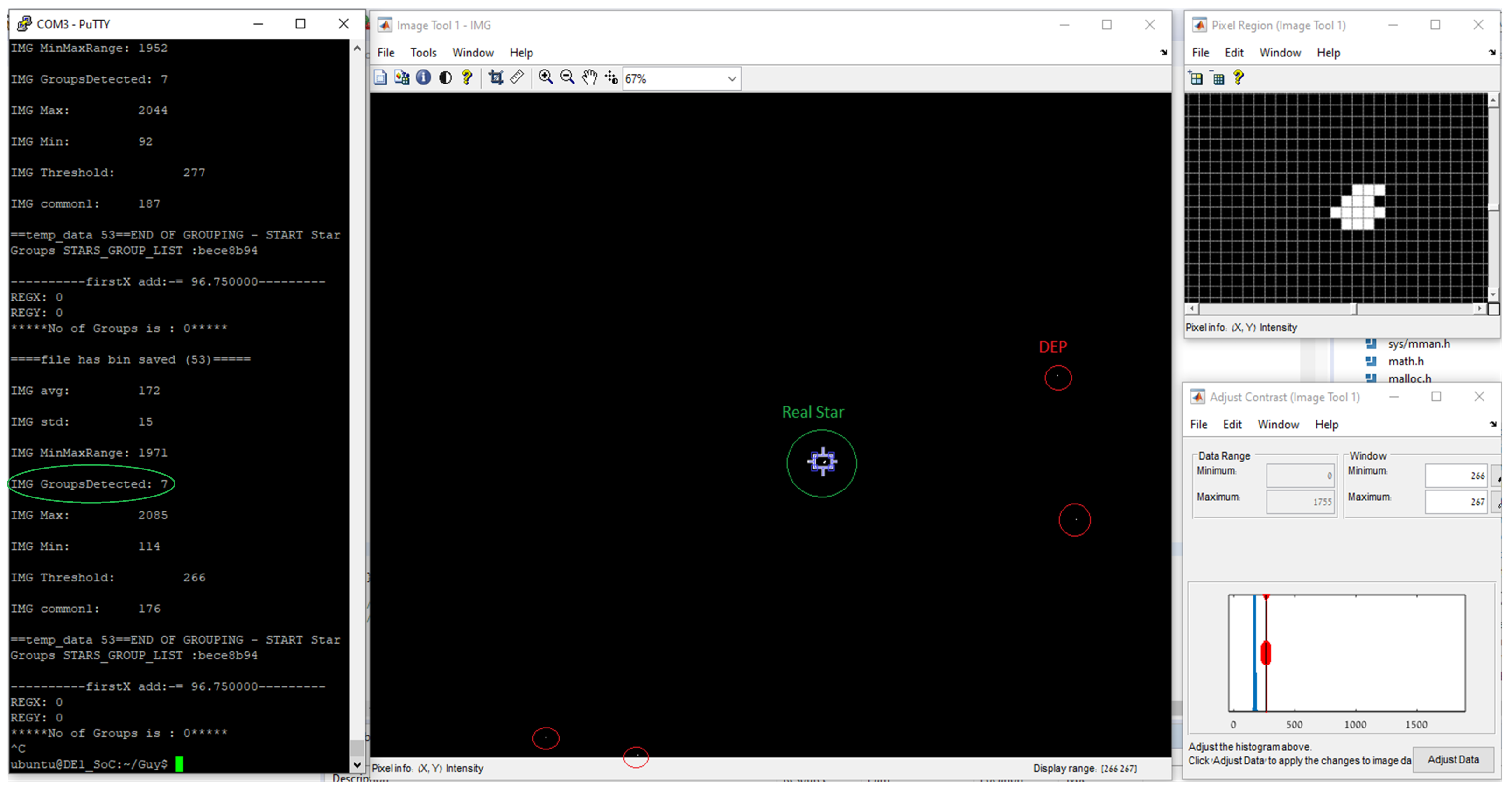
• A screen that displays the captured image at 60 FPS;
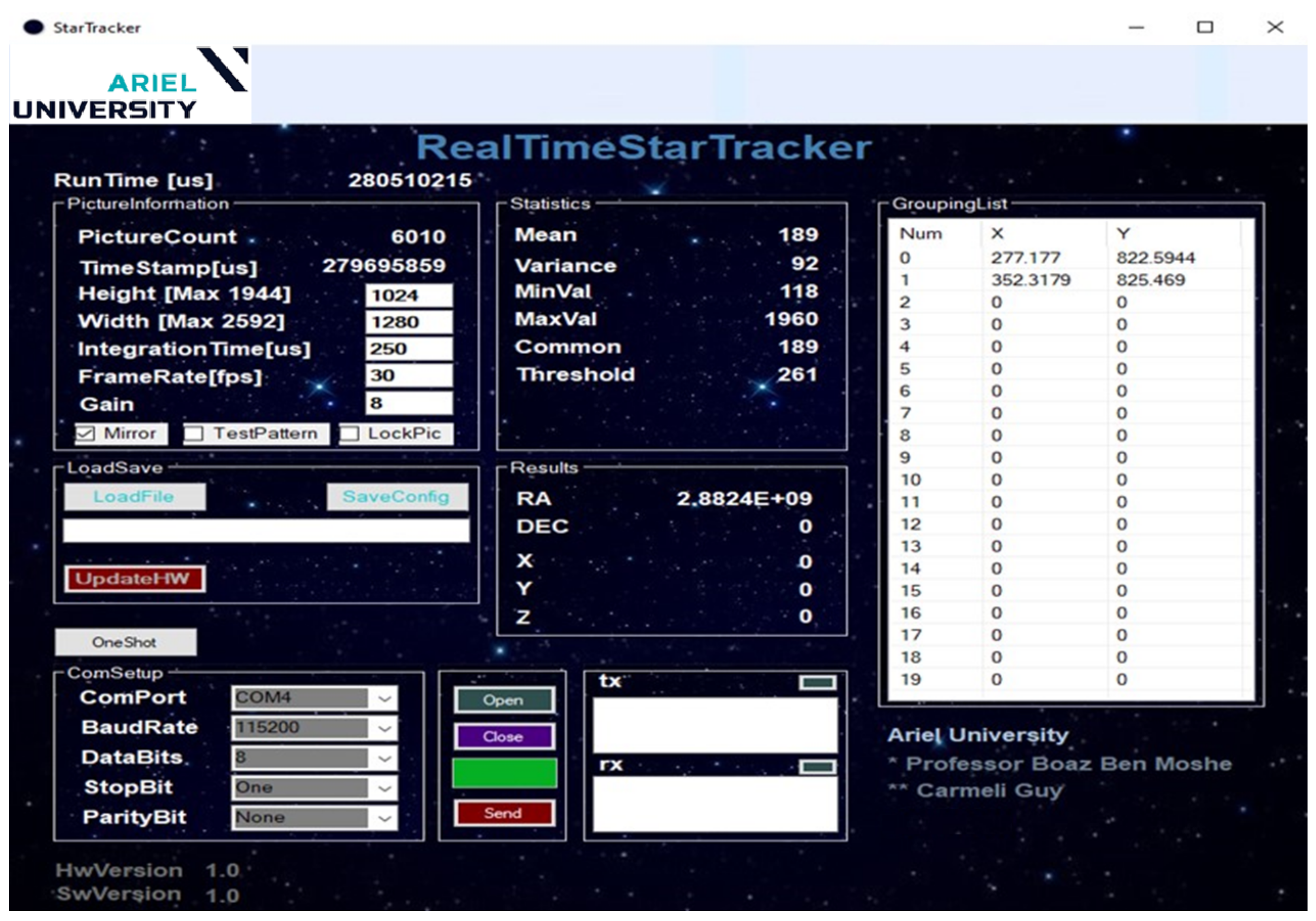
• A GUI application that allows a convenient interface with the camera for testing purposes during the study and for displaying the results after the image has been processed.

The FPGA serves as the central component of the system, performing hardware acceleration tasks for image processing. An on-chip Nios mini-processor assists by handling camera control tasks. Additionally, an on-chip ARM processor, running Ubuntu 16.0.04 OS, employs C and Python applications to enable communication with the FPGA hardware/logic, send and receive commands, perform a simple non-uniformity calibration (NUC) on the image, and execute the final “lost-in-space” algorithm against an Almanac. During image processing operations, the FPGA displays the image on the screen at a constant rate of 60 FPS, regardless of the input frame rate, with a resolution of 1280 × 1024 (Figure 2). The FPGA also interacts with the PC GUI and receives/sends image properties for analysis.

2.1. Optical Sensor and Image Capture

Selecting the right sensor for star research is critical and involves careful consideration of sensor properties relevant to practical experiments. For this reason, it is highly recommended to choose a high-quality camera that can produce images without clusters of defective pixels or “hot” pixels, which are commonly referred to as DEPs. These issues can significantly affect the accuracy and reliability of star observations, making it essential to select a sensor that is capable of producing high-quality data. Despite this requirement, it is worth noting that this study used a regular camera to demonstrate how the research idea can be integrated into low-cost systems without compromising accuracy or reliability. The Nios processor is responsible for controlling the optical sensor [14], initializing its registers, and managing critical parameters, such as exposure time, analog/digital gain, and resolution. Image capture can be triggered manually through a push button or by the processor itself. Once the camera captures the image, it sends a Bayer format image to the FPGA, which stamps the image with a time tag and converts it from Bayer [16] to RGB and then to YCbCr to obtain the intensity image Y. Meanwhile, a histogram and statistics, such as $\mu$, $\sigma$, Min/Max, Common1, Common2, Range & Saturation State, are calculated in parallel while the intensity image is transferred to the DDR memory. Thanks to the on-the-fly image transformation to RGB and Y, the image stream to the DDR memory experiences only a minor latency of a few hundred microseconds. In parallel to those operations, the RGB image is sent for display on the VGA screen at 60 FPS.

The sensor properties are described in

Table 1. Camera properties.

Subject	Parameters	Our Case
Active Matrix [mm]	5.7H × 4.28V 1	2.81H × 2.25V
Active pixels	2592H × 1944V	1280H × 1024V
Pixel size	2.2 × 2.2 $\mathsf{\mu }$m
Bit depth Global shutter	12 bit
Gain A/D	1–16 Analog, Digital	16 Analog
FOV [deg]	According to lens	13.38H × 10.72V

¹ V—Vertical, H—Horizontal.

.

With the Sunex DSL901J-NIR-F3.0 lens [17] with a 4 mm aperture, we obtain the information described in

Table 2. Single-pixel field of view.

Feature	Value
Sensor	MT9P001
Lens: SUNEX	DSL901j-NIR-F3.0
Focal length	12 mm
F#	3
Aperture	4 mm
SensorActiveArea-X	0.002816 m
SensorActiveArea-Y	0.0022528 m
X	1280 Pixels
Y	1024 Pixels
Pixel Size	2.2 $\mathsf{\mu }$m
Fov(x)	$2arctan\frac{0.5AactiveAreaX}{focallength}$ = $13.{38}^{\circ }$
Fov(Y)	$2arctan\frac{0.5AactiveAreaY}{focallength}$ = $10.{72}^{\circ }$
deg/Pixel(x)	$\frac{13.{38}^{\circ }}{1280\mathrm{pixels}}$ = 0.01045$\frac{deg}{\mathrm{pixels}}$
deg/Pixel(y)	$\frac{10.{72}^{\circ }}{1024\mathrm{pixels}}$ = 0.01046 $\frac{deg}{\mathrm{pixels}}$
deg/Pixel(avg)	$10.46\times {10}^{-3}\frac{deg}{\mathrm{pixels}}$

.

Finding the angular distance:

In the process of matching stars in a picture with a star map, we need to measure the distance between each two neighboring stars, which is often unknown and large. As a result, the angular distance is commonly used. An angular distance across the sky is defined as an angle between two-unit radius vectors from the center of a sky sphere pointing toward the two objects. This is also the shortest angular distance across the sphere between the two objects. In order to find the angular distance of two stars, we first need to define our system resolution, which is to know the angular distance spread by a single pixel (Table 2). Computationally, the angular distance d, between two celestial coordinates, can be calculated using the following formula: suppose that $\overrightarrow{a}$ and $\overrightarrow{b}$ are unit vectors representing a star direction vector, so $d=arcos(\overrightarrow{a}·{\overrightarrow{b}}^T)$. In our case, each pixel covers an angular distance of $10.46·{10}^{-3}$ degrees, so the angular resolution of our image is $10.46\times {10}^{-3}\frac{deg}{\mathrm{pixels}}$.

2.2. Image Processing

In general, all the high-computation operations are carried out by the FPGA. Camera triggering causes the sensor to expose the optical matrix in Global Shutter mode. The image transferred to FPGA for processing comes in a Bayer Pattern format (Figure 3). In most high-resolution sensors, the detector matrix is provided in this format, reducing the information transfer time and the amount of information flowing from the sensor to the image processor. During the image reconstruction process, the FPGA evaluates the two missing colors using the nearest neighbors algorithm, which is expressed in Equation (1):

$${\widehat{I}}_{(i,j)}=\left\{\begin{array}{l}(R_{(i,j)},{\widehat{G}}_{(i,j)},{\widehat{B}}_{(i,j)}),foriodd\&jeven\\ ({\widehat{R}}_{(i,j)},{\widehat{G}}_{(i,j)},B_{(i,j)}),forieven\&jodd\\ ({\widehat{R}}_{(i,j)},G_{(}i,j),{\widehat{B}}_{(i,j)}),otherwise\end{array}\right.$$

(1)

for example (relative to Figure 3):

At $R_{(3,4)}$ the two complementary colors B and G are obtained by Equation (2):

$$\begin{array}{c}\hfill {\widehat{B}}_{(3,4)}=0.25(B_{(2,3)}+B_{(2,5)}+B_{(4,3)}+B_{(4,5)})\\ \hfill {\widehat{G}}_{(3,4)}=0.25(G_{(3,3)}+G_{(2,4)}+G_{(3,5)}+G_{(4,4)})\end{array}$$

(2)

At $B_{(2,3)}$, the two complementary colors R and G are obtained by Equation (3):

$$\begin{array}{c}\hfill {\widehat{R}}_{(2,3)}=0.25(R_{(1,2)}+R_{(1,4)}+R_{(3,2)}+R_{(3,4)})\\ \hfill {\widehat{G}}_{(2,3)}=0.25(G_{(1,3)}+G_{(2,2)}+G_{(3,3)}+G_{(2,4)})\end{array}$$

(3)

At $G_{(2,2)}$ the two complementary colors R and B are obtained by Equation (4):

$$\begin{array}{c}\hfill {\widehat{R}}_{(2,2)}=0.5(R_{(1,2)}+R_{(3,2)})\\ \hfill {\widehat{B}}_{(2,2)}=0.5(B_{(2,1)}+B_{(2,3)})\end{array}$$

(4)

At $G_{(3,3)}$ the two complementary colors R and B are obtained by Equation (5):

$$\begin{array}{c}\hfill {\widehat{R}}_{(3,3)}=0.5(R_{(3,2)}+R_{(3,4)})\\ \hfill {\widehat{B}}_{(3,3)}=0.5(B_{(2,3)}+B_{(4,3)})\end{array}$$

(5)

The RGB image undergoes a linear transformation to YCbCr. The purpose of the transition is to obtain a Y component that describes the intensity of the brightness in the grayscale image. The statistics and histogram are extracted from the Y component as it is saved to memory. The FPGA performs the following calculations (see Equation (6)) as the information flows into memory:

• Image average, STD, and variance, which are used to calculate parameters for the thresholding process;
• Pixel min/max value, range: max–min, which can be used for image enhancement of the display, such as stretching the histogram of the image;
• Building a histogram and finding the parameters: common1, number of pixels in common1, common2, number of pixels in common2, saturation signal (actively high when 20% of the pixels are above 90% of brightness), and the number of pixels above the saturation value. The FPGA looks for two common values, one on the left side of the histogram for dark pictures and the other on the right side of the histogram for images with either the sun or the moon. The common value is used for the threshold calculation and for the exposure-time control mechanism. This process is performed on every single frame.

$$\begin{array}{c}\hfill {\sigma }^2=\left(\frac{1}{N}\sum _{n=1}^N{X}_i^2\right)-{\mu }^2,\mu =\frac{1}{N}\sum _{n=1}^N{X}_i\end{array}$$

(6)

After the intensity image Y, is saved into shared memory, the FPGA triggers the ARM processor to perform non-uniformity calibration (NUC) using a predefined “Dead Pixels” table. Once the NUC correction is completed, control is returned to the FPGA, which reads the NUC-updated image from memory and applies statistical threshold filtering, followed by cluster extraction. Finally, all image properties are internally saved and transferred to the GUI (Figure 4) for analysis.

2.2.1. Non-Uniformity Calibration and Statistical Thresholding

The automatic calibration of image sensor involves compensating for certain irregularities in the optical matrix. Specifically, the presence of dark pixels that are not part of the visible resolution requires a calculation of random noise that must be subtracted from the visible pixel value during image reading. Furthermore, defective pixel elements need to be repaired prior to threshold processing. In order to identify DEPs, we capture images under dark conditions or use a black body. Any pixels that deviate from the expected behavior of the detector matrix are identified and marked. The coordinates of these DEPs are mapped and substituted with a local/global common value in accordance with the ARM processor’s DEPs list. Although this procedure does not preclude the occurrence of random “hot” pixels, such single pixel events can be treated by the cluster detection algorithm. In Figure 5, we can see one star that does not belong to the DEPs list, marked in green, all others are known DEPs.

After performing the NUC, the processor initiates an image read request. The FPGA begins to read the image from the memory in order to extract the groups. Prior to the cluster detection process, the image goes through the statistical threshold analysis, where instead of $\mu$, we take the common value from the histogram. The threshold selection process is dynamic, with the threshold value in each image determined by the latest statistics of that image. The specific value, i.e., 250, used in Equation (8) (shown below) depends on the camera and its constant noise level:

$$\begin{array}{c}\hfill threshold=Common+3·\sigma +Bias\end{array}$$

(7)

$\forall Imag{e}_{invideostream}$

$$\begin{array}{c}\hfill Threshold=\left\{\begin{array}{c}250,ifThreshol{d}_i<250\hfill \\ \mathrm{T}\mathrm{h}\mathrm{r}\mathrm{e}\mathrm{s}\mathrm{h}\mathrm{o}\mathrm{l}\mathrm{d},ifThreshol{d}_i\ge 250\hfill \end{array}\right.\end{array}$$

(8)

$\forall Pixe{l}_{inimage}$

$$Pixe{l}_i=\left\{\begin{array}{c}0,ifPixe{l}_i<Threshold\hfill \\ Pixe{l}_i,ifPixe{l}_i\ge Threshold\hfill \end{array}\right.$$

(9)

2.2.2. Clustering Detection and Saving Groups to Memory

After the image passes the statistical threshold, a process of detecting a pixel group mass center is performed. This process is based on the fact that a star is relatively small, with a diameter of 9–11 pixels. The clusters detection algorithm operates as a raster line scanner (Figure 6). It scans the threshold-filtered image and identifies pixel clusters, each represented by their mass center x, y and their mass. Each such cluster is considered a single star (the algorithm is optimized for star detection, and thus, ignores large objects that have a diameter larger than 13 pixels, such as the moon and sun). Star properties are stored in the DDR memory in the following format: [∑ xiwi, ∑ wi, ∑ yiwi] (

Table 3. Group structure in DDR memory.

DDR addr	Base	++4h	++8h	++Ch	++10h
Variable	Total groups	${\sum }_{n=1}^N{X}_i{W}_i$	${\sum }_{n=1}^N{W}_i$	${\sum }_{n=1}^N{Y}_i{W}_i$	${\sum }_{n=1}^N{X}_i{W}_i$
Group No.	–	Group1	–	–	Group2

).

Line Scanner-Based Clustering Detection: How It Works:

During the line scan, the column vector is scanned using 13 pixels from 13 neighboring lines and the presence of a star is either confirmed or denied (Figure 6). If there is a non-zero value at the vector edges, then the star is rejected. When a potential star is identified, the FPGA records it in memory. The star’s shape is retained in the form of [$\sum x_i{w}_i$,$\sum w_i$,$\sum y_i{w}_i$] format. In this way, the values X, Y, and Magnitude can be later extracted by the ARM processor at a sub-pixel level (Equation (10)). Since the scanning process is performed continuously on the image, there may be duplicate stars in the resulting list. To address this, after the scanning is completed, the ARM sorts and filters the groups list based on the coordinates [X,Y] of the constellations. Finally, the groups without repetitions are sent to the “lost-in-space” algorithm, and at the same time, the data are sent to the GUI for presentation.

$$\begin{array}{c}\hfill Cy=\frac{{\sum }_{n=1}^N{Y}_i{W}_i}{{\sum }_{n=1}^N{W}_i};Cx=\frac{{\sum }_{n=1}^N{X}_i{W}_i}{{\sum }_{n=1}^N{W}_i}\end{array}$$

(10)

where N—number of pixels in group, i—pixel Index (at x or y direction), $W_i$—pixel value at index i.

2.3. Star Pattern Recognition Related to Almanac

After clustering detection is completed, the FPGA sends a command to the ARM processor to begin executing the lost-in-space algorithm. The processor then reads the clusters data from memory, calculating the coordinates and magnitudes of each suspected star in the image and then performs filtering, to filter out repetitive stars. The list of coordinates for the five stars is sent to both the self-organizing map neural network for further processing and to the graphical user interface (GUI) for display purposes. The “lost in space” algorithm, described in Figure 7, option 2, demonstrates how pattern recognition is performed by matching coordinate series obtained from the camera against the star map. For each star, four neighboring stars are selected based on camera sensitivity within a given field of view (FOV). For this study, a $[{15}^{\circ }X,{15}^{\circ }Y]$ FOV was taken and the database was built using a four-neighboring-star basis with a pixel contribution of 10.41 millidegrees per pixel.

The neural network architecture of SOMs consists of an input layer and an output layer. The input layer is also called the features vector, which receives the high-dimensional input data, and the output layer contains a set of neurons organized in a grid-like structure. Each neuron in the output layer represents a different cluster or group. During training, the weights of the output layer neurons are adjusted to map the high-dimensional input data onto the lower-dimensional output layer grid. This process results in a 2D representation of the input data, which can be visualized as a map or a scatter plot. To generate this feature vector (Algorithm 1), we begin by selecting the five strongest stars from the list of stars. We determine the strength of each star based on its brightness criteria. Next, we identify the star closest to the center of the image matrix and designate it as the main star. From these selected stars, we generate a feature vector containing ten angular distances that are sorted in ascending order. To calculate the angular distances, we measure the angle between the main star and each of the other four stars, as well as the angles between each pair of the four stars themselves. This feature vector is then used as input for the SOM network to perform pattern matching or clustering.

Algorithm 1 ARM preparatory actions for pattern matching using an AI Kohonen map [1]

1: Sort all the stars in the image from the strongest to the weakest and selecting the five strongest stars (Figure 8). 2: Mark the star closest to the center as the main star. 3: The other four neighboring stars are selected so that they are within a radius equivalent to the distance of $Rt<R<R_{FOV}$ (Rt = 0.5 to 1.0 degrees, $0.85<R<7.5de{g}_{max}$ in our case) from the main star. The selected stars are arranged by their distance from the main star, closest to furthest. 4: Looking at the distances between any two stars in a five-star group $\left(\genfrac{}{}{0pt}{}{5stars}{2distances}\right)=\left(\genfrac{}{}{0pt}{}{5}{2}\right)=10distances$, we gather all 10 distance combinations (Equations (11) and (12)). Neighbors are selected in such a way that they cannot be closer than 20 pixels in angular distance to another star [1]. 5: The angular distances are sorted in ascending order and constitute the features vector.

$$\begin{array}{c}\hfill FeatureVector:Ptr=\left[r_1^T{r}_2{r}_1^T{r}_3{r}_1^T{r}_4{r}_1^T{r}_5{r}_2^T{r}_3{r}_2^T{r}_4{r}_2^T{r}_5{r}_3^T{r}_4{r}_3^T{r}_5{r}_4^T{r}_5\right]\end{array}$$

(11)

$$\forall Star:r_i=[\frac{x_i}{\sqrt{x_i^2+y_i^2+f^2}}+\frac{y_i}{\sqrt{x_i^2+y_i^2+f^2}}+\frac{f}{\sqrt{x_i^2+y_i^2+f^2}}{]}^T$$

(12)

where $r_i$—direction unit vector, $(x_i,y_i)$—star coordinates. f—focal length.

Figure 8. Camera FOV: star number is arranged by intensity.

Figure 8. Camera FOV: star number is arranged by intensity.

Once we calculated the feature vector, we introduce the features vector to the well-trained Kohonen network (Figure 9) and obtain an index by which we can return to the star map and find the appropriate direction vector—line of sight. There are many ways to think about how the database is organized, and it is possible to characterize it, build the features vector accordingly, run it, and test whether the results are satisfactory.

2.3.1. Building the Database Using Camera Sensitivity in a Given FOV, for NN Training

To train the network using the Almanac stars list, we need to filter out stars that cannot be detected by the specific camera due to its sensitivity. Once we have a list of candidate stars, we create a corresponding feature vector for each star based on the neighboring stars within a given field of view (FOV) as follows:

1.

Select the radius in a FOV; in our case, radius R = 7.5 deg.

2.

From the Tycho2 2018 almanac, a sensitivity of magnitude 6 is selected. The database is filtered accordingly and then sorted by intensity from high to low. The map is now reduced to 4642 stars out of over two million.

3.

For each star, we take the four brightest neighboring stars, for which the minimum distance between the main star and the nearest neighbor is 0.85 degrees.

4.

Find the distances between any two stars in a five-star group. We gather all 10 distance combinations. Neighbors are chosen in such way that they are not closer than 20 pixels (angular distance) to another star.

5.

The angular distances are sorted in ascending order and constitute the features vector of the SOM.

We now create the list shown in

Table 4. An ordered database of stellar distances.

MainStar Index	Feature1	Fea.2	Fea.3	Fea.4	Fea.5	Fea.6	Fea.7	Fea.8	Fea.9	Feature10
1	0.4423	0.5401	0.5713	1.7155	2.2265	2.2459	2.3442	3.5961	3.9351	4.1632
2	1.1573	1.6522	2.0266	2.4743	2.7054	2.7343	4.0751	4.3159	5.1978	6.5945
3	0.169	1.269	2.5161	2.7003	2.866	3.2137	4.6179	4.7815	5.658	5.8259
4	0.1473	0.9652	1.7718	1.836	1.9854	2.5176	2.8021	2.8488	3.6899	3.719
…	…	…	…	…	…	…	…	…	…	…
4642	2.6456	4.3696	6.0897	6.2987	6.6346	6.7552	7.0136	7.8045	9.025	12.6147

.

Visually, in Figure 10, we can see an example of a sky ball with neighboring stars at the defined spatial angle of 7.5 deg.

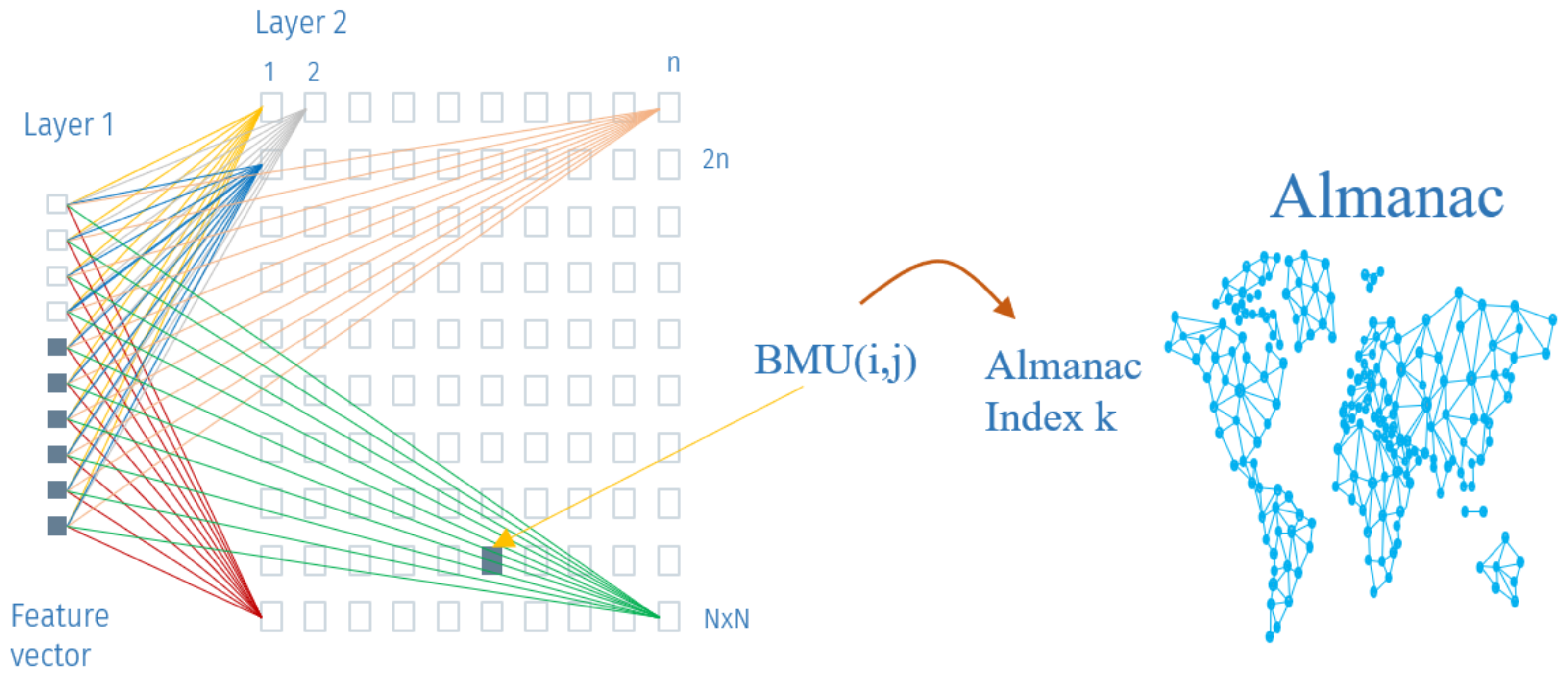
2.3.2. Building a Self-Organizing Map Network—Kohonen Map

There are a number of topologies for building the network, the map structure, and the distances from neighboring neurons (e.g., triangle, bubble, Mexican hat, Gaussian, hexagon). During the research, Gaussian topology was used in the SOM structure and the MiniSom library in Python was used.

Network structure:

• Size: 69 × 69;
• Features vector: 10;
• Clusters output: 4642;
• Sigma: 3;
• Learning rate: 0.7;
• Neighborhood function: Gaussian;
• Train batch: 1 M.

When the network is ready, we pass the entire database through the network and commence training. For each feature, the weight network wij is updated until, finally, we obtain a distance map that describes the distance distribution (Euclidean distance $\parallel x-w_{ij}\parallel$) between the neighbors. For each pattern in the dataset, the corresponding winning neuron has been marked. Each type of marker represents a main star class. If the average distance is high, then the surrounding weights are different and the color is bright; if the average distance is low, then a dark color is applied, as described in the following image (Figure 11).

The algorithm works such that for a given cluster, the best matching unit (BMU) neuron closest to 0 lights up. Furthermore, the environment around the winning neuron is the most supportive (Algorithm 2). The algorithm considers neighbor values using the activation frequency parameter. This parameter is based on the relative frequency at which each neuron is contained in the neighboring BMU, so that there is an individual memory of activation obtained from each neuron (a realistic characteristic that changes the dynamics of map formation). Using this parameter reduces the network error. In the following image (Figure 12), we can see the activation frequency map of our application.  

Algorithm 2 Apply the self organizing map (SOM) algorithm: repeat the following procedure until the map converges1.

At each time t, present an input$X_{\left(t\right)}$and select the winning neuron ${\nu }_t=arg$$\begin{array}{c}\underset{k\in \mathsf{\Omega }}{min}\end{array}$$\parallel X_{\left(t\right)}-w_{K\left(t\right)}\parallel$ Update the weights of the winner and its neighbors $\mathsf{\Delta }{w}_{k\left(t\right)}={\alpha }_{\left(t\right)}{\eta }_{(\nu ,k,t)}[X_{\left(t\right)}-w_{\nu \left(t\right)}]$ ${\eta }_{(\nu ,k,t)}=e^{-\frac{\parallel r_{\nu }-r_k\parallel }{2{\sigma }_t^2}}$

1 whereby: $X\in R^n$ is the input vector; At the start of the learning process, all the weights $\{w_1,w_2,\dots ,w_M\}$ are initialized to small random numbers; $w_i$ is the weight vector associated with neuron i and is a vector of the same dimension n of the input; $r_i$ is the location vector of neuron i on the grid (M is the total number of neurons on the grid); ${\alpha }_{\left(t\right)}$ has a learning rate of rate (0,1) and the scalar decreases monotonically; ${\sigma }_{\left(t\right)}$ represents the effective range of the neighborhood and often decreases with time; ${\eta }_{(v,k,t)}$ is the neighborhood function, $\nu$ is the winning neuron, and k is the neighbor neuron; $\mathsf{\Omega }$ is the set of neuron indexes.

At the same time, we look at two trends that provide information about network convergence: quantization error and topographic error (Figure 13). Results with a confidence of 97.7% were achieved in the training process. The quantization error refers to the average distance between the input data and the best-matching neuron in the SOM. It is a measure of how well the SOM has grouped similar input data together into clusters, and can be used to assess the quality of the map’s representation of the input data. Topographic error, on the other hand, refers to the proportion of neighboring neurons in the SOM that are not topologically adjacent to the best-matching neuron for a given input data point. In other words, it measures how accurately the SOM has preserved the topology of the input data in the map. A lower topographic error indicates that the SOM has accurately mapped similar input data to nearby neurons in the map.

The product we obtain from the network is a labels map that links the star index to the mapping (i, j) in the Kohonen map. When the network is well trained, for each entry Vector-K entering the network, the suitable neuron in position (i, j) will be obtained. In case where looking up a vector yields multiple possible solutions, the algorithm can be re-run with a different main star at each time. At the end of the process, the MainStar index is located and the LOS can be found.

3. Results

After an overview of the study, the current focus shifts to the presentation of the results specifically related to stars pattern recognition. With the neural network trained to recognize star patterns using feature vectors, the following example was examined:

Suppose $\overrightarrow{V_1}$ is the input vector corresponding to a star in index 21 and its neighbors N1-N4 are taken from the Almanac as described in

Table 5. An example of a structure of five neighboring stars.

Main Star Index	N1	N2	N3	N4 1
21	423	449	446	70

¹$N_i$ is the matching neighbors’ indexes.

.

${\overrightarrow{V}}_{(i=21)}$ [0.4556 , −0.5362 , −0.7106].

The feature vector of a star index 21 (

Table 6. Star index 21, angular distances [deg].

Star Index 21 Feature Vector [0–9]
3.1083	4.3947	5.0128	5.0412	6.1340	6.6687	6.6815	8.7224	9.4316	9.6025

) is taken and random noise is added to it of up to four pixels, to simulate the stars sampled from the sky image.

When searching for a solution over the network, we obtain the Kohonen index (48, 51) and the corresponding Star index ({`21’: 1}). The solution is identified with a confidence level of 97.7% as being associated with the Star index 21. In this case, we can stop the search and the LOS can be found by adding or subtract the angle of the star from the center of the detector. The result is achieved in about 870 us.

Additional checks can be performed, e.g., the next neighbor N1, Star 423, can be taken as the main star and the feature vector can be created (see

Table 7. Changing the main star, obtaining five new neighboring stars.

Main Star Index	N1	N2	N3	N4 1
423	449	21	539	373

¹ Neighboring star.

and

Table 8. Star index 423, angular distances [deg].

Star Index 423 Feature Vector [0–9]
3.1083	4.3947	4.6086	5.0128	5.4160	6.1670	8.0109	8.3438	9.2132	9.5359

).

As we can see, it requires two additional stars in the image, i.e., N3 and N4. The Kohonen result for this input is three possible options: Kohonen Index (36, 47) and Star Index ({`423’: 1, `1822’: 1, `3125’: 1}). For a particular five-star structure, there is more than one option. The more stars there are in the picture, the less likely the pattern will be the same. From the last check, main star index 21 was marked as $\overrightarrow{V_1}$, and stars index 423, 1822, and 3125 as $\overrightarrow{V_2}$, $\overrightarrow{V_3}$, and $\overrightarrow{V_4}$, respectively, while ($\overrightarrow{V_i}$) is the unity vector represented by $[x,y,z]$ vector from the database:

$$\begin{array}{c}\overrightarrow{V_1}=[0.4556,-0.5362,0.7106]\\ \overrightarrow{V_2}=[0.5201,-0.4982,0.6938]\\ \overrightarrow{V_3}=[-0.2666,-0.8688,0.4172]\\ \overrightarrow{V_4}=[-0.0745,-0.4937,0.8664]\end{array}$$

(13)

Testing the results by constraint on the following equation:

$$\begin{array}{c}\hfill 7.5\left[\mathrm{deg}\right]\ge arccos(\overrightarrow{V_1}·{\overrightarrow{V_i}}^T)\end{array}$$

(14)

shows that:

$$\begin{array}{c}{\theta }_1=arccos(\overrightarrow{V_1}·{\overrightarrow{V_2}}^T)={4.39}^{\circ }\\ {\theta }_2=arccos(\overrightarrow{V_1}·{\overrightarrow{V_3}}^T)={50.149}^{\circ }\\ {\theta }_3=arccos(\overrightarrow{V_1}·{\overrightarrow{V_4}}^T)={32.17}^{\circ }\end{array}$$

(15)

From the database structure, we know that neighboring stars are within a 7.5 deg radius; thus, ${\theta }_2$ and ${\theta }_3$ are rejected and the result is star index 423: $\overrightarrow{V_2}$ = [0.5201 , −0.4982 , 0.6938].

4. Timing and Performance

The performance of star identification algorithms is typically evaluated based on two key indicators: identification time and memory consumption. The algorithm proposed in this study was implemented on a Cyclone V SoC FPGA and achieved the timing performance described in

Table 9. System timing.

Feature	Performance 1
Exposure time	Varies as needed 100 ms to 500 ms. Camera dependent
Reading the image from the sensor (3 × 12 bit), Performing image processing and memory retention	∼14 ms (Read image from sensor takes 13.6 ms Clk = 96 Mhz, Resolution 1280 × 1024)
Bayer To RGB-YCbC	latency 166 us: done on the fly
Building a histogram & collecting statistics	0 delay, done on the fly, in parallel.
Nuc—Clear DEPs	78 us , Done by HPS processor
Threshold and Clusters Detection, save groups to MeM	∼14 ms (reading image from memory takes 13.1 ms, Clk = 100 Mzh, resolution 1280 × 1024)
AI Neural Network result	870 us

¹ Can achieve 2 ms End2End, from image request to LOS vector results.

. The platform’s end-to-end runtime is 27.64 ms, from the image request to the Line of Sight (LOS) results, with most of the time spent on reading data from both the sensor and DDR memory.

Table 10. Comparison of identification time and memory consumption.

Algorithm Identification	Time	Memory Consumption
Proposed algorithm	870 us	249 KB
NN Based algorithm [6]	32.7 ms	1920.6 KB
Pyramid algorithm [19]	341.2 ms	2282.3 KB
Optimized Grid algorithm [20]	178.7 ms	348.1 KB
Modified LPT algorithm [21]	65.4 ms	313.5 KB

presents the average identification time and memory consumption for several algorithms [6] (such as “Robust Star Identification Algorithm Based on Neural Networks” [6], Optimized Grid algorithm [18], etc.) running on a computer. The results show that the proposed algorithm has a significantly shorter identification time compared to other algorithms, with the self-organizing map (SOM) runtime being approximately 870 microseconds. Additionally, using image sensors with high-speed MIPI or LVDS interface can further reduce the read time to less than 1 millisecond. By leveraging statistics from previous images, a total processing time of about 2 milliseconds End2End can be achieved from the image request command to the LOS vector result, with some compromises. Moreover, the proposed algorithm requires only 249 KB of memory, which is smaller than the other algorithms.

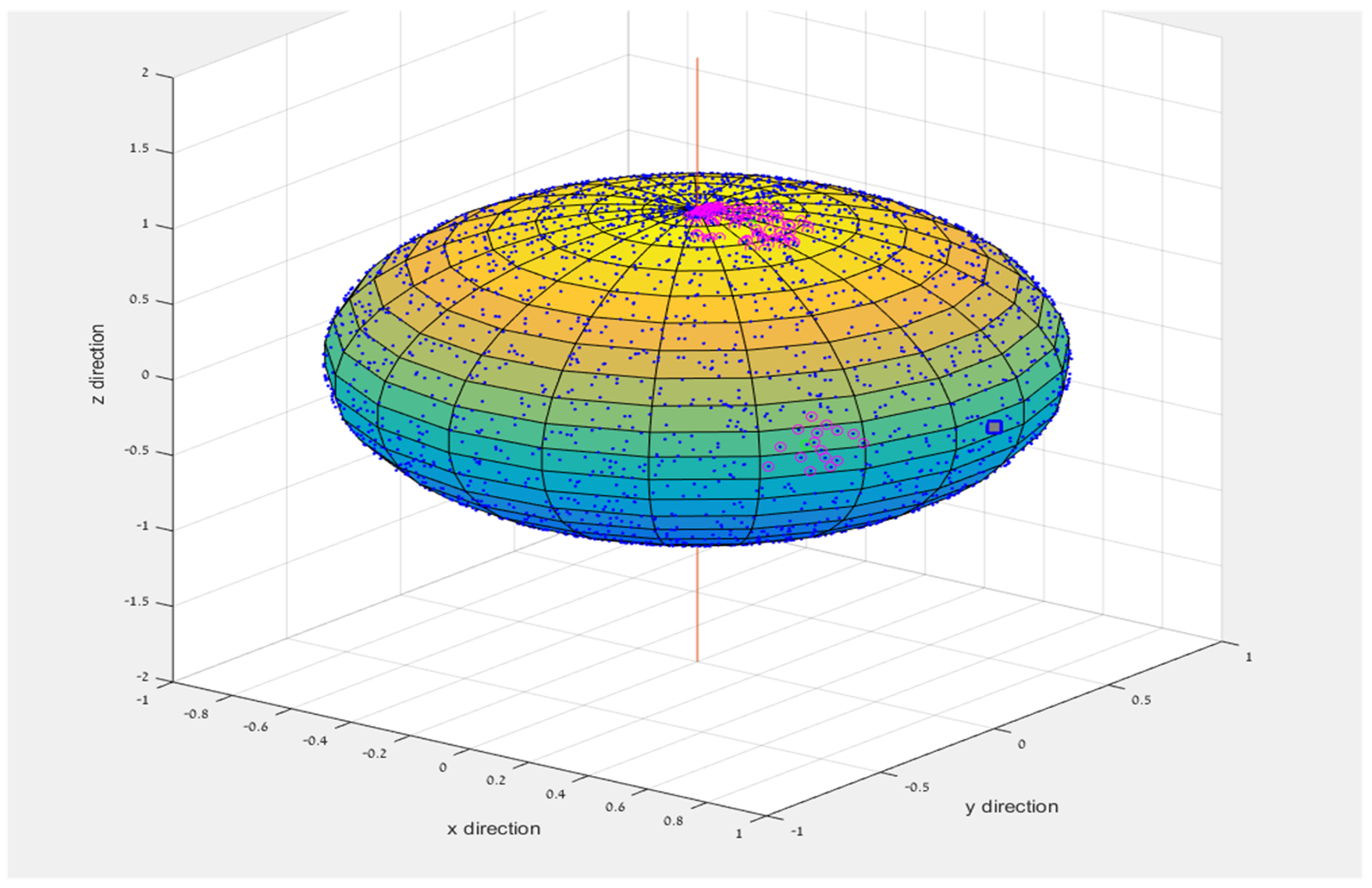
Expected Pointing Accuracy

In this subsection, we discuss the expected accuracy of the presented star tracker system—assuming the identification of the stars was performed properly.

The camera used for the presented star tracking system has an angular field of view of about $0.01$ degree per pixel (as shown in Table 2). As a rule of thumb, one may assume that the expected accuracy is on a pixel scale (say 0.01 degree). This is often the case when a naive star coordinate is used (without any super-resolution). In the experiments conducted, an error margin of ±4 pixels were used for the star position. However, once we determine the star index we are pointing at, we can promptly mark the main star. The accuracy primarily relies on the influence of the lens on the pixel FOV error and the correction of the spread resulting from movement. The actual pointing accuracy depends on the number of identified stars in the image and their location in the frame (which affects the pointing errors related to lens imperfection calibration). As an overall conclusion, the presented star-tracking framework was able to achieve a pointing accuracy better than two pixels in most tested cases. Such accuracy (about 0.019 degrees, or about 0.33 milliradian) is sufficient for low-resolution imaging and laser pointing applications. Improved accuracy may be achieved by using “super-resolution”; recall that we compute the angular distance in a sub-pixel calculation on the center of mass of the stars. Thus, an angular error on a sub-pixel scale should be achievable. Moreover, by using a well-calibrated lens system, the overall accuracy of the presented framework may allow sub-pixel accuracy even in single-star image cases (“lost in space” scenarios).

5. Discussion and Conclusions

The major emphasis in the above work is on the use of self-organizing map and on the ability to simplify the solution search, compared to other methods of pattern recognition. The research shows a high-speed result with a confidence of about 98% in the star pattern identification. The high confidence value does not guarantee that for each feature vector entry, a single solution is obtained; this is due to the fact that there may be different clusters with similar feature vectors. After obtaining the Kohonen match, it is good practice to make some logical test to understand the relation between the results. FPGA technology enables parallel processing across different design levels. This allows for efficient image processing with multiple processors, displaying images on a monitor at a high frame rate of 60 fps, and seamless communication with the GUI. Additionally, the use of different camera interfaces, such as LVDS, can significantly reduce sensor readout time to just a few milliseconds. By increasing the clock rate, the threshold and cluster extraction process can be shortened by half or more, leading to faster processing times. The real-time star tracker can be embedded as IP in existing hardware that contains FPGA and a camera, making it suitable for integration into nanosatellites being built by the university. Future work plans involve integrating convolutional neural networks (ConvNets) with landmark properties to further enhance the system’s performance.

References

1. Zhang, G.; Zhang, G. Star Identification Utilizing Neural Networks; Springer: Berlin/Heidelberg, Germany, 2017. [Google Scholar]
2. Gose, E.; Johnsonbaugh, R.; Jost, S. Pattern Recognition and Image Analysis; Prentice-Hall, Inc.: Hoboken, NJ, USA, 1996. [Google Scholar]
3. Mantas, J. Methodologies in pattern recognition and image analysis—A brief survey. Pattern Recognit. 1987, 20, 1–6. [Google Scholar] [CrossRef]
4. Salomon, P.M.; Glavich, T.A. Image signal processing in sub-pixel accuracy star trackers. In Proceedings of the 24th Annual Technical Symposium, San Diego, CA, USA, 29 July–1 August 1980; Volume 252, pp. 64–74. [Google Scholar]
5. Liebe, C.C. Accuracy performance of star trackers-a tutorial. IEEE Trans. Aerosp. Electron. Syst. 2002, 38, 587–599. [Google Scholar] [CrossRef]
6. Wang, B.; Wang, H.; Jin, Z. An Efficient and Robust Star Identification Algorithm Based on Neural Networks. Sensors 2021, 21, 7686. [Google Scholar] [CrossRef]
7. Xu, J.; Zhao, T.; Feng, G.; Ni, M.; Ou, S. A fuzzy C-means clustering algorithm based on spatial context model for image segmentation. Int. J. Fuzzy Syst. 2021, 23, 816–832. [Google Scholar] [CrossRef]
8. Kohonen, T. The self-organizing map. Proc. IEEE 1990, 78, 1464–1480. [Google Scholar] [CrossRef]
9. Vesanto, J.; Alhoniemi, E. Clustering of the self-organizing map. IEEE Trans. Neural Netw. 2000, 11, 586–600. [Google Scholar] [CrossRef] [PubMed]
10. Terasic. DE1-SoC Development Kit User Manual; DE1-SoC Manual; Terasic: Hsinchu, Taiwan, 2016. [Google Scholar]
11. Rockett, L.; Patel, D.; Danziger, S.; Cronquist, B.; Wang, J. Radiation hardened FPGA technology for space applications. In Proceedings of the 2007 IEEE Aerospace Conference, Big Sky, Montana, 3–10 March 2007; pp. 1–7. [Google Scholar]
12. Wirthlin, M. High-reliability FPGA-based systems: Space, high-energy physics, and beyond. Proc. IEEE 2015, 103, 379–389. [Google Scholar] [CrossRef]
13. Anjankar, S.C.; Kolte, M.T.; Pund, A.; Kolte, P.; Kumar, A.; Mankar, P.; Ambhore, K. FPGA based multiple fault tolerant and recoverable technique using triple modular redundancy (FRTMR). Procedia Comput. Sci. 2016, 79, 827–834. [Google Scholar] [CrossRef]
14. Terasic. Terasic TRDB D5M, 5 Mega Pixel Digital Camera Development Kit; USer Manual; Terasic: Hsinchu, Taiwan, 2017. [Google Scholar]
15. Support Intel. Intel SoC FPGA Embedded Development Suite User Guide; ug-1137; Support Intel: Santa Clara, CA, USA, 2019. [Google Scholar]
16. Minervini, M.; Rusu, C.; Tsaftaris, S.A. Computationally efficient data and application driven color transforms for the compression and enhancement of images and video. In Color Image and Video Enhancement; Springer International Publishing: Cham, Switzerland, 2015; pp. 371–393. [Google Scholar]
17. Sunex. Lens—Sunex DSL901j-NIR-F3.0. 2017. Available online: http://www.optics-online.com/OOL/DSL/DSL901.PDF (accessed on 4 April 2023).
18. Padgett, C.; Kreutz-Delgado, K. A grid algorithm for autonomous star identification. IEEE Trans. Aerosp. Electron. Syst. 1997, 33, 202–213. [Google Scholar] [CrossRef]
19. Mortari, D.; Samaan, M.A.; Bruccoleri, C.; Junkins, J.L. The pyramid star identification technique. Navigation 2004, 51, 171–183. [Google Scholar] [CrossRef]
20. Aghaei, M.; Moghaddam, H.A. Grid star identification improvement using optimization approaches. IEEE Trans. Aerosp. Electron. Syst. 2016, 52, 2080–2090. [Google Scholar] [CrossRef]
21. Luo, L.Y.; Xu, L.P.; Zhang, H.; Sun, J.R. Improved autonomous star identification algorithm. Chin. Phys. B 2015, 24, 064202. [Google Scholar] [CrossRef]
Figure 1. AI-based real-time star tracker system diagram.
Electronics 12 02084 g001
Figure 2. FPGA AI-based star tracker block diagram.
Electronics 12 02084 g002
Figure 3. Bayer pattern.
Electronics 12 02084 g003
Figure 4. Star Tracker GUI.
Electronics 12 02084 g004
Figure 5. Star detection report. On the left side of the report, we can see the Linux terminal output. It shows that the system detected one group seven times. This effect is due to the star search algorithm. After filtering out identical results, we are left with a single star. In the center of the image, we see star detection and DEP identification. In the top right corner, we see a reference image of a real star. Below it, there is an image histogram.
Electronics 12 02084 g005
Figure 6. Star detection by the FPGA.
Electronics 12 02084 g006
Figure 7. Star Identification algorithm: choosing stars by intensity.
Electronics 12 02084 g007
Figure 9. Kohonen map and indexing to Almanac.
Electronics 12 02084 g009
Figure 10. Neighboring stars at the defined spatial angle of R ≤ 7.5 deg.
Electronics 12 02084 g010
Figure 11. Kohonen distance map.
Electronics 12 02084 g011
Figure 12. Activation frequency map.
Electronics 12 02084 g012
Figure 13. Quantization error and topographic error. Quantization error: 0.00014; topographic error: 0.02218.
Electronics 12 02084 g013