Event-Triggered Adaptive Control for a Class of Nonlinear Systems with Dead-Zone Input

Abstract

In this paper, the event-triggered control problem is investigated using backstepping techniques for nonlinear systems with dead-zone input. The external disturbance and unknown parameters are also considered in the controller’s design. It is well known that errors in input signal measurements are inevitable. In event-triggered control, such errors will directly affect whether the control signal is updated. This measurement error can be seen in the form of interference to the threshold. Therefore, unlike traditional event-triggered control, the existence of threshold disturbance is considered in the controller’s design. The proposed controller can not only compensate for the uncertainties caused by external disturbance and unknown parameters but can also suppress the unknown effects caused by threshold interference. In addition, to obtain a continuous controller, a smooth function is constructed to approximate the discontinuous sign function. In this way, Zeno behavior is successfully avoided. The boundedness of all signals and the tracking performance of the system can be guaranteed by the proposed control scheme. Numerical simulation and actual system simulation demonstrate the effectiveness of the proposed control scheme. The comparative simulation results also verify this event-triggered controller’s advantages, including better tracking performance and fewer trigger times.

1. Introduction

In classical sample-data control, the output of the controller is continuously applied to the system at any time instant, although such continuous changes in the control input signal are sometimes unnecessary. This leads to a waste of system resources, including bandwidth and energy. In order to overcome these drawbacks, an event-triggered control strategy is proposed. The main idea is to determine whether the signal is updated based on system requirements and perform updates through the design of a triggering mechanism. Obviously, in order to achieve good system performance, the triggering mechanism and the design of the control inputs based on the triggering mechanism are the key issues. This requires us to fully consider the practical characteristics of the system actuators and all sorts of uncertainties when designing the event-triggered controller.

Dead zones, as nonlinear characteristics of the actuator, often exist in actual controlled systems. Ignoring their impact will inevitably hinder system performance. Therefore, many researchers have studied the control problem of systems with dead-zone actuators, and many results have been obtained. An adaptive control scheme was proposed for strict feedback systems with dead-zone input using backstepping techniques in [1]. By constructing observers to estimate the system states, an output feedback adaptive controller was developed in [2]. In this paper, a smooth inverse of dead-zone nonlinearity was constructed, and the design of this output feedback adaptive control law was applied. An output feedback learning control scheme using a neural network for nonlinear strict feedback systems with dead-zone input was proposed in [3]. Prescribed performance can be achieved by this proposed learning control scheme. Finite-time control techniques have also been implemented in the controller design for systems with dead-zone input, and several results were proposed in [4,5]. In addition, fault-tolerant control, global practical tracking, decentralized adaptive control, and sliding mode control have also been applied to uncertain systems with dead-zone input [6,7,8].

In view of the development of event-triggered control, the results for nonlinear systems are still very limited. In the last decade, event-triggered control for strict feedback systems has gradually gained attention from researchers. Backstepping technology [1,9,10,11,12,13], as a recursive design method, can effectively reduce the difficulty of controller design. It has been successfully applied to the event-triggered control of nonlinear systems [14,15,16,17]. In [14], event-triggered adaptive controllers based on the fixed threshold and relative threshold were developed. A threshold switching strategy was proposed by combining the advantages of fixed thresholds and relative thresholds. This strategy was applied to a class of nonlinear systems with unknown actuator failures [15]. For some or all states that cannot be measured, an output feedback event-triggered control law was proposed in [16]. The above results are only applicable for single nonlinear systems. For interconnected systems composed of multiple subsystems, [17] provided a design method for a decentralized event-triggered control scheme. In practice, dead zones [18,19,20,21,22,23,24,25] are a common non-linear limitation of input and output signals. Therefore, considering the limitations of dead-zone input in the design of event-triggered controller has practical significance [18,19,20,21,22]. An event-triggered adaptive control scheme was developed for a class of nonstrict-feedback nonlinear systems with dead-zone input in [18]. A fuzzy logic system was constructed to approximate unknown nonlinear functions, and to reduce repeated differentiation, dynamic surface control and backstepping technology were applied in the design of the input signal and update laws of unknown parameters. In [19], the event-triggered adaptive control problem was studied for a class of nonlinear systems with dead-zone input and external disturbance. The linear term of the estimated variables with a time-varying factor was introduced in the update law. Thus, a new update law was constructed. As an important issue in the field, the finite-time control problem for nonlinear systems with a dead-zone constraint and event-triggered input was also studied. In [21], the event-triggered finite-time control problem was addressed for a class of nonlinear systems with unknown dead-zone input. A neural network observer was constructed, and a tracking control scheme was proposed. In [22], an event-triggered control scheme was developed for nonlinear multi-agent systems with dead-zone input. The consistent tracking performance of controlled systems within a fixed time can be achieved using this proposed controller. Looking at the above results on the event-triggered control of nonlinear systems with dead-zone input, there are some problems that need to be addressed. One important issue is that the inevitable measurement errors in input signals were not taken into account. Such errors will lead to unknown interference on the threshold [18,19,20,21,22]. In [19,22], the upper and lower bounds of the unknown parameters in the dead-zone model must be known. In [18,21], the system model is relatively simple and does not consider the existence of unknown parameters in the system. In addition, Ref. [18], only provides results concerning semi-global uniform ultimate boundedness.

In this paper, we address event-triggered-based control design for a class of uncertain nonlinear systems with unknown parameters, external disturbance, and unknown dead-zone input. The key to the formation of the triggering mechanism lies in the construction of the triggering threshold. Considering the ubiquity of external interference, unknown interference terms were introduced in the threshold. A relatively dynamic threshold was thus constructed. The defining characteristic of this relative dynamic threshold is its mainly static constant values, supplemented by dynamic disturbances. In the controller design, the dead-zone transformation of the original signal and its triggered signal was analyzed. We proved that the error between the two signals after dead-zone transformation is bounded and provided detailed bounds. Then, we eliminated the uncertainty caused by all unknown disturbances by comprehensively estimating the upper bound of the system disturbance, threshold disturbance, and dead-zone transformation disturbance. At the same time, the uncertain parameters of the system and the unknown constant parameters in the dead-zone were estimated. In particular, in order to ensure the continuity of the control input signal, an approximate function of the $sign(·)$ function was constructed and used as a substitute for $sign(·)$ functions in the controller design. With the proposed controller, the stability of the resulting closed-loop system can be ensured.

To present the contributions of this paper more clearly, the following contributions of this paper are summarized: (1) An event-triggered adaptive control scheme is proposed using backstepping for a class of nonlinear systems with unknown parameters, dead-zone input, and external disturbance. Dead-zone input is essentially a non-linear transformation of the input signal. The input signal, which is discretized by the triggering mechanism and subjected to nonlinear dead-zone transformation, is the true control signal directly acting on the system. Error analysis between the actual control signal and the expected control signal is the basis for the controller design. (2) Unlike the existing results from traditional event-triggered controller, the existence of threshold disturbance is considered in our controller design. It is well known that errors in input signal measurement are inevitable. In event-triggered control, such errors will directly affect whether the control signal is updated. This measurement error can be transformed as the interference to the threshold. In this way, the threshold becomes a time-varying term with unknown disturbances. (3) Under this event-triggered adaptive control scheme, including a triggering mechanism with a dynamic threshold, update laws for unknown parameters, and the input signal, the stability and tracking performance of the closed-loop system can be ensured. (4) The smooth function $sg(·)$, as an approximate of $sign(·)$, is constructed and applied to the design of the control signal. Thus, the continuity of the control signal can be guaranteed.

There are five sections in this paper. The classes of nonlinear systems and the dead-zone model are described in Section 2. The first part of Section 3 shows the event-triggered control scheme, which includes the triggering mechanism, control law, and update laws. Theorem 1 provides the main results for the stability of closed-loop systems. Simulation studies are presented in Section 4, and conclusions are shown in Section 5.

2. Models and Problem Statement

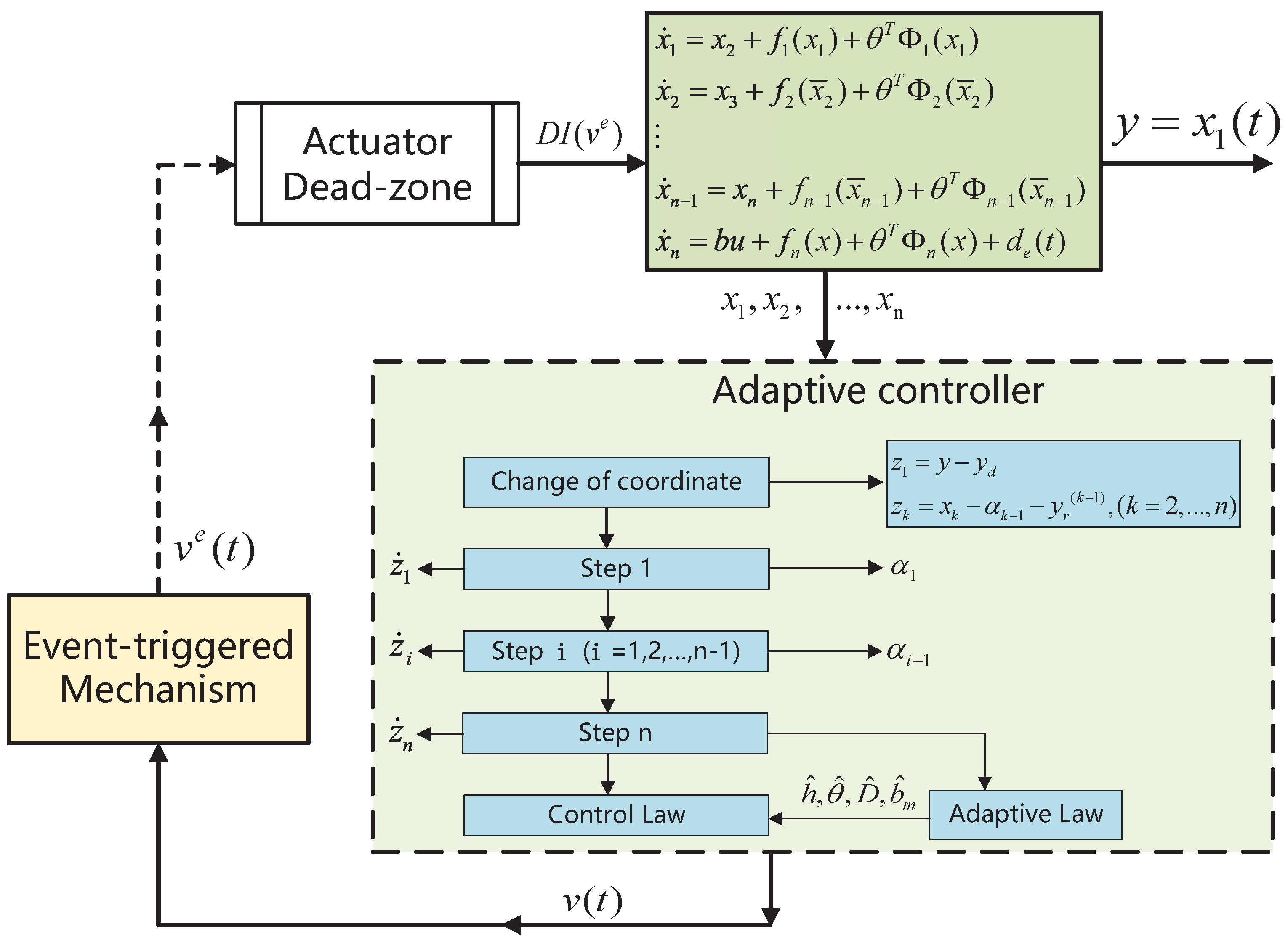
Consider a class of nonlinear systems described by the following state–space model:

$$\begin{array}{c}{\dot{x}}_1=x_2+f_1\left(x_1\right)+{\theta }^T{\Phi }_1\left(x_1\right)\hfill \\ {\dot{x}}_2=x_3+f_2\left({\overline{x}}_2\right)+{\theta }^T{\Phi }_2\left({\overline{x}}_2\right)\hfill \\ ⋮\hfill \\ {\dot{x}}_{n-1}=x_n+f_{n-1}\left({\overline{x}}_{n-1}\right)+{\theta }^T{\Phi }_{n-1}\left({\overline{x}}_{n-1}\right)\hfill \\ {\dot{x}}_n=bu+f_n\left(x\right)+{\theta }^T{\Phi }_n\left(x\right)+d_e\left(t\right)\hfill \\ y=x_1\hfill \end{array}$$

(1)

where ${\overline{x}}_i=(x_1,\dots ,x_i),x={(x_1,x_2,\dots ,x_n)}^T$ are system states, $u\in R$ is the input, and y is the output. Functions $f_i\left(x\right)\in R,{\varphi }_i\left(x\right)\in R^r$ $(i=1,2,\dots ,n)$ are known, and parameters $b\in R$ and $\theta \in R^r$ are unknown parameters. The unknown $d_e\left(t\right)$ is the external disturbance. All commonly used notations can be seen in

Table 1. Commonly used notations.

Symbol	Meaning	Symbol	Meaning
$x_i$	The state of the system	y	The input of the system
u	The input signal	$d_e\left(t\right)$	The external disturbance of the system
${\alpha }_i$	The virtual control	$d_{\delta }\left(t\right)$	The threshold interference
$DI\left(v\right)$	The dead-zone model	$y_r$	The reference signal
$sign(·)$	The sign function	$sg(·)$	The approximate function
V	Lyapunov function	$v^T,u^T$	Signals triggered

.

Consider the following dead-zone input:

$$u=DI\left(v\right)=\left\{\begin{array}{cc}m(v-b_r)& v\ge b_r\\ 0& b_l<v<b_r\\ m(v-b_l)& v\le b_l\end{array}\right.$$

(2)

where $m,b_r$ are unknown positive constants and parameter $b_l<0$ is a constant. In the dead-zone model $u=DI\left(v\right)$, u and v represent the output signal and input signal of the dead zone, respectively. Considering the dead-zone input, the system model can be written as

$$\begin{array}{ccc}\hfill {\dot{x}}_1& =& x_2+f_1\left(x_1\right)+{\theta }^T{\Phi }_1\left(x_1\right)\hfill \\ \hfill {\dot{x}}_i& =& x_{i+1}+f_i\left({\overline{x}}_i\right)+{\theta }^T{\Phi }_i\left({\overline{x}}_i\right)(i=2,\cdots ,n-1)\hfill \\ \hfill {\dot{x}}_n& =& bDI\left(v\right)+f_n\left(x\right)+{\theta }^T{\Phi }_n\left(x\right)+d_e\left(t\right)\hfill \\ \hfill y& =& x_1\hfill \end{array}$$

(3)

To proceed with the event-triggered adaptive backstepping controller, the following assumptions are made.

Assumption 1.

Unknown parameter $b\ne 0$ and $sign\left(b\right)$ is known. Without loss of generality, we take $b>0$ in this paper.

Assumption 2.

Reference signal $y_r\left(t\right)$ and its i-order $(i=1,\cdots ,n-1)$ derivatives are known and bounded.

To make the paper easier to understand, the following list of commonly used notations is provided.

3. Design and Analysis of Adaptive Controllers

3.1. Controller Design

Firstly, the following change in coordinates is introduced:

$$\begin{array}{ccc}\hfill z_1& =& x_1-y_r\hfill \\ \hfill z_i& =& x_i-{\alpha }_{i-1}-y_r^{(i-1)},(i=2,\dots ,n)\hfill \end{array}$$

(4)

where ${\alpha }_{i-1}$ $(i=1,2,\dots ,n)$ denote the virtual control in the $(i-1)th$ step.

Step 1: From (3) and the change in coordinates (4), the derivative of $z_1$ can be rewritten as

$${\dot{z}}_1=z_2+{\alpha }_1+f_1\left(x_1\right)+{\theta }^T{\Phi }_1\left(x_1\right)$$

(5)

where ${\alpha }_1$ is considered a virtual control. Consider the following Lyapunov function:

$$V_1=\frac{1}{2}{z}_1^2+\frac{1}{2}{\tilde{\theta }}^T{\Gamma }^{-1}\tilde{\theta }$$

(6)

where $\Gamma$ is a positive definite matrix. Because $\Gamma$ is a positive definite matrix, its inverse matrix ${\Gamma }^{-1}$ is also positive definite. Therefore, the term $\frac{1}{2}{\tilde{\theta }}^T{\Gamma }^{-1}\tilde{\theta }$ is a quadratic form and is non-negative. So, $V_1$ shown above satisfies the requirement as a Lyapunov function. The variable $\tilde{\theta }=\theta -\widehat{\theta }$ represents the estimation error, and $\widehat{\theta }$ is the estimation of $\theta$. Based on $V_1$ shown in (6), virtual control ${\alpha }_1$ can be chosen as

$${\alpha }_1=-k_1{z}_1-f_1\left(x_1\right)-{\widehat{\theta }}^T{\Phi }_1\left(x_1\right)$$

(7)

where $k_1>0$ is a design parameter. The derivative of $V_1$ is

$$\begin{array}{ccc}\hfill {\dot{V}}_1& =& z_1{\dot{z}}_1-{\tilde{\theta }}^T{\Gamma }^{-1}\dot{\widehat{\theta }}\hfill \\ & \le & z_1{z}_2-k_1{z}_1^2-{\tilde{\theta }}^T{\Gamma }^{-1}(\dot{\widehat{\theta }}-{\tau }_1)\hfill \end{array}$$

(8)

The tuning function ${\tau }_1$ is

$$\begin{array}{c}\hfill {\tau }_1=\Gamma {\Phi }_1{z}_1\end{array}$$

(9)

Next, we directly give the virtual control ${\alpha }_i$ and the Lyapunov function $V_i$ of step i.

Step $i(i=2,\dots ,n-1)$: The virtual control ${\alpha }_i$ can be chosen as

$$\begin{array}{ccc}\hfill {\alpha }_i& =& -k_i{z}_i-z_{i-1}+\sum _{j=1}^{i-1}(\frac{\partial {\alpha }_{i-1}}{\partial x_j}{x}_{j+1}+\frac{\partial {\alpha }_{i-1}}{\partial y_r^{(j-1)}}{y}_r^{\left(j\right)})-f_i\left({\overline{x}}_i\right)+\sum _{j=1}^{i-1}\frac{\partial {\alpha }_{i-1}}{\partial x_j}{f}_j\left({\overline{x}}_j\right)\hfill \\ & & +\frac{\partial {\alpha }_{i-1}}{\partial \widehat{\theta }}({\tau }_i-\Gamma l_{\theta }(\widehat{\theta }-{\theta }_0))-({\widehat{\theta }}^T-\sum _{k=2}^{i-1}{z}_k\frac{\partial {\alpha }_{k-1}}{\partial \widehat{\theta }}\Gamma \left)\right({\Phi }_i-\sum _{k=1}^{i-1}\frac{\partial {\alpha }_{i-1}}{\partial x_k}{\Phi }_k)\hfill \end{array}$$

(10)

where $k_i,l_{\theta },{\theta }_0$ are positive design parameters. The tuning function ${\tau }_i$ is

$$\begin{array}{c}\hfill {\tau }_i={\tau }_{i-1}+\Gamma \left({\Phi }_i-\sum _{k=1}^{i-1}\frac{\partial {\alpha }_{i-1}}{\partial x_k}{\Phi }_k\right)z_i\end{array}$$

(11)

and the Lyapunov function can be chosen as

$$V_i=V_{i-1}+\frac{1}{2}{z}_i^2$$

(12)

Step n: With (3), the derivative of $z_n$ is

$$\begin{array}{ccc}\hfill {\dot{z}}_n& =& bu+f_n\left(x\right)+{\theta }^T{\Phi }_n\left(x\right)-y_r^{\left(n\right)}-\sum _{j=1}^{n-1}\frac{\partial {\alpha }_{n-1}}{\partial y_r^{(j-1)}}{y}_r^{\left(j\right)}-\sum _{j=1}^{n-1}\frac{\partial {\alpha }_{n-1}}{\partial x_j}(x_{j+1}+f_j\left({\overline{x}}_j\right)+{\theta }^T{\Phi }_j\left({\overline{x}}_j\right))\hfill \\ & & -\frac{\partial {\alpha }_{n-1}}{\partial \widehat{\theta }}\dot{\widehat{\theta }}+d_e\left(t\right)\hfill \end{array}$$

(13)

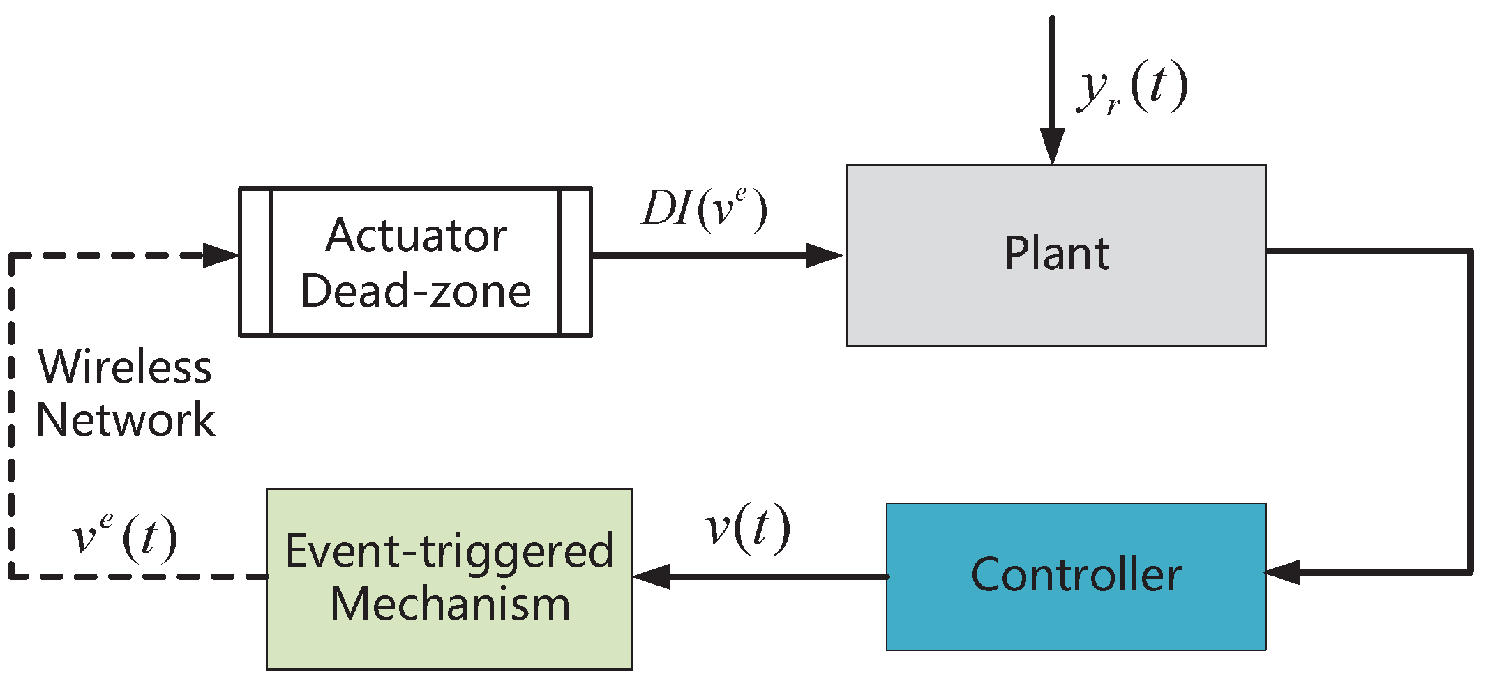
The event-triggered adaptive control scheme mainly includes an adaptive controller and a triggering mechanism. The block diagram is shown in Figure 1. Now, the input triggering mechanism can be designed as:

Triggering mechanism:

$$\begin{array}{ccc}\hfill & & v^T\left(t\right)=v\left(t_k\right),t\in [t_k,t_{k+1})\hfill \\ & & t_{k+1}=infimum\left\{t\in R:|v^e|\ge \sigma +d_{\sigma }\left(t\right)\right\}\hfill \\ & & t_1=0\hfill \end{array}$$

(14)

where $\sigma >0$ is a constant and $d_{\sigma }\left(t\right)$ represents the unknown disturbance. We suppose that the unknown disturbance $d_{\sigma }\left(t\right)$ satisfies

$$|d_{\sigma }\left(t\right)|\le D_{\sigma }$$

(15)

where $D_{\sigma }\ll \sigma$ is an unknown constant. $\left\{t_k\right\},k=0,1,\cdots$ are the event-triggering instants. The variable $v^T\left(t\right),t\in [t_1,t_2)$ is a constant, and its value is $v\left(t_1\right)$. The value of $v^T\left(t\right)$ is updated to $v\left(t_2\right)$ when $t_2$ is the first time instant to satisfy the condition $|v^e|\ge \sigma +d_{\sigma }\left(t\right)$. $v^e=v-v^T$ is the error between the input signal v and its triggered value.

Remark 1.

The above threshold for the triggering event on system input is reasonable in practice. As previously mentioned, external interference and small measurement errors are difficult to avoid in state sampling and in the calculation of the input signal value. This inevitably leads to errors between the true value of $v^e$ and the measured value. Such errors can be seen as external disturbances and need to be considered in the threshold construction. In a sense, then, the designed threshold is actually a variable threshold. This changing threshold makes controller design challenging, especially when the laws of change cannot be known.

Unlike standard backstepping, the control law and update laws of unknown parameters can be given as follows:

Control Law:

$$\begin{array}{ccc}\hfill v& =& \widehat{h}\alpha ;\alpha ={\alpha }_{n1}+{\alpha }_{n2}\hfill \\ \hfill {\alpha }_{n1}& =& -z_{n-1}-k_n{z}_n-\sum _{i=0}^4\frac{1}{4{\epsilon }_i}{z}_n-f_n\left(x\right)+y_r^{\left(n\right)}+\sum _{j=1}^{n-1}(\frac{\partial {\alpha }_{n-1}}{\partial x_j}(x_{j+1}+f_j\left({\overline{x}}_j\right))+\frac{\partial {\alpha }_{n-1}}{\partial y_r^{(j-1)}}{y}_r^{\left(j\right)})\hfill \\ & & +\frac{\partial {\alpha }_{n-1}}{\partial \widehat{\theta }}({\tau }_n-\Gamma l_{\theta }(\widehat{\theta }-{\theta }_0))-({\widehat{\theta }}^T-\sum _{k=2}^{n-1}{z}_k\frac{\partial {\alpha }_{k-1}}{\partial \widehat{\theta }}\Gamma \left)\right({\Phi }_n-\sum _{k=1}^{n-1}\frac{\partial {\alpha }_{n-1}}{\partial x_k}{\Phi }_k)\hfill \\ \hfill {\alpha }_{n2}& =& -{\widehat{b}}_{m}sg\left(z_n\right)\sigma -\widehat{D}sg\left(z_n\right)\hfill \end{array}$$

(16)

$$\begin{array}{ccc}\hfill {\tau }_n& =& {\tau }_{n-1}+\Gamma ({\Phi }_n-\sum _{k=1}^{n-1}\frac{\partial {\alpha }_{n-1}}{\partial x_k}{\Phi }_k)z_n\hfill \end{array}$$

(17)

$$sg\left(z_n\right)=\left\{\begin{array}{cc}\frac{z_n}{|z_n|},\hfill & |z_n|\ge \delta \hfill \\ \frac{z_n}{{\left({\delta }^2-z_n^2\right)}^2+|z_n|},\hfill & |z_n|<\delta \hfill \end{array}\right.$$

where $k_n$, ${\epsilon }_i$ are positive design parameters and $\delta$ is a positive constant. The variables $\widehat{h}$, ${\widehat{b}}_m$, and $\widehat{D}$ are the estimates of parameters $h=\frac{1}{b_m}$, $b_m=bm$, and $D=D_{DI}+D_{\sigma }+D_e$, respectively. The constants $D_{DI}$ and $D_e$ will be explained in detail in the following stability analysis section.

Remark 2.

The function $sg\left(z_n\right)$ can be seen as an approximation of $sign\left(z_n\right)$. Because $sign\left(z_n\right)$ is discontinuous, input signal v is also discontinuous when $sign\left(z_n\right)$ is used directly. If $sg\left(z_n\right)$ is used instead of a symbolic function, continuous control inputs can be obtained.

Update Laws:

$$\begin{array}{ccc}\hfill \dot{\widehat{h}}& =& -{\eta }_h\alpha z_n-{\eta }_h{l}_h(\widehat{h}-h_0)\hfill \\ \hfill \dot{\widehat{\theta }}& =& {\tau }_n-\Gamma l_{\theta }(\widehat{\theta }-{\theta }_0)\hfill \\ \hfill \dot{\widehat{D}}& =& {\eta }_D|z_n|-{\eta }_D{l}_D(\widehat{D}-D_0)\hfill \\ \hfill {\dot{\widehat{b}}}_m& =& {\eta }_b|z_n|\sigma -{\eta }_b{l}_b({\widehat{b}}_m-b_{m0})\hfill \end{array}$$

(18)

where ${\eta }_h,{\eta }_D,{\eta }_b,l_h,l_{\theta },l_D,l_b,h_0,{\theta }_0,D_0,b_{m0}$ are positive constants and $\Gamma$ is a positive definite matrix. The design parameters $h_0,{\theta }_0,D_0,b_{m0}$ are pre-estimated values of parameters $h,\theta ,D,b_m$, respectively. The closer these pre-estimated values are to the true values of these parameters, the better the tracking performance of the system will be.

Based on Figure 1 and the process of the controller design using backstepping, a block diagram of the closed-loop feedback system is shown in Figure 2.

3.2. Stability Analysis

Next, we will continue to analyze the derivative of $z_n$. Because under the event-triggering mechanism, the actual input signal acting on the system is $v^T$, from (13) we can obtain

$$\begin{array}{ccc}\hfill {\dot{z}}_n& =& bDI\left(v^T\right)+f_n\left(x\right)+{\theta }^T{\Phi }_n\left(x\right)-y_r^{\left(n\right)}-\sum _{j=1}^{n-1}\frac{\partial {\alpha }_{n-1}}{\partial x_j}(x_{j+1}+f_j\left({\overline{x}}_j\right)+{\theta }^T{\Phi }_j\left({\overline{x}}_j\right))\hfill \\ & & -\sum _{j=1}^{n-1}\frac{\partial {\alpha }_{n-1}}{\partial y_r^{(j-1)}}{y}_r^{\left(j\right)}-\frac{\partial {\alpha }_{n-1}}{\partial \widehat{\theta }}\dot{\widehat{\theta }}+d_e\left(t\right)\hfill \end{array}$$

(19)

Using

$$u^T=DI\left(v^T\right)=DI(v-v^e)$$

$$=\left\{\begin{array}{cc}m(v-b_r)-m{v}^e& v\ge b_r+v^e\\ 0& b_l+v^e<v<b_r+v^e\\ m(v-b_l)-m{v}^e& v\le b_l+v^e\end{array}\right.$$

(20)

and (2), we can obtain the following analysis results on $u^e=u-u^T$.

Lemma 1.

Signals u and $u^T$ are output signals of the nonlinear dead zone shown in (2). They are generated by v and $v^T$, respectively. The error $u^e$ between u and $u^T$ is bounded by an unknown constant such that

$$\begin{array}{c}\hfill |u^e|\le m|v^e|+m(b_r-b_l)\end{array}$$

(21)

Proof. 

In the following, we discuss two cases:

• $v^e>0$
  (1) $b_l+v^e<b_r$

  $$u^e=\left\{\begin{array}{cc}m{v}^e& v\ge b_r+v^e\\ m(v-b_r)& b_r<v<b_r+v^e\\ 0& b_l+v^e<v\le b_r\\ m{v}^e-m(v-b_l)& b_l<v\le b_r+v^e\\ m{v}^e& v\le b_l\end{array}\right.$$

  (22)
  Because

  $$|m(v-b_r)|\le m|v^e|,\forall b_r<v<b_r+v^e,$$

  and note that $0<v^e<b_r-b_l$, we have

  $$|m{v}^e-m(v-b_l)|\le m(b_r-b_l),\forall b_l<v\le b_r+v^e$$
  Then, we have

  $$|u^e|\le m(b_r-b_l)$$

  (23)
  (2) $b_l+v^e\ge b_r$

  $$u^e=\left\{\begin{array}{cc}m{v}^e& v\ge b_r+v^e\\ m(v-b_r)& b_l+v^e\le v<b_r+v^e\\ m(b_l-b_r)+m{v}^e& b_r\le v<b_l+v^e\\ m{v}^e-m(v-b_l)& b_l\le v<b_r\\ m{v}^e& v\le b_l\end{array}\right.$$

  (24)
  Because

  $$|m(v-b_r)|\le m|v^e|,\forall b_l+v^e<v<b_r+v^e,$$

  and note that $0<b_r-b_l<v^e$, we have

  $$|m{v}^e-m(v-b_l)|\le m|v^e|,\forall b_l<v\le b_r$$
  Then, we have

  $$|u^e|\le m|v^e|$$

  (25)
• $v^e\le 0$
  (1) $b_l<b_r+v^e$

  $$u^e=\left\{\begin{array}{cc}m{v}^e& v\ge b_r\\ m{v}^e-m(v-b_r)& b_r+v^e\le v<b_r\\ 0& b_l\le v<b_r+v^e\\ m(v-b_l)& b_l+v^e\le v<b_l\\ m{v}^e& v\le b_l+v^e\end{array}\right.$$

  (26)
  Because

  $$|m(v-b_l)|\le m|v^e|,\forall b_l+v^e\le v<b_l$$

  and

  $$|m{v}^e-m(v-b_r)|\le m|v^e|,\forall b_r+v^e\le v<b_r$$

  we have

  $$|u^e|\le m|v^e|$$

  (27)
  (2) $b_r+v^e\le b_l$

  $$u^e=\left\{\begin{array}{cc}m{v}^e& v\ge b_r\\ m{v}^e-m(v-b_r)& b_l\le v<b_r\\ m{v}^e+m(b_r-b_l)& b_r+v^e\le v<b_l\\ m(v-b_l)& b_l+v^e\le v<b_r+v^e\\ m{v}^e& v\le b_l+v^e\end{array}\right.$$

  (28)
  Because

  $$|m(v-b_l)|\le m|v^e|+m(b_r-b_l),\forall b_l+v^e\le v<b_r+v^e$$

  and

  $$|m{v}^e+m(b_r-b_l)|\le m|v^e|+m(b_r-b_l),\forall b_r+v^e\le v<b_l$$

  and

  $$|m{v}^e-m(v-b_r)|\le m|v^e|+m(b_r-b_l),\forall b_l\le v<b_r$$

  we have

  $$|u^e|\le m|v^e|+m(b_r-b_l)$$

  (29)

With (23), (25), (27), and (29), we obtain

$$|u^e|\le m|v^e|+m(b_r-b_l)$$

(30)

 □

From (19), we have

$$\begin{array}{ccc}\hfill {\dot{z}}_n& =& b[DI\left(v^T\right)-DI\left(v\right)]+bDI\left(v\right)+f_n\left(x\right)+{\theta }^T{\Phi }_n\left(x\right)-\sum _{j=1}^{n-1}\frac{\partial {\alpha }_{n-1}}{\partial x_j}(x_{j+1}+f_j({\overline{x}}_j)+{\theta }^T{\Phi }_j({\overline{x}}_j))\hfill \\ & & -y_r^{\left(n\right)}-\sum _{j=1}^{n-1}\frac{\partial {\alpha }_{n-1}}{\partial y_r^{(j-1)}}{y}_r^{\left(j\right)}-\frac{\partial {\alpha }_{n-1}}{\partial \widehat{\theta }}\dot{\widehat{\theta }}+d_e\left(t\right)\hfill \end{array}$$

(31)

Note that the symmetrical dead zone considered here can be linearized by using the linear approximation $DI\left(v\right)=mv+{\overline{d}}_{DI}$. The unknown ${\overline{d}}_{DI}$ is the approximation error and bounded by an unknown constant:

$$\begin{array}{ccc}\hfill {\dot{z}}_n& =& -b{u}^e+b_{m}v+d_{DI}+f_n\left(x\right)+{\theta }^T{\Phi }_n\left(x\right)-y_r^{\left(n\right)}-\sum _{j=1}^{n-1}\frac{\partial {\alpha }_{n-1}}{\partial x_j}(x_{j+1}+f_j({\overline{x}}_j)+{\theta }^T{\Phi }_j({\overline{x}}_j))\hfill \\ & & -\sum _{j=1}^{n-1}\frac{\partial {\alpha }_{n-1}}{\partial y_r^{(j-1)}}{y}_r^{\left(j\right)}-\frac{\partial {\alpha }_{n-1}}{\partial \widehat{\theta }}\dot{\widehat{\theta }}+d_e\left(t\right)\hfill \end{array}$$

(32)

where $b_m=bm>0$ is an unknown constant and $d_{DI}=b{\overline{d}}_{DI}$ is a function of the time variable t. Because b is a constant and ${\overline{d}}_{DI}$ is bounded, $d_{DI}$ is bounded by an unknown constant $D_{DI}$.

Next, we can establish our main result as stated in the following theorem.

Theorem 1.

Consider a closed-loop system consisting of system (1), dead-zone input (2), controller (14), (16), and update laws (18). Under Assumptions 1 and 2, the following results hold:

• All signals in the closed-loop system are globally bounded, and the Zeno behavior can be avoided.
• The tracking error satisfies

  $$li{m}_{t\to \infty }|y\left(t\right)-y_r|\le \sqrt{\frac{2{\hslash }_1}{{\hslash }_2}\Xi }$$

  (33)

  where ${\hslash }_1$ and ${\hslash }_1$ are constants and Ξ is bounded by a constant.

Proof. 

Note that

$$\widehat{h}{b}_{m}v=b_m(h-\tilde{h})v=v-b_m\tilde{h}v$$

(34)

where $\tilde{h}=h-\widehat{h}$. With (34), Equation (32) can be written as

$$\begin{array}{ccc}\hfill {\dot{z}}_n& =& -b{u}^e-b_m\tilde{h}\alpha +\alpha +d_{DI}+f_n\left(x\right)+{\theta }^T{\Phi }_n\left(x\right)-y_r^{\left(n\right)}-\sum _{j=1}^{n-1}\frac{\partial {\alpha }_{n-1}}{\partial x_j}\left(x_{j+1}+f_j\left({\overline{x}}_j\right)+{\theta }^T{\Phi }_j\left({\overline{x}}_j\right)\right)\hfill \\ & & -\sum _{j=1}^{n-1}\frac{\partial {\alpha }_{n-1}}{\partial y_r^{(j-1)}}{y}_r^{\left(j\right)}-\frac{\partial {\alpha }_{n-1}}{\partial \widehat{\theta }}\dot{\widehat{\theta }}+d_e\left(t\right)\hfill \end{array}$$

(35)

Then, with (16), we have

$$\begin{array}{ccc}\hfill {(\frac{z_n^2}{2})}^{\prime }& =& z_n{\dot{z}}_n\hfill \\ & =& z_n(-b{u}^e-b_m\tilde{h}\alpha +d_{DI}+d_e\left(t\right)+{\theta }^T{\Phi }_n\left(x\right)-\sum _{j=1}^{n-1}\frac{\partial {\alpha }_{n-1}}{\partial x_j}{\theta }^T{\Phi }_j\left({\overline{x}}_j\right)-\frac{\partial {\alpha }_{n-1}}{\partial \widehat{\theta }}\dot{\widehat{\theta }}-z_{n-1}\hfill \\ & & -k_n{z}_n+\frac{\partial {\alpha }_{n-1}}{\partial \widehat{\theta }}{\tau }_n-\frac{\partial {\alpha }_{n-1}}{\partial \widehat{\theta }}\Gamma l_{\theta }(\widehat{\theta }-{\theta }_0)-\left({\widehat{\theta }}^T-\sum _{k=2}^{n-1}{z}_k\frac{\partial {\alpha }_{k-1}}{\partial \widehat{\theta }}\Gamma \right)\left({\Phi }_n-\sum _{k=1}^{n-1}\frac{\partial {\alpha }_{n-1}}{\partial x_k}{\Phi }_k\right)\hfill \\ & & -{\widehat{b}}_{m}sg\left(z_n\right)\sigma -\widehat{D}sg\left(z_n\right)-\sum _{i=0}^4\frac{1}{4{\epsilon }_i}{z}_n)\hfill \end{array}$$

(36)

$$\begin{array}{ccc}& =& z_n(-b{u}^e-b_m\tilde{h}\alpha +d_{DI}+d_e\left(t\right)+{\theta }^T{\Phi }_n\left(x\right)-\sum _{j=1}^{n-1}\frac{\partial {\alpha }_{n-1}}{\partial x_j}{\theta }^T{\Phi }_j\left({\overline{x}}_j\right)-\frac{\partial {\alpha }_{n-1}}{\partial \widehat{\theta }}\dot{\widehat{\theta }}-z_{n-1}\hfill \\ & & -k_n{z}_n+\frac{\partial {\alpha }_{n-1}}{\partial \widehat{\theta }}{\tau }_n-\frac{\partial {\alpha }_{n-1}}{\partial \widehat{\theta }}\Gamma l_{\theta }(\widehat{\theta }-{\theta }_0)-\left({\widehat{\theta }}^T-\sum _{k=2}^{n-1}{z}_k\frac{\partial {\alpha }_{k-1}}{\partial \widehat{\theta }}\Gamma \right)\left({\Phi }_n-\sum _{k=1}^{n-1}\frac{\partial {\alpha }_{n-1}}{\partial x_k}{\Phi }_k\right)\hfill \\ & & -{\widehat{b}}_{m}sign\left(z_n\right)\sigma -\widehat{D}sign\left(z_n\right)-\sum _{i=0}^4\frac{1}{4{\epsilon }_i}{z}_n+({\widehat{b}}_m\sigma +\widehat{D})(sign\left(z_n\right)-sg\left(z_n\right)))\hfill \end{array}$$

Now consider the following Lyapunov function

$$\begin{array}{c}\hfill V_n=V_{n-1}+\frac{1}{2}{z}_n^2+\frac{b_m}{2{\eta }_h}{\tilde{h}}^2+\frac{1}{2{\eta }_D}{\tilde{D}}^2+\frac{1}{2{\eta }_b}{\tilde{b}}_m^2\end{array}$$

(37)

where $\tilde{h}=h-\widehat{h}$, $\tilde{D}=D-\widehat{D}$ and ${\tilde{b}}_m=b_m-{\widehat{b}}_m$ represent estimation errors of $h,D$, and $b_m$, respectively. With (36), the derivative of $V_n$ is

$$\begin{array}{ccc}\hfill {\dot{V}}_n& \le & -\sum _{j=1}^n{k}_j{z}_j^2-\sum _{i=0}^4\frac{1}{4{\epsilon }_i}{z}_n^2-{\tilde{\theta }}^T{\Gamma }^{-1}(\dot{\widehat{\theta }}-{\tau }_n)-\left(\sum _{j=1}^{n-1}{z}_{j+1}\frac{\partial {\alpha }_j}{\partial \widehat{\theta }}\right)(\dot{\widehat{\theta }}-{\tau }_n+\Gamma l_{\theta }(\widehat{\theta }-{\theta }_0))\hfill \\ & & -\frac{b_m}{{\eta }_h}\tilde{h}(\dot{\widehat{h}}+{\eta }_h\alpha z_n)-b{z}_n{u}^e+z_n{d}_{DI}+z_n{d}_e\left(t\right)-|z_n|{\widehat{b}}_m\sigma -|z_n|\widehat{D}-\frac{\tilde{D}}{{\eta }_D}\dot{\widehat{D}}-\frac{{\tilde{b}}_m}{{\eta }_b}{\dot{\widehat{b}}}_m\hfill \\ & & +({\widehat{b}}_m\sigma +\widehat{D})(sign\left(z_n\right)-sg\left(z_n\right))z_n\hfill \end{array}$$

(38)

Note that

$$\begin{array}{ccc}\hfill -b{z}_n{u}^e& \le & b|z_n|u^e\hfill \\ & =& |z_n|b_m\sigma +|z_n|b_m(b_r-b_l)+|z_n|b_m|d_{\sigma }|\hfill \\ & \le & |z_n|b_m\sigma +|z_n|b_m(b_r-b_l)+|z_n|b_m{D}_{\sigma }\hfill \end{array}$$

(39)

and

$$\begin{array}{c}\hfill z_n{d}_{DI}\le |z_n|D_{DI};z_n{d}_e\left(t\right)\le |z_n|D_e\end{array}$$

(40)

we have

$$\begin{array}{ccc}\hfill {\dot{V}}_n& \le & -\sum _{j=1}^n{k}_j{z}_j^2-{\tilde{\theta }}^T{\Gamma }^{-1}(\dot{\widehat{\theta }}-{\tau }_n)-\frac{b_m}{{\eta }_h}\tilde{h}(\dot{\widehat{h}}+{\eta }_h\alpha z_n)-\left(\sum _{j=1}^{n-1}{z}_{j+1}\frac{\partial {\alpha }_j}{\partial \widehat{\theta }}\right)(\dot{\widehat{\theta }}-{\tau }_n+\Gamma l_{\theta }(\widehat{\theta }-{\theta }_0))\hfill \\ & & -|z_n|{\widehat{b}}_m\sigma +z_n(D_{DI}+D_e+D_{\sigma })-|z_n|\widehat{D}+|z_n|b_m(b_r-b_l)-\sum _{i=0}^4\frac{1}{4{\epsilon }_i}{z}_n^2-\frac{\tilde{D}}{{\eta }_D}\dot{\widehat{D}}-\frac{{\tilde{b}}_m}{{\eta }_b}{\dot{\widehat{b}}}_m\hfill \\ & & +|z_n|b_m\sigma +({\widehat{b}}_m\sigma +\widehat{D})(sign\left(z_n\right)-sg\left(z_n\right))z_n\hfill \end{array}$$

(41)

Letting

$$\begin{array}{c}\hfill D=D_{DI}+D_e+D_{\sigma }\end{array}$$

(42)

we obtain

$$\begin{array}{ccc}\hfill {\dot{V}}_n& \le & -\sum _{j=1}^n{k}_j{z}_j^2-{\tilde{\theta }}^T{\Gamma }^{-1}(\dot{\widehat{\theta }}-{\tau }_n)-\frac{b_m}{{\eta }_h}\tilde{h}(\dot{\widehat{h}}+{\eta }_h\alpha z_n)-\left(\sum _{j=1}^{n-1}{z}_{j+1}\frac{\partial {\alpha }_j}{\partial \widehat{\theta }}\right)(\dot{\widehat{\theta }}-{\tau }_n+\Gamma l_{\theta }(\widehat{\theta }-{\theta }_0))\hfill \\ & & +|z_n|b_m\sigma -|z_n|{\widehat{b}}_m\sigma +z_{n}D-|z_n|\widehat{D}+|z_n|b_m(b_r-b_l)-\sum _{i=0}^4\frac{1}{4{\epsilon }_i}{z}_n^2-\frac{\tilde{D}}{{\eta }_D}\dot{\widehat{D}}-\frac{{\tilde{b}}_m}{{\eta }_b}{\dot{\widehat{b}}}_m\hfill \\ & & +({\widehat{b}}_m\sigma +\widehat{D})(sign\left(z_n\right)-sg\left(z_n\right))z_n\hfill \end{array}$$

(43)

Note that

$$\begin{array}{c}\hfill |z_n|b_m\sigma -|z_n|{\widehat{b}}_m\sigma -\frac{{\tilde{b}}_m}{{\eta }_b}{\dot{\widehat{b}}}_m=-\frac{{\tilde{b}}_m}{{\eta }_b}({\dot{\widehat{b}}}_m-{\eta }_b|z_n|\sigma )\end{array}$$

(44)

$$\begin{array}{c}\hfill z_{n}D-|z_n|\widehat{D}-\frac{\tilde{D}}{{\eta }_D}\dot{\widehat{D}}=-\frac{\tilde{D}}{{\eta }_D}(\dot{\widehat{D}}-{\eta }_D|z_n|)\end{array}$$

(45)

$$\begin{array}{ccc}\hfill |z_n|b_m(b_r-b_l)-\frac{1}{4{\epsilon }_0}{z}_n^2& \le & \frac{1}{4{\epsilon }_0}{z}_n^2+{\epsilon }_0{\left(b_m(b_r-b_l)\right)}^2-\frac{1}{4{\epsilon }_0}{z}_n^2\hfill \\ & =& {\epsilon }_0{\left(b_m(b_r-b_l)\right)}^2\hfill \end{array}$$

(46)

we have

$$\begin{array}{ccc}\hfill {\dot{V}}_n& \le & -\sum _{j=1}^n{k}_j{z}_j^2-{\tilde{\theta }}^T{\Gamma }^{-1}(\dot{\widehat{\theta }}-{\tau }_n)-\frac{b_m}{{\eta }_h}\tilde{h}(\dot{\widehat{h}}+{\eta }_h\alpha z_n)-\left(\sum _{j=1}^{n-1}{z}_{j+1}\frac{\partial {\alpha }_j}{\partial \widehat{\theta }}\right)(\dot{\widehat{\theta }}-{\tau }_n+\Gamma l_{\theta }(\widehat{\theta }-{\theta }_0))\hfill \\ & & -\frac{{\tilde{b}}_m}{{\eta }_b}({\dot{\widehat{b}}}_m-{\eta }_b|z_n|\sigma )-\frac{\tilde{D}}{{\eta }_D}(\dot{\widehat{D}}-{\eta }_D|z_n|)+{\epsilon }_0{\left(b_m(b_r-b_l)\right)}^2-\sum _{i=1}^4\frac{1}{4{\epsilon }_i}{z}_n^2\hfill \\ & & +({\widehat{b}}_m\sigma +\widehat{D})(sign\left(z_n\right)-sg\left(z_n\right))z_n\hfill \end{array}$$

(47)

With update laws (18) and

$$\begin{array}{c}\hfill l_h\tilde{h}(\widehat{h}-h_0)\le -\frac{1}{2}{l}_h{\tilde{h}}^2+\frac{1}{2}{l}_h{(h-h_0)}^2\end{array}$$

(48)

$$\begin{array}{c}\hfill l_D\tilde{D}(\widehat{D}-D_0)\le -\frac{1}{2}{l}_D{\tilde{D}}^2+\frac{1}{2}{l}_D{(D-D_0)}^2\end{array}$$

(49)

$$\begin{array}{c}\hfill l_b{\tilde{b}}_m({\widehat{b}}_m-b_{m0})\le -\frac{1}{2}{l}_b{\tilde{b}}_m^2+\frac{1}{2}{l}_b{(b_m-b_{m0})}^2\end{array}$$

(50)

$$\begin{array}{c}\hfill l_{\theta }{\tilde{\theta }}^T(\widehat{\theta }-{\theta }_0)\le -\frac{1}{2}{l}_{\theta }||\tilde{\theta }{||}_2^2+\frac{1}{2}{l}_{\theta }||\theta -{\theta }_0{||}^2\end{array}$$

(51)

we have

$$\begin{array}{ccc}\hfill {\dot{V}}_n& \le & -\sum _{j=1}^n{k}_j{z}_j^2-\frac{1}{2}{l}_{\theta }||\tilde{\theta }{||}_2^2-\frac{1}{2}{l}_h{\tilde{h}}^2-\frac{1}{2}{l}_D{\tilde{D}}^2-\frac{1}{2}{l}_b{\tilde{b}}_m^2+{\Xi }_1-\sum _{i=1}^4\frac{1}{4{\epsilon }_i}{z}_n^2\hfill \\ & & +({\widehat{b}}_m\sigma +\widehat{D})(sign\left(z_n\right)-sg\left(z_n\right))z_n\hfill \end{array}$$

(52)

where

$$\begin{array}{ccc}\hfill {\Xi }_1& =& \frac{1}{2}{l}_h{(h-h_0)}^2+\frac{1}{2}{l}_D{(D-D_0)}^2+\frac{1}{2}{l}_b{(b_m-b_{m0})}^2\hfill \\ & & +\frac{1}{2}{l}_{\theta }||\theta -{\theta }_0{||}^2+{\epsilon }_0{\left(b_m(b_r-b_l)\right)}^2\hfill \end{array}$$

(53)

Note that

$$\begin{array}{c}\hfill \widehat{D}(sign\left(z_n\right)-sg\left(z_n\right))z_n=(D-\tilde{D})(sign\left(z_n\right)-sg\left(z_n\right))z_n\end{array}$$

(54)

and

$$\begin{array}{ccc}\hfill D(sign\left(z_n\right)-sg\left(z_n\right))z_n& \le & \frac{1}{4{\epsilon }_1}{z}_n^2+{\epsilon }_1{\left((sign\left(z_n\right)-sg\left(z_n\right))D\right)}^2-\tilde{D}(sign\left(z_n\right)-sg\left(z_n\right))z_n\hfill \\ & \le & \frac{1}{4{\epsilon }_2}{z}_n^2+{\epsilon }_2{\left((sign\left(z_n\right)-sg\left(z_n\right))\tilde{D}\right)}^2\hfill \end{array}$$

(55)

Similar to (54) and (55), we have

$$\begin{array}{c}\hfill {\widehat{b}}_m\sigma (sign\left(z_n\right)-sg\left(z_n\right))z_n=(b_m-{\tilde{b}}_m)\sigma (sign\left(z_n\right)-sg\left(z_n\right))z_n\end{array}$$

(56)

and

$$\begin{array}{ccc}\hfill b_m\sigma (sign\left(z_n\right)-sg\left(z_n\right))z_n& \le & \frac{1}{4{\epsilon }_3}{z}_n^2+{\epsilon }_3{\left(\sigma (sign\left(z_n\right)-sg\left(z_n\right))b_m\right)}^2-{\tilde{b}}_m\sigma (sign\left(z_n\right)-sg\left(z_n\right))z_n\hfill \\ & \le & \frac{1}{4{\epsilon }_4}{z}_n^2+{\epsilon }_4{\left(\sigma (sign\left(z_n\right)-sg\left(z_n\right)){\tilde{b}}_m\right)}^2\hfill \end{array}$$

(57)

we have

$$\begin{array}{ccc}\hfill {\dot{V}}_n& \le & -\sum _{j=1}^n{k}_j{z}_j^2-\frac{1}{2}{l}_{\theta }||\tilde{\theta }{||}_2^2-\frac{1}{2}{l}_h{\tilde{h}}^2-\frac{1}{2}{l}_D{\tilde{D}}^2-\frac{1}{2}{l}_b{\tilde{b}}_m^2+{\epsilon }_2{\left((sign\left(z_n\right)-sg\left(z_n\right))\tilde{D}\right)}^2\hfill \\ & & +{\epsilon }_4{\left(\sigma (sign\left(z_n\right)-sg\left(z_n\right)){\tilde{b}}_m\right)}^2+\Xi \hfill \end{array}$$

(58)

where

$$\begin{array}{c}\hfill \Xi ={\Xi }_1+{\epsilon }_1{\left((sign\left(z_n\right)-sg\left(z_n\right))D\right)}^2+{\epsilon }_3{\left(\sigma (sign\left(z_n\right)-sg\left(z_n\right))b_m\right)}^2\end{array}$$

(59)

Then, we obtain

$$\begin{array}{ccc}\hfill {\dot{V}}_n& \le & -\sum _{j=1}^n{k}_j{z}_j^2-\frac{1}{2}{l}_{\theta }||\tilde{\theta }{||}_2^2-\frac{1}{2}{l}_h{\tilde{h}}^2-\frac{1}{2}{\overline{l}}_D{\tilde{D}}^2-\frac{1}{2}{\overline{l}}_b{\tilde{b}}_m^2+\Xi \hfill \end{array}$$

(60)

where

$$\begin{array}{c}{\overline{l}}_D=l_D-{\epsilon }_2{(sign\left(z_n\right)-sg\left(z_n\right))}^2\hfill \\ {\overline{l}}_b=l_b-{\epsilon }_4{\left(\sigma (sign\left(z_n\right)-sg\left(z_n\right))\right)}^2\hfill \end{array}$$

(61)

Let

$$V=\sum _{i=1}^n{z}_i^2+||\tilde{\theta }{||}_2^2+{\tilde{h}}^2+{\tilde{D}}^2+{\tilde{b}}_m^2$$

(62)

Obviously, we have

$$V_n\le {\hslash }_{1}V$$

(63)

where

$${\hslash }_1=max\left\{\frac{1}{2},\frac{1}{2}{\lambda }_{max}\left({\Gamma }^{-1}\right),\frac{b_m}{2{\eta }_h},\frac{1}{2{\eta }_D},\frac{1}{2{\eta }_b}\right\}$$

(64)

The constant ${\lambda }_{max}\left({\Gamma }^{-1}\right)$ is the maximum eigenvalue of matrix ${\Gamma }^{-1}$.

From (60), we obtain

$$\begin{array}{ccc}\hfill {\dot{V}}_n& \le & -{\hslash }_{2}V+\Xi \hfill \end{array}$$

(65)

where

$$\begin{array}{c}\hfill {\hslash }_2=min\{k_j(j=1,\cdots ,n),\frac{1}{2}{l}_{\theta },\frac{1}{2}{l}_h,\frac{1}{2}{\overline{l}}_D,\frac{1}{2}{\overline{l}}_b\}\end{array}$$

(66)

Then, we have

$${\dot{V}}_n\le -{\hslash }_{2}V+\Xi \le -\frac{{\hslash }_2}{{\hslash }_1}{V}_n+\Xi$$

(67)

By the direct integration of the differential inequality, we have

$$V_n\le V_n\left(0\right)e^{-\frac{{\hslash }_2}{{\hslash }_1}t}+\frac{{\hslash }_1}{{\hslash }_2}\Sigma$$

(68)

Note that $e^{-\frac{{\hslash }_2}{{\hslash }_1}t}$ is a monotonic decreasing function because of $\frac{{\hslash }_2}{{\hslash }_1}>0$, and $\Xi$ is bounded. Then, we can obtain that $V_n$ is bounded. Thus, $z_i,\tilde{\theta },\tilde{h},\tilde{D},{\tilde{b}}_m$ are bounded. Furthermore, $x_i$ and v are also bounded. Hence, we can obtain that all the signals of the closed-loop system are bounded. Hence, all the signals of closed-loop system are ensured to be bounded.

Because v is differentiable, the derivative function $\dot{v}$ is continuous. Due to all signals in the closed-loop system being bounded, $\dot{v}$ is bounded. Namely, there exists a constant $\pi$ such that $|\dot{v}|\le \pi$. We therefore easily have

$$\begin{array}{c}\hfill \frac{d}{dt}|v^e|=\frac{d}{dt}{(v^e\ast v^e)}^{\frac{1}{2}}=sign\left(v^e\right){\dot{v}}^e\le |\dot{v}|\end{array}$$

(69)

According to the Lagrange mean value theorem, we have

$$v^e\left(t_{k+1}\right)-v^e\left(t_k\right)={\dot{v}}^e\left(\xi \right)(t_{k+1}-t_k)$$

By noting that $v^e\left(t_k\right)=0$ and $li{m}_{t\to t_{k+1}}{v}^e\left(t\right)=\sigma +d_{\sigma }\left(t_{k+1}\right)$, we have

$$\begin{array}{c}\hfill t_{k+1}-t_k\ge \frac{\sigma +d_{\sigma }\left(t_{k+1}\right)}{\pi }\ge \frac{\sigma -D_{\sigma }}{\pi }\end{array}$$

(70)

Thus, the Zeno behavior can be avoided.

If $|y\left(t\right)-y_r|>\sqrt{\frac{2{\hslash }_1}{{\hslash }_2}\Xi }$, then from (67)

$${\dot{V}}_n\le -{\hslash }_{2}V+\Xi \le -\frac{{\hslash }_2}{{\hslash }_1}{V}_n+\Xi <0$$

(71)

So, $V_n$ will decrease until $|y\left(t\right)-y_r|\le \sqrt{\frac{2{\hslash }_1}{{\hslash }_2}\Xi }$.  □

Remark 3.

From the definition of function $sg(·)$ shown in (16), we can obtain $sign\left(z_n\right)=sg\left(z_n\right)$ when $|z_n|$ is greater than or equal to δ. Similarly, we can also obtain $sg\left(z_n\right)=\frac{z_n}{{\left({\delta }^2-z_n^2\right)}^2+|z_n|}\le \frac{z_n}{|z_n|}=sign\left(z_n\right)$ when $|z_n|$ is smaller than δ. It is also known that $sign\left(z_n\right)$ and $sg\left(z_n\right)$ have the same positive and negative signs. So, we find that ${(sign\left(z_n\right)-sg\left(z_n\right))}^2$ is bounded, and its bound can be chosen as 1. Thus, the values of $l_D$ and $l_b$ can be chosen based on the inequalities $l_D-{\epsilon }_2>0$ and $l_b-{\epsilon }_4{\sigma }^2>0$, respectively.

Remark 4.

Theorem 1 provides the results on system stability. The key steps in proving Theorem 1 can be summarized as follows: (1) Firstly, a Lyapunov function is constructed. This Lyapunov function contains all the fundamental signals of the closed-loop system. (2) We calculate the derivative of the Lyapunov function and prove that its derivative is positive or non-positive when the Lyapunov function increases to a certain value. (3) Finally, according to the principle of Lyapunov stability analysis, it can be concluded that the system is stable. The transformation between $u^T=DI\left(v^T\right)$ and $u=DI\left(v\right)$, as well as the inequality relationship between $u^e$ and $v^e$ given by Lemma 1, is crucial in the derivation of Theorem 1.

4. Simulation Studies

(1) Firstly, we apply the proposed controllers to a second-order system described as follows:

$$\begin{array}{ccc}\hfill {\dot{x}}_1& =& x_2+sin\left(x_1\right);\hfill \\ \hfill {\dot{x}}_2& =& (2+cos\left(x_1{x}_2\right))\theta +u\hfill \end{array}$$

(72)

where $x_1,x_2$ are system states and u is the input. The parameter $\theta =2$ is an unknown parameter. The dead-zone input $u=DI\left(v\right)$ is described by

$$u=DI\left(v\right)=\left\{\begin{array}{cc}2(v-1)& v\ge 1\\ 0& -0.8<v<1\\ 2(v+0.8)& v\le -0.8\end{array}\right.$$

(73)

In the simulation, the design parameters are selected as $k_1=7,k_2=8$, ${\eta }_h=0.2$, ${\eta }_D=0.4$, ${\eta }_b=0.4$, $\Gamma =0.2$, $l_h=0.1$, $l_D=0.2$, $l_b=1$, $l_{\theta }=0.2$, $h_0=1.2$, ${\theta }_0=0.2$, $D_0=0.1$, $b_{m0}=0.8$, ${\epsilon }_i=0.1(i=0,1,2,3,4)$. The reference signal is taken as $y_r=sin\left(t\right)$. The function $sg(·)$ is given as

$$sg\left(z_n\right)=\left\{\begin{array}{cc}\frac{z_n}{|z_n|},\hfill & |z_n|\ge 0.1\hfill \\ \frac{z_n}{{\left(0.1^2-z_n^2\right)}^2+|z_n|},\hfill & |z_n|<0.1\hfill \end{array}\right.$$

(74)

$sg\left(z_n\right)$ is a smooth function of variable $z_n$. This function is obtained by taking parameter $\delta$ to $o.1$ in the equation above Remark 2. By using it as an approximation of the $sign(·)$ function in the controller design, we can obtain a continuous input signal. The triggering mechanism is

$$\begin{array}{ccc}\hfill & & v^T\left(t\right)=v\left(t_k\right),t\in [t_k,t_{k+1})\hfill \\ & & t_{k+1}=infimum\left\{t\in R:|v^e|\ge 0.1+0.02sin\left(t\right)\right\}\hfill \\ & & t_1=0\hfill \end{array}$$

(75)

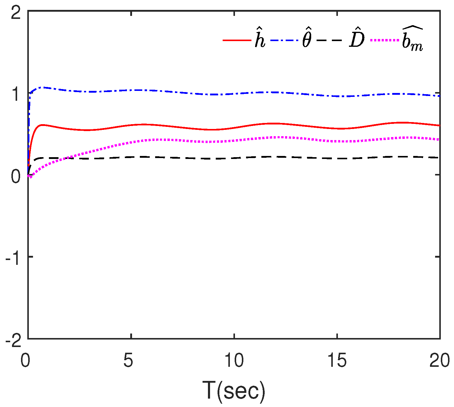
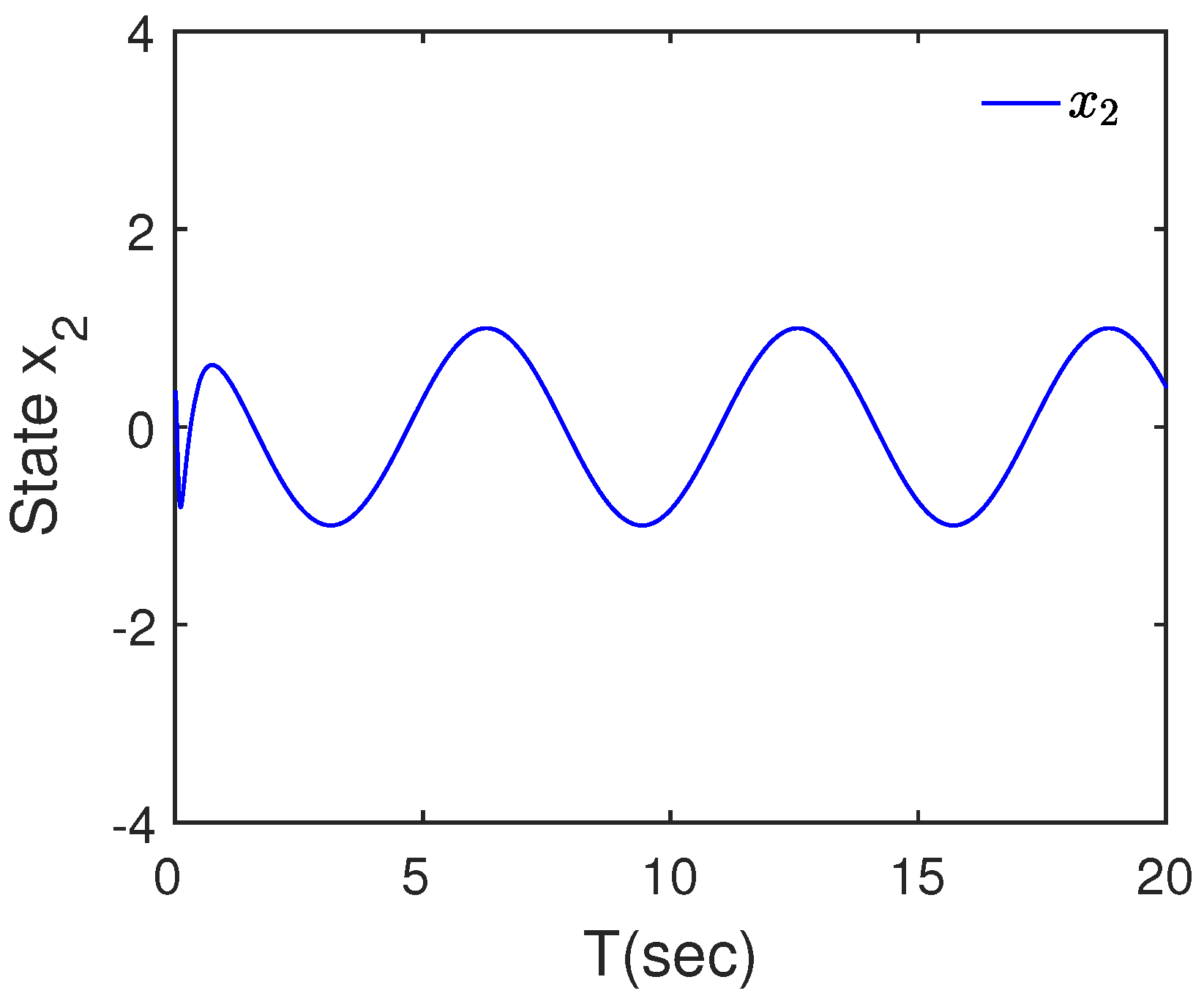
Figure 3 and Figure 4 show the system states $x_1,x_2$. Figure 3 and Figure 5 show the tracking performance, including the tracking error and the real-time dynamic tracking of the reference signal. Figure 6 shows the input signal of the dead-zone transformation. It is a control signal generated by the triggering mechanism shown in (75). Figure 7 shows the triggering time. Figure 8 shows the estimations of the unknown parameters. It is easy to see that all closed-loop signals are bounded.

With (64), the value of ${\hslash }_1$ is

$$\begin{array}{c}\hfill {\hslash }_1=max\left\{\frac{1}{2},\frac{5}{2},\frac{2}{0.4},\frac{1}{0.8},\frac{1}{0.8}\right\}=5\end{array}$$

Then, from (61), we obtain $0.1\le {\overline{l}}_D\le 0.2$ and $0.999\le {\overline{l}}_b\le 1$. With (66), we have

$$\begin{array}{c}\hfill {\hslash }_2=min\left\{7,8,0.1,0.05,\frac{1}{2}{\overline{l}}_D,\frac{1}{2}{\overline{l}}_b\right\}=0.05\end{array}$$

With (53), ${\Xi }_1$ can be calculated as

$$\begin{array}{ccc}\hfill {\Xi }_1& =& \frac{1}{2}\times 0.1\times {(0.5-1.2)}^2+\frac{1}{2}\times 0.2\times {(2.02-0.1)}^2+\frac{1}{2}\times {(2-0.8)}^2\hfill \\ & & +\frac{1}{2}\times 0.2\times {(2-0.2)}^2+0.1\times {\left(2(1+0.8)\right)}^2=2.73314\hfill \end{array}$$

From (59), we have

$$2.73314\le \Xi \le 2.73314+0.41204=3.14518$$

Then, we obtain

$$\sqrt{\frac{2{\hslash }_1}{{\hslash }_2}\Xi }=\sqrt{\frac{10}{0.05}2.73314}=23.3801$$

Obviously, the tracking error in the simulation meets this range.

Next, we consider that the external disturbance $d_e\left(t\right)=-6sin\left(t\right)+0.6$ exists in nonlinear systems (72). At the same time, the value of the unknown parameter is changed to 3. Thus, the system model can be expressed by

$$\begin{array}{ccc}\hfill {\dot{x}}_1& =& x_2+sin\left(x_1\right);\hfill \\ \hfill {\dot{x}}_2& =& 3(2+cos\left(x_1{x}_2\right))+u+d_e\left(t\right)\hfill \end{array}$$

(76)

The dead-zone input, auxiliary function $sg(·)$, and the triggering mechanism are chosen to be the same as in (73)–(75), respectively. The reference signal is taken as $y_r=sin\left(t\right)$. In the simulation, the design parameters are taken as $k_1=7,k_2=8$, ${\eta }_h=0.2$, ${\eta }_D=0.4$, ${\eta }_b=0.4$, $\Gamma =0.2$, $l_h=0.1$, $l_D=0.2$, $l_b=1$, $l_{\theta }=0.2$, $h_0=1.2$, ${\theta }_0=0.2$, $D_0=0.1$, $b_{m0}=0.8,{\epsilon }_i=0.1(i=0,1,2,3,4)$.

Figure 9 and Figure 10 show the system states $x_1,x_2$. Figure 9 and Figure 11 show the tracking performance, including the tracking error and the real-time dynamic tracking of the reference signal. Figure 12 is the input signal of the dead-zone transformation. It is a control signal generated by the triggering mechanism shown in (75). Figure 13 shows the triggering time. Figure 14 shows the estimations of unknown parameters. It is easy to see that all closed-loop signals are bounded, and the proposed control scheme has strong robustness against changes in unknown parameters and external disturbances.

(2) Secondly, we consider the following single-link rigid robot system [23]:

$$\begin{array}{c}\hfill J_r\ddot{\theta }=-\frac{1}{2}{m}_{r}g{l}_{r}sin\left(\theta \right)-M_{r}g{l}_{r}sin\left(\theta \right)+DI\left(v\right)\end{array}$$

(77)

where $0\le \theta \le \frac{\pi }{2}$ is the joint rotation angle. The value of the mass of the load is $m_r=1.5 \mathrm{kg}$. In addition, $g=9.8 \mathrm{m}/{\mathrm{s}}^2$ is a constant. The length of the robot link and the mass of the rigid link are taken as $l_r=0.5 \mathrm{m}$ and $M_r=3 \mathrm{kg}$, respectively. The moment of inertia is $J_r=M_r{l}_r^2+\frac{1}{3}{m}_r{l}_r^2$. $DI\left(v\right)$ represents the dead-zone input and can be described by

$$DI\left(v\right)=\left\{\begin{array}{cc}m(v-b_r)& v\ge b_r\\ 0& b_l<v<b_r\\ m(v-b_l)& v\le b_l\end{array}\right.$$

(78)

where $m=2$, $b_r=1,b_l=-0.8$. Letting $x_1=\theta$ and $x_2=\dot{\theta }$, the system model (77) can be rewritten as

$$\begin{array}{ccc}\hfill {\dot{x}}_1& =& x_2\hfill \\ \hfill {\dot{x}}_2& =& \frac{1}{J_r}(-\frac{1}{2}{m}_{r}g{l}_{r}sin\left(x_1\right)-M_{r}g{l}_{r}sin\left(x_1\right)+DI\left(v\right))\hfill \end{array}$$

(79)

In the simulation, the design parameters are selected as $k_1=7,k_2=8$, ${\eta }_h=0.1$, ${\eta }_D=0.4$, ${\eta }_b=0.05$, $l_h=0.1$, $l_D=0.2$, $l_b=1$, $h_0=1.2$, $D_0=0.1,b_{m0}=0.8$, ${\epsilon }_i=0.1(i=0,1,2,3,4)$. The reference signal is taken as $y_r=sin\left(t\right)$. The auxiliary function $sg(·)$ is the same as in (74). The triggering mechanism is

$$\begin{array}{c}{v}^T\left(t\right)=v\left(t_k\right),t\in [t_k,t_{k+1})\hfill \\ t_{k+1}=infimum\left\{t\in R:|v^e|\ge 0.5+0.2sin\left(t\right)\right\}\hfill \\ t_1=0\hfill \end{array}$$

(80)

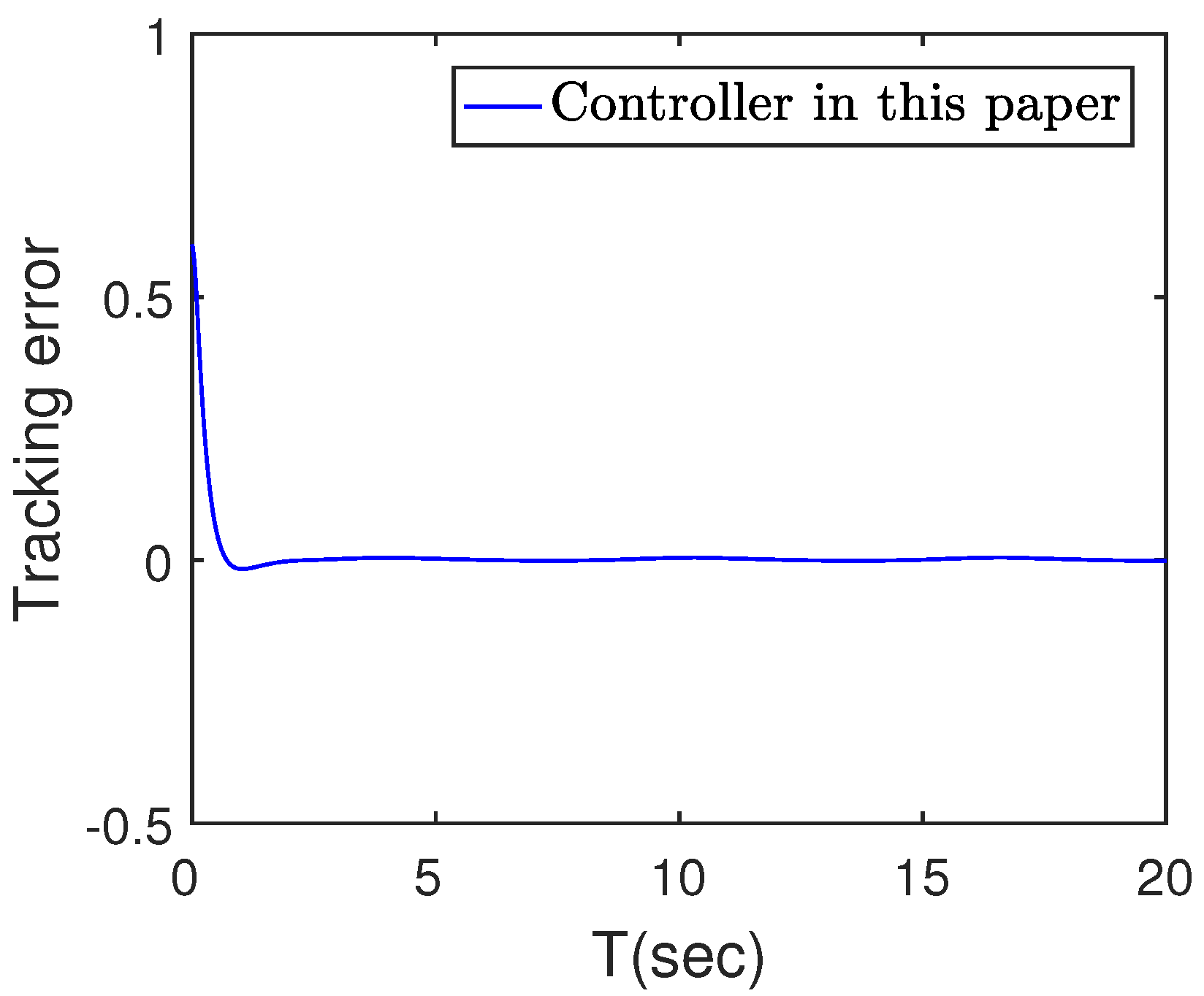
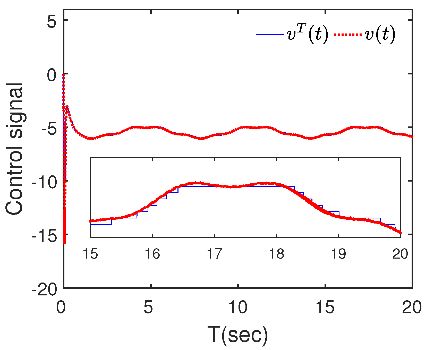
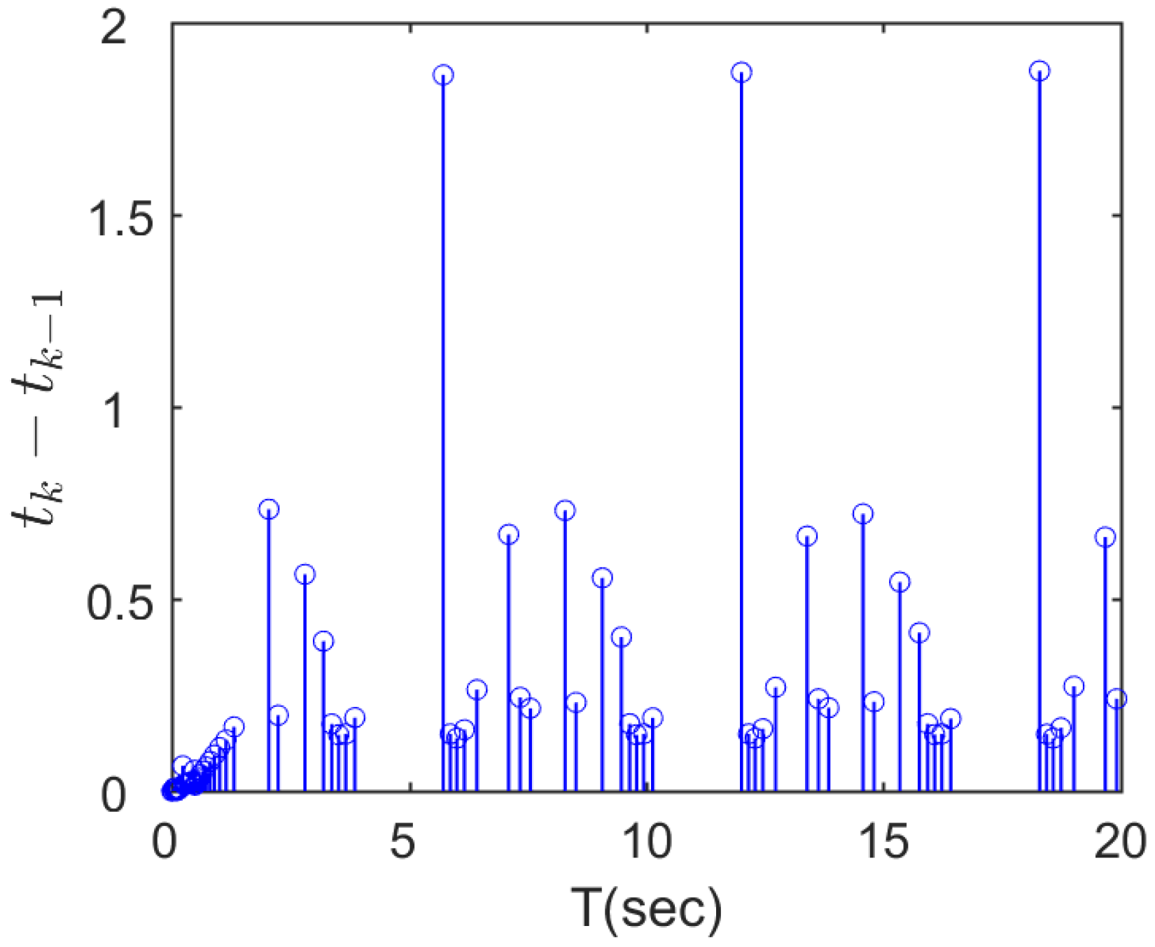
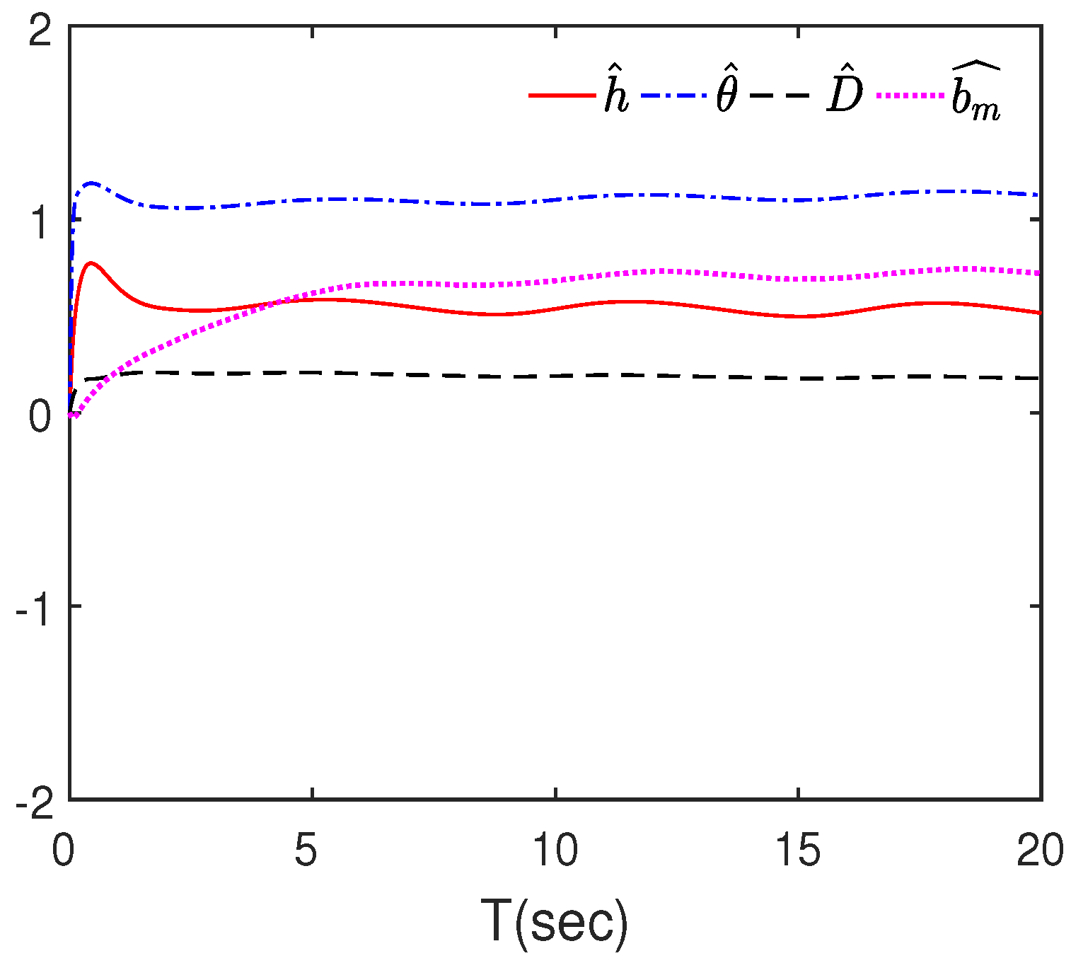
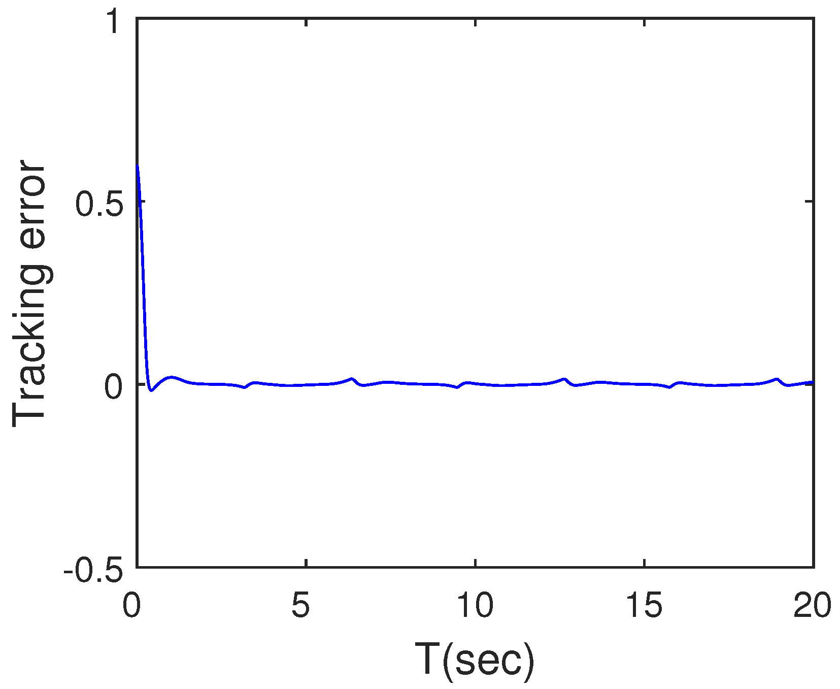
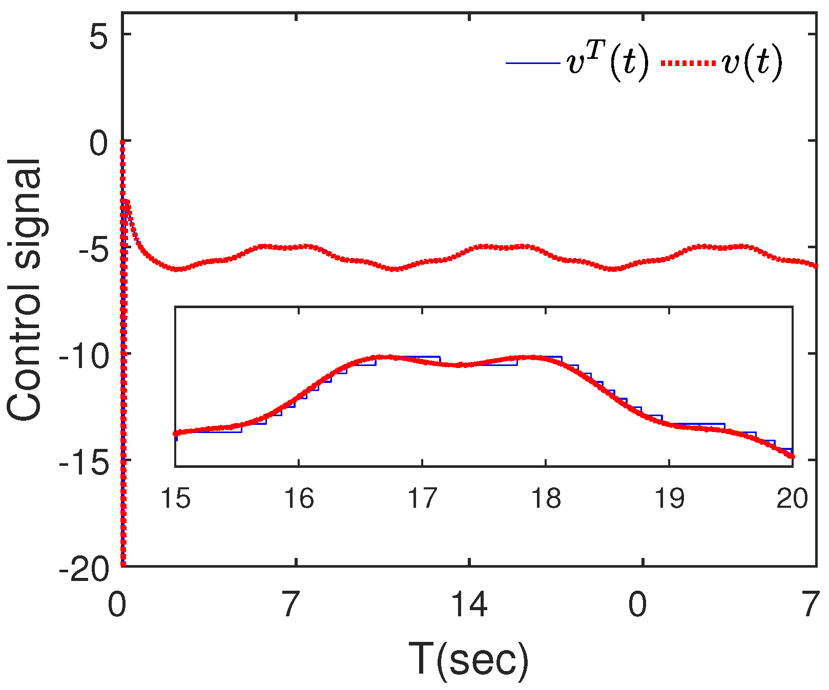
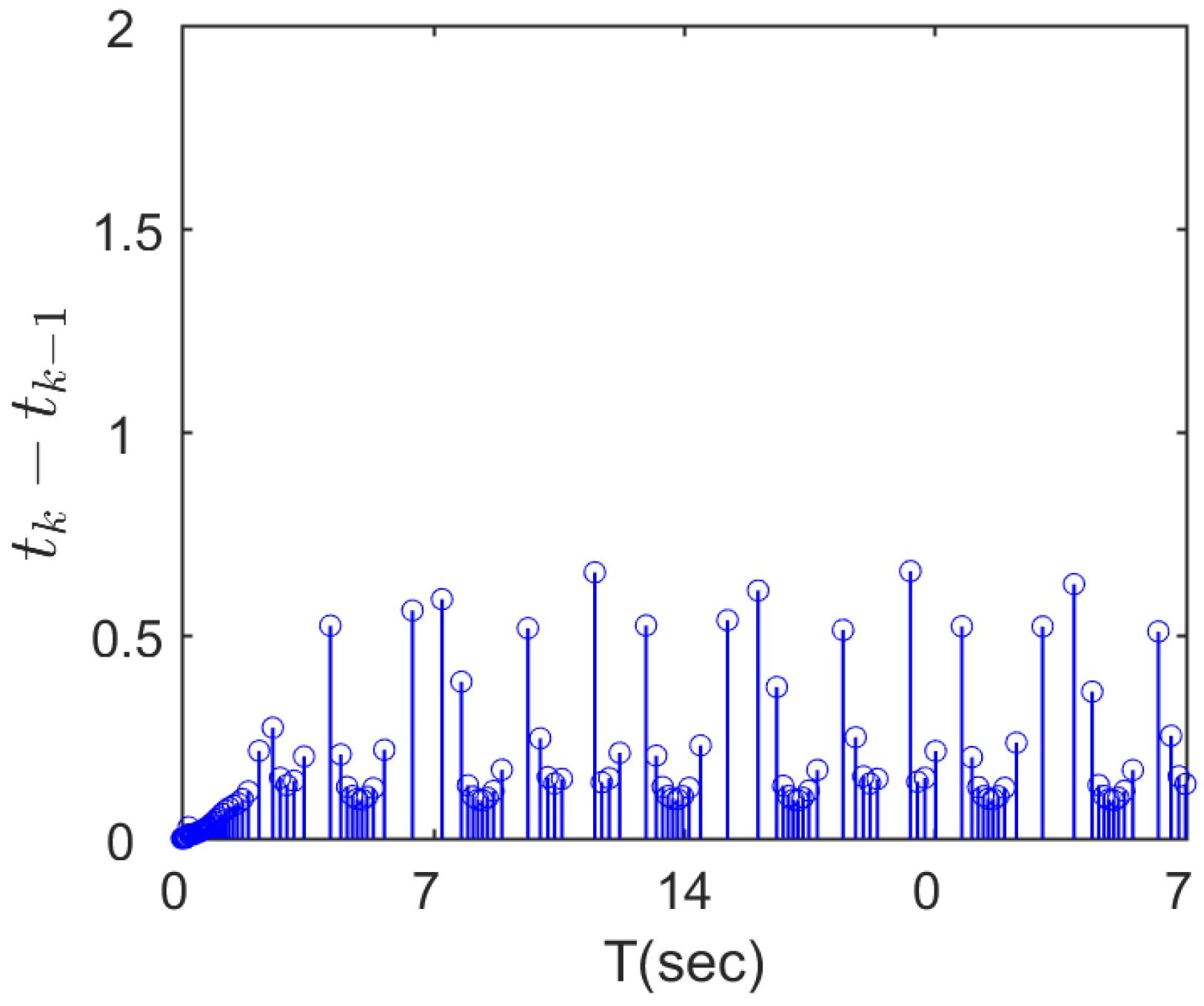
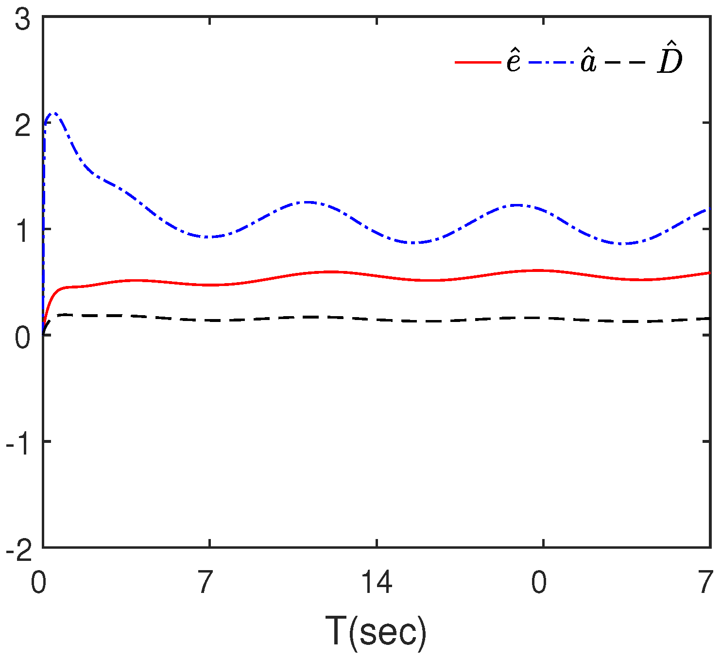
Figure 15 and Figure 16 show the system states $x_1,x_2$. Figure 15 and Figure 17 show the tracking performance, including the tracking error and the real-time dynamic tracking of the reference signal. Figure 18 shows the input signal of dead-zone transformation. It is a control signal generated by the triggering mechanism shown in (75). Figure 19 shows the triggering time. Figure 20 shows the estimations of unknown parameters. It is easy to see that all closed-loop signals are bounded.

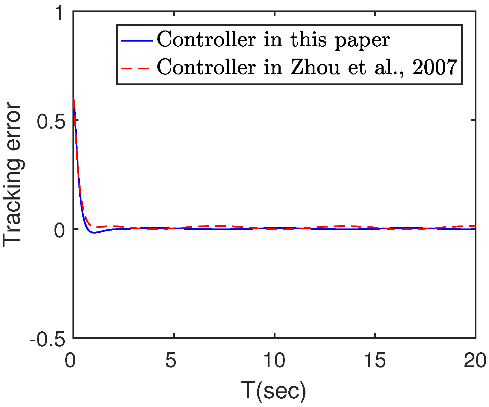
(3) Finally, for the second-order system shown in (72), we conducted simulations using the controller in [1] and the controller proposed in this paper, and compared and analyzed the simulation results. For fairness, the control input signal in [1] needs to be discretized through the same triggering mechanism before acting on the system. The system model can be described as

$$\begin{array}{ccc}\hfill {\dot{x}}_1& =& x_2+sin\left(x_1\right);\hfill \\ \hfill {\dot{x}}_2& =& (2+cos\left(x_1{x}_2\right))\theta +u\hfill \end{array}$$

(81)

The triggering mechanism is

$$\begin{array}{c}{v}^T\left(t\right)=v\left(t_k\right),t\in [t_k,t_{k+1})\hfill \\ t_{k+1}=infimum\left\{t\in R:|v^e|\ge 0.06+0.02sin\left(t\right)\right\}\hfill \\ t_1=0\hfill \end{array}$$

(82)

The other design parameters and initial values are the same as those in simulation (1). The dead-zone model, reference signal, and auxiliary function $sg\left(zn\right)$ are also the same as simulation (1).

Figure 21 and Figure 22 show the input signals generated by the proposed controller in this paper and by the controller in [1], respectively. Figure 23 and Figure 24 show the triggering times. The estimations of unknown parameters are given in Figure 25 and Figure 26. The comparison of tracking performance is shown in Figure 27, and the trigger times are shown in Figure 28. From the comparison of the simulation results, it can be seen that the controller proposed in this article can achieve better tracking performance with fewer communication times.

5. Conclusions

An event-triggered adaptive control scheme is proposed based on backstepping techniques for a class of nonlinear systems with unknown parameters, dead-zone input, and external disturbance. We not only consider the presence of external disturbances in the system but also introduce unknown disturbances in the design of the triggering mechanism. Then, a dynamic threshold with external disturbance is constructed. It is shown that the proposed adaptive control scheme can ensure all signals in the closed-loop system are bounded, and the tracking performance is also established. Finally, simulation studies are used to verify the effectiveness of the proposed scheme. The event-triggered control scheme presented in this paper is mainly designed for nonlinear systems with unknown dead-zone input. However, there are still some problems that need to be addressed. In the design of the event-triggered controller, a more general dead-zone input model should be considered, especially when the dead zone’s unknown parameters are time-varying. In addition, the triggering threshold should be related to the size of the control input. When the control input is large, the threshold should also correspondingly increase.

References

- Zhou, J.; Wen, C. Adaptive Backstepping Control of Uncertain Systems; Springer: Berlin/Heidelberg, Germany, 2007. [Google Scholar]
- Zhou, J.; Wen, C.; Zhang, Y. Adaptive output control of nonlinear systems with uncertain dead-zone nonlinearity. IEEE Trans. Autom. Control. 2006, 51, 504–511. [Google Scholar] [CrossRef]
- Zong, G.; Wang, Y.; Karimi, H.R.; Shi, K. Observer-based adaptive neural tracking control for a class of nonlinear systems with prescribed performance and input dead-zone constraints. Neural Netw. 2022, 147, 126–135. [Google Scholar] [CrossRef] [PubMed]
- Liu, M.; Zhang, W.; Ma, L. Finite-time adaptive fuzzy control for a class of output constrained nonlinear systems with dead-zone. Int. J. Adapt. Control. Signal Process. 2022, 36, 69–87. [Google Scholar] [CrossRef]
- Yao, D.; Dou, C.; Zhao, N.; Zhang, T. Finite-time consensus control for a class of multi-agent systems with dead-zone input. J. Frankl. Inst. 2021, 358, 3512–3529. [Google Scholar] [CrossRef]
- Zhang, G.; Yao, M.; Zhang, W.; Zhang, W. Improved composite adaptive fault-tolerant control for dynamic positioning vehicle subject to the dead-zone nonlinearity. IET Control. Theory Appl. 2021, 15, 2067–2080. [Google Scholar] [CrossRef]
- Jia, X.; Xu, S.; Shi, X.; Zhang, Z. Global practical tracking for nonlinear systems with uncertain dead-zone input via output feedback. J. Frankl. Inst. 2021, 358, 2987–3009. [Google Scholar] [CrossRef]
- Jiang, B.; Gao, C. Decentralized adaptive sliding mode control of large-scale semi-markovian jump interconnected systems with dead-zone input. IEEE Trans. Autom. Control. 2022, 67, 1521–1528. [Google Scholar] [CrossRef]
- Krstic, M.; Kanellakopoulos, I.; Kokotovic, P.V. Nonlinear and Adaptive Control Design; Wiley: New York, NY, USA, 1995. [Google Scholar]
- Zhu, Y.; Su, H.; Krstic, M. Adaptive backstepping control of uncertain linear systems under unknown actuator delay. Automatica 2015, 54, 256–265. [Google Scholar] [CrossRef]
- Lai, G.; Liu, Z.; Zhang, Y.; Chen, C.L.P.; Xie, S. Adaptive backstepping-based tracking control of a class of uncertain switched nonlinear systems. Automatica 2018, 91, 301–310. [Google Scholar] [CrossRef]
- Yang, D.; Gao, X.; Cui, E.; Ma, Z. State-constraints adaptive backstepping control for active magnetic bearings with parameters nonstationarities and uncertainties. IEEE Trans. Ind. Electron. 2020, 68, 9822–9831. [Google Scholar] [CrossRef]
- Aslmostafa, E.; Ghaemi, S.; Badamchizadeh, M.A.; Ghiasi, A.R. Adaptive backstepping quantized control for a class of unknown nonlinear systems. Isa Trans. 2022, 125, 146–155. [Google Scholar] [CrossRef] [PubMed]
- Xing, L.; Wen, C.; Liu, Z.; Su, H.; Cai, J. Event-triggered adaptive control for a class of uncertain nonlinear systems. IEEE Trans. Autom. Control. 2017, 62, 2071–2076. [Google Scholar] [CrossRef]
- Xing, L.; Wen, C.; Liu, Z.; Su, H.; Cai, J. Adaptive compensation for actuator failures with event-triggered input. Automatica 2017, 85, 129–136. [Google Scholar] [CrossRef]
- Xing, L.; Wen, C.; Liu, Z.; Su, H.; Cai, J. Event-triggered output feedback control for a class of uncertain nonlinear systems. IEEE Trans. Autom. Control. 2019, 64, 290–297. [Google Scholar] [CrossRef]
- Choi, Y.H.; Yoo, S.J. Decentralized event-triggered tracking of a class of uncertain interconnected nonlinear systems using minimal function approximators. IIEEE Trans. Syst. Man, Cybern. Syst. 2019, 51, 1766–1778. [Google Scholar] [CrossRef]
- Hu, Y.; Liu, W. Adaptive fuzzy dynamic surface control for nonstrict-feedback nonlinear state constrained systems with input dead-zone via event-triggered sampling. Appl. Math. Comput. 2023, 450, 1–17. [Google Scholar] [CrossRef]
- Wu, L.; Park, J.H.; Xie, X.; Liu, Y.; Yang, Z. Event-triggered adaptive asymptotic tracking control of uncertain nonlinear systems with unknown dead-zone constraint. Appl. Math. Comput. 2020, 386, 1–13. [Google Scholar] [CrossRef]
- Su, X.; Liu, Z.; Lai, G. Event-triggered robust adaptive control for uncertain nonlinear systems preceded by actuator dead-zone. Nonlinear Dyn. 2018, 93, 219–231. [Google Scholar] [CrossRef]
- Yu, Q.; He, X.; Wu, L.; Guo, L. Finite-time command filtered event-triggered adaptive output feedback control for nonlinear systems with unknown dead-zone constraints. Inf. Sci. 2022, 617, 482–497. [Google Scholar] [CrossRef]
- Wang, C.; Wang, J.; Zhang, C.; Du, Y.; Liu, Z.; Chen, C.L.P. Fixed-time event-triggered consensus tracking control for uncertain nonlinear multiagent systems with dead-zone constraint. Int. J. Robust Nonlinear Control. 2023, 33, 6151–6170. [Google Scholar] [CrossRef]
- Li, H.; Zhao, S.; He, W.; Lu, R. Adaptive finite-time tracking control of full state constrained nonlinear systems with dead-zone. Automatica 2019, 100, 99–107. [Google Scholar] [CrossRef]
- Yue, H.; Feng, S.; Li, J. Event-triggered adaptive control for stochastic nonlinear systems with time-varying full state constraints and output dead-zone. J. Frankl. Inst. 2023, 360, 11965–11994. [Google Scholar] [CrossRef]
- Máarif, A.; Márquez-Vera, M.A.; Mahmoud, M.S.; Ladaci, S.; Cakan, A.; Nino-Parada, J. Backstepping sliding mode control for inverted pendulum system with disturbance and parameter uncertainty. J. Robot. Control. 2022, 3, 86–92. [Google Scholar] [CrossRef]
Figure 1.
The block diagram.
Figure 2.
The block diagram about the closed-loop feedback system.
Figure 3.
Output signal .
Figure 4.
State .
Figure 5.
Tracking error.
Figure 6.
Input signal v.
Figure 7.
Triggering time.
Figure 8.
Estimations of parameters.
Figure 9.
Figure 10.
Figure 11.
Figure 12.
Figure 13.
Figure 14.
Figure 15.
Figure 16.
Figure 17.
Figure 18.
Figure 19.
Figure 20.
Figure 21.
Input v (this paper).
Figure 22.
Input v (reference [1]).
Figure 23.
Time (this paper).
Figure 24.
Time (reference [1]).
Figure 25.
Estimations (this paper).
Figure 26.
Estimations (reference [1]).
Figure 27.
Tracking error [1].
Figure 28.
Communications [1].