

A New Safety Distance Model Based on Braking Process Considering Adhesion Coefficient

School of Computer Science and Engineering, Xi’an University of Technology, Xi’an 710048, China
*
Author to whom correspondence should be addressed.
Electronics 2024, 13(2), 421; https://doi.org/10.3390/electronics13020421
Submission received: 21 August 2023
/
Revised: 6 October 2023
/
Accepted: 24 October 2023
/
Published: 19 January 2024
(This article belongs to the Section Electrical and Autonomous Vehicles)
Abstract
:The traditional safety distance model based on the braking process is inadequate for scenarios where the adhesion coefficient varies. This research presents a safety distance model that takes into account the real-time fluctuations in the adhesion coefficient during the braking process. The proposed safety distance model is the basis for a three-level control strategy aimed at ensuring the safety and stability of the car-following process. A simulation is conducted to model the variation of the road’s adhesion coefficient during car braking. The experimental results, obtained for various initial adhesion coefficients and speeds, demonstrate that the precision of the safety distance calculated is improved by a minimum of 14.99% when compared to the traditional safety distance. Furthermore, the simulation results of the car-following process of a motorcade consisting of five cars provide evidence of the safety and stability of the suggested model.
1. Introduction
The current state of affairs is that traffic flow models can be classified into three distinct categories according to their level: microscopic, mesoscopic, and macroscopic [1,2]. When compared to the macroscopic and mesoscopic traffic flow models, the microscopic traffic flow model can provide a more detailed description of the car-following motion state. Furthermore, the car-following model is considered to be the foundation of the microscopic traffic flow model [3].
The car-following model, which includes the most fundamental microscopic driving behavior, is the subject of research [4]. The interaction between two neighboring vehicles in a vehicle fleet that does not permit passing is the most basic microscopic driving behavior. This model describes the interaction between two adjacent vehicles in a vehicle fleet that is traveling on a single-lane road and does not allow overtaking [5,6,7]. There are six different types of car-following models that are commonly used. These models include the data-driven model, the stimulus−response model, the physiological and psychological models, the safety distance model, and the cellular automata model.
In order to investigate the impact that the conditions under which cars are driven have on the flow of traffic, Kometani et al. [8] computed the safe following distance by utilizing the speed of the front and rear cars and suggested the safety distance model for the very first time.
According to the safety distance model, the following automobile is required to maintain a safety distance from the leading car by adjusting the speed while driving. This is carried out in order to prevent the following car from colliding with the leading car in the event of a sudden braking [9]. The Gipps model was developed in 1981, taking into account the various aspects that have an impact, such as the acceleration constraint and the safety distance constraint. This model eliminates the issue that arises from an inconsistent reaction time during the simulation process [10]. In [11], a safety distance warning system is proposed to warn drivers to avoid collision accidents in dangerous conditions. This system measures the distance between the leading vehicle (obstacle) and the following car and then determines the safety distance of the following car. To explicitly calculate the minimum safe car-following distance, a new method is proposed in [12]. This method involves analyzing the kinematics of the vehicles involved that are involved in the car-following process. This method has the ability to identify the behavioral characteristics of the car-following driver and measure the safety distance in the car-following regime. To enhance the accuracy of traditional safety distance models, which are based on the braking process of the leading vehicle, a new safety distance model is established by considering the changing process of deceleration. This model is based on traditional safety distance models and uses a one-lane following condition. The goal of this model is to improve the accuracy of the safety distance [13].
The traditional safety distance models are categorized into three groups based on their theories: headway, the braking process, and the driver model [14]. An inherent limitation of the safety distance model that relies on headway is that it calculates a very small safety distance when there is a significant difference in speed, thereby failing to ensure safety. Conversely, the primary drawback of the safety distance model based on the driver model is the challenge of incorporating all drivers’ driving characteristics into a single model. The safety distance model which relies on the braking process guarantees the driving safety of cars equipped with braking control systems in dangerous conditions [15,16].
The safety distance is intricately linked to the braking procedure. The braking distance is significantly influenced by the surface type, as different surfaces have varying coefficients of adhesion [17]. A novel safety distance model is introduced to enable the car to adjust to various driving conditions based on the adhesive coefficient, while also aligning with drivers’ characteristics in terms of driving intention [18]. Sevil introduces an algorithm in [19] that incorporates the adhesion coefficient into the adaptive AEB system. This algorithm adjusts the timings of the collision alert warnings and emergency braking based on the adhesion coefficient. The method presented in [20] integrates vehicle dynamics and tire normal force variation. It utilizes the least square method for multivariate fitting, based on the slip ratio and adhesion coefficient. This approach establishes the relationship between the rolling resistance coefficient and road adhesion coefficient. The relationship between rolling resistance coefficient and road adhesion coefficient is determined in [20], using the slip ratio and adhesion coefficient as the basis. Furthermore, numerous studies in the existing literature employ a Kalman filter to estimate the adhesion coefficient of the road [21]. However, it is not possible to guarantee the complete accuracy of the estimated friction coefficient in real time [22]. The vehicle–infrastructure cooperation (VIC) system, which allows for communication between vehicles and roads, has been made possible by the rapid advancement of communication technology. This system enables the transfer of real-time information such as the position, speed, acceleration, and other driving details between vehicles and roads [23,24]. In this study, we assume that the adhesion coefficient information of the driving road is already known, and the adhesion coefficient of the road section only needs to be determined based on the car’s position. Real-time information, such as the speed and position of cars, can be obtained through an intelligent transportation system [25].
The car-following model has an impact on the stability of traffic flow, which is crucial for determining the level of organization in the traffic stream [26]. Driven by the significant impact on safety, dependability, and effectiveness, the stability of traffic has been thoroughly and extensively investigated [27]. In their study, D. Ngoduy et al. [28] examined the stability of traffic flow in the presence of mixed traffic by analyzing the variations in head spacing. In their study, M. Wang et al. [29] introduced a delay compensation strategy for automatic driving stability control and demonstrated its efficacy. Y. Li et al. [30] employed the Lyapunov approach to rigorously examine the convergence of the delay-dependent system, thereby guaranteeing the stability of the system.
The traditional safety distance model, which solely takes into account the adhesion coefficient of the road where both the leading and the following car are situated during the braking process, is inadequate for the scenario involving varying adhesion coefficient. Considering the real-time variation in the adhesion coefficient, we proposed a novel safety distance model that takes into account the dynamic changes in the adhesion coefficient throughout the braking process. Based on this, three safety distances are calculated to efficiently implement the control strategy of the subsequent vehicle. The theoretical analysis is performed utilizing the Lyapunov stability theorem. Subsequently, the efficacy of the proposed model is validated by analyzing the simulation results of the scenario where the adhesion coefficient varies during car braking. Furthermore, the safety and stability of the proposed model is demonstrated through modeling the car-following process of a motorcade of five cars.
The paper presents several key contributions:
- We introduce a novel safety distance model that takes into account the real-time changes in the adhesion coefficient during the braking process. Simulation results demonstrate that this model improves the accuracy of calculated safety distance by at least 14.99% compared to traditional methods.
- We analyze the entire reaction braking process and find that the traditional safety distance model fails to ensure overall safety.
- The proposed model’s safety and stability are validated through simulation of a car-following process involving a motorcade of five cars.
The rest of the paper is divided into four sections. In Section 2, we primarily present the traditional safe distance model. Section 3 introduces a novel safety distance model that takes into account the real-time changes in the adhesion coefficient adhesion coefficient during the braking process. The suggested model is evaluated by simulating the changes in the adhesion coefficient of the road during car braking in Section 4. Furthermore, simulation results of the car-following process provide evidence of the safety and stability of the proposed model. The conclusions of this investigation are presented in Section 5.
2. Preliminaries
2.1. Description of Parameters
The symbols as well as the description of relevant parameters are presented in Table 1.
2.2. Traditional Safety Distance Model
During the process of car following, it is essential to maintain a specific safety distance between the preceding vehicle and the subsequent vehicle. The safety distance model aims to ensure a sufficient spacing between vehicles to prevent rear-end collisions when the leading vehicle suddenly brakes [31]. The leading car abruptly applies its brakes with the highest possible rate of deceleration at time , continues to travel at its initial speed, then applies its brakes with the highest possible rate of deceleration after a reaction time, after reaction time , until the speed of the rear car reaches zero at time . Calculation of is represented by Equation (1).
The total distance traveled by the car from to consists of the response distance and braking distance . Equations (2) and (3) illustrate the computation of reaction distance and braking distance respectively. The distance traveled by the leading car during its braking is , it is calculated as shown in Equation (4).
where and are the positions of the leading car and the following car, and are the maximum deceleration of the following car and the leading car at time t, respectively.
The traditional minimum safety distance is:
where is the length of car n, is the static safety distance.
The relationship between the maximum deceleration and the adhesion coefficient of the road is shown in Equation (6).
where is the adhesion coefficient of the road, is the acceleration of gravity.
Therefore, the minimum safety distance is shown in Equation (7).
3. Proposed Safety Distance Model
3.1. Proposed Safety Distance
3.1.1. Minimum Safety Distance
Equation (7) shows that in the conventional safety distance model, on the road where the leading car and the following car are presently situated, the adhesion coefficient fluctuates during the braking process. Equation (7) demonstrates that the traditional safety distance model, which solely takes into account the adhesion coefficient of the road where the leading car and the following car are currently located, is inadequate for situations where the adhesion coefficient changes during the cars’ braking process.
Equation (8) displays the adhesion coefficient of the road, given that there is a sufficiently long road with various road conditions.
where is the coordinate, is the starting coordinate of road section , is the ending coordinate of road section , is the adhesion coefficient of road section , and is the total number of road sections.
Assuming that the car n on the road applies the maximum deceleration of each section at time and the velocity reaches zero at time , let us assume that the car is in section at time and section at time , as shown in Equations (9) and (10).
The braking process of the car is shown in Figure 1.
In case Equation (11) is not satisfied, . This degenerates into a single road condition suited for the standard safety distance paradigm. Therefore, we just evaluate Equation (11). In this case, , can be obtained from Equation (12).
where is the speed at which the car n reaches section during braking, and its calculation is shown in Equation (13).
And the calculation of the time when the car n arrives at section is shown in Equation (14).
The calculation of is shown in Equation (15).
The calculation for the distance traveled when braking is as follows. If the car n brakes at the maximum deceleration of each section from time , the distance traveled up to time is calculated as shown in Equation (16).
In Equation (16), the value range of in condition is . The traveling distance during reaction and braking is calculated as follows. Starting from time , the car n first travels at a constant initial speed within the reaction time , and then brakes at the maximum deceleration of each section. The distance traveled up to time t is calculated as shown in Equation (17).
The minimum safety distance proposed in this paper is:
The value range of in Equation (18) is shown in Equation (19).
3.1.2. Expected and Maximum Safety Distance
The expected safety distance, as described by reference [32], is the sum of the minimum safety distance and the reaction distance. Equation (20) demonstrates the computation of the anticipated safety distance.
The maximum safety distance is defined as the distance that the car travels at the maximum speed for a reaction time plus the expected safety distance, as shown in Equation (21).
where is the maximum allowable driving speed on the road.
3.2. The Control Strategy of Proposed Car-Following Model
The control strategy of the following car is affected by both the distance and the safety distance between the leading car and the following car. The distance between the leading car and the following car is calculated as shown in Equation (22).
The control strategy of the following car is: when the distance is less than the minimum safety distance , the following car decelerates at its maximum deceleration to ensure safety; when is greater than or equal to , the following car accelerates according to the relationship between and ; when is greater than or equal to and less than , the following car adjusts the speed according to , , , and . The control strategy of the following car is shown in Equation (23).
where is the maximum comfortable acceleration of the following car, the adjustment factor is a positive constant, the step function is shown in Equation (24).
According to Equations (23) and (24), the range of is .
3.3. The Stability Analysis
The main issue in the study of traffic dynamics is the stability of traffic dynamics. The fundamental concept is that when the motorcade operates smoothly, the disruptions generated by the leading car are progressively less as they propagate towards the rear of the motorcade. Given that the automobile’s following speed is and the distance between adjacent car is when the motorcade runs stably, the steady-state position of car can be expressed by Equation (25).
The weak interference of the leading car at time can be expressed by Equation (26).
where is the actual position of car at time , is the eigenvalue, and is the Fourier expansion parameter, as shown in Equation (27).
Equations (28) and (29) can be obtained from Equation (26).
According to Equation (22), when the leading car experiences a small disturbance, the acceleration of the following car is determined by the difference in speed and position between the two cars. Furthermore, the vehicle-following model is usually described by a delay differential equation [33]. Various car-following models, such as the GHR model, take into account the impact of the velocity and distance between two cars on the acceleration of the following car. To streamline the analysis, let us denote , a linearized form of the equation, as Equation (30).
where , , and are shown in Equations (31)–(33). , , and can be obtained by Equations (34)–(36), respectively.
The Taylor expansion of is shown in Equation (37), and the eigenvalue can be expressed by Equation (38).
According to Equations (26) and (30)–(38), and are shown in Equations (39) and (40), respectively.
If the second order coefficient of eigenvalue is negative, the model is considered unstable. Otherwise, the model is stable. The stability criteria of the model are shown in Equation (41).
4. Results and Discussion
4.1. Comparison with Traditional Safety Distance
The safety distance is primarily influenced by the velocity of both the leading and the following vehicles, the coefficient of adhesion, the response time, the length of the vehicles, and static safety distance. In this study, reaction time is 1 s, the static safety distance is 5 m, the length of cars is 4 m. We analyze the optimal separation distance for various combinations of velocity and adhesion coefficient.
A simulation is conducted to model the variation of adhesion coefficient during car braking considering a sufficiently a long road and . At time t, the leading car performs emergency braking at its maximum deceleration until the speed drops to zero at coordinate ; the following car keeps running at the original speed first, and then brakes at the maximum deceleration at coordinate after the reaction time until the speed drops to zero at coordinate . The coordinates , , and are shown in Equations (42)–(44), correspondingly.
The value range of is 0.1 to 0.9. The value range of is shown in Equation (45).
Let be 0 m. According to the combination of , , and , the parameter settings of the simulation scenes are shown in Table 2.
TSD represents the traditional minimum safety distance, and PSD represents the proposed minimum safety distance. For these six scenes, we calculate TSD, PSD, and TSD-PSD under various values of and . Taking scene 1 as an example, , , , . It can be divided into five cases according to the value of .
Case 1: .
Case 2: .
Case 3: .
Case 4: .
Case 5: .
The calculated TSD, PSD, and difference in scene 1 are shown in Figure 2, Figure 3, and Figure 4, respectively.
For cases 1 to 5, is , , , , and , respectively, is , , , , and , respectively.
For case 1, with the decrease in , the braking distances of the leading car and the following car increase, and since is greater than , the braking distance of the following car increases more, so TSD increases.
For cases 2 to 4, the braking distance of the following car is independent of in the traditional safe distance model. With the decrease in , the braking distance of the leading car increases, so TSD decreases. And for cases 2 to 4, the change in has no effect on the braking distance of the leading car.
For case 5, the braking distances of the leading car and the following car are independent of in the traditional safe distance model. Therefore, TSD remains unchanged.
It can be seen from Figure 2 that TSD changes sharply when is or . Let denote . When changes from to , the braking distance of the following car changes from to . In scene 1, is 100 m. When is 0.1, is 200 m, TSD decreases by 100 m due to the change in ; when is 0.9, is 22.22 m, so TSD increases by nearly 87.78 m due to the change in . When changes from to , the braking distance of the leading car changes from to . In scene 1, is 25 m. When is 0.1, is 50 m, so TSD increases by 25 m due to the change in ; when is 0.9, is 5.56 m, so TSD decreases by nearly 19.44 m due to the change in .
The calculated PSD in scene 1 is shown in Figure 3.
For cases 1, 3, and 5, during the braking process of the leading car and the following car, the adhesion coefficient does not change. Therefore, TSD and PSD are equal.
For case 2, the adhesion coefficient changes during the braking process of the following car. With the decrease in , the braking distances of the leading car and the following car increase. The braking distance of the leading car is independent of . When and the larger the , the less the braking distance of the following car increases; when and the larger the , the less the braking distance of the following car decreases.
When the value of is small, the braking distance of the following car has a greater impact on PSD than the braking distance of the leading car. As , increases, the impact of the braking distance of the following car on PSD steadily diminishes. Table 3 presents several combinations of and . Assuming a constant adhesion coefficient, the leading car’s braking distance is 25 m, while the following car’s braking distance is 100 m. When is 0.9 and 0.1, the braking distance of the leading car decreases by 19.44 m and increases by 25 m, respectively. The braking distance of the leading automobile changes by −77.62 m, −0.15 m, 99.8 m, and 0.21 m for combinations 1 to 4, respectively. The PSD changes are as follows: −58.18 m, 19.29 m, 74.8 m, and −24.79 m, respectively.
In scenario 5, the adhesion coefficient undergoes variations while the leading automobile is braking. The braking distance of the leading car remains constant, which does not impact the PSD. Therefore, the PSD is solely influenced by the braking distance of the leading car. As lowers, the braking distance of the leading car increases and the PSD decreases. Moreover, as the value of increases, the rate at which the safety distance increases falls and the rate at which the PSD reduces also decreases.
Figure 4 illustrates the computed difference between TSD and PSD in scene 1.
In scene 2, the braking distances of the following car are not affected by in the traditional safe distance model. However, in reality, the adhesion coefficient changes from to at as the pursuing car brakes. In the traditional safe distance model, the braking distances of the leading automobile in case 5 are not affected by . However, in reality, as the leading automobile brakes, the adhesion coefficient changes from to at . For examples 2 and 5, the smaller the value of or the greater the difference between and , the greater the difference between TSD and PSD.
For case 2, the difference between TSD and PSD is less than zero when . This is due to the fact that the braking distance of the following car calculated in the traditional safety distance is less than the actual value. On the other hand, when , the difference is greater than zero because the braking distance of the following car calculated in the traditional safety distance model is greater than the actual value.
In case 5, where , the difference between TSD and PSD is positive. This is because the calculated braking distance of the leading car in the traditional safety distance model is less than the actual value. Conversely, when , the difference is negative. This is because the calculated braking distance of the following car in the traditional safety distance model is greater than the actual value.
Given that has values of 0.1 and 0.9, and is 20.1 m, the reaction braking process of the following car is illustrated in Figure 5 and Figure 6, correspondingly.
Figure 5 and Figure 6 demonstrate that the adhesion coefficient changes from to at . However, the traditional safety distance model continues to compute the braking distance of the trailing vehicle based on . The traditional safety distance model fails to account for the changes in the adhesion coefficient throughout the braking phase of the following car. Consequently, this results in an erroneous estimation of the braking distance of the trailing vehicle, leading to inaccuracies in the calculation of the traditional safety distance. In Figure 5, the braking distance of the following car calculated in the traditional safety distance model is smaller than the actual one, indicating that traditional safety distance (TSD) is larger than actual safety distance (PSD) because < . In Figure 6, the braking distance of the following car calculated in the traditional safety distance model is larger than the actual one, indicating that TSD is smaller than PSD because > .
The accuracy improvement of the calculated safety distance can be determined by calculating the TSD and PSD for each combination of distinct values of and , and then finding the average value of . The simulation findings for scenes 1 to 6 demonstrate an improvement in the accuracy of the computed safety distance by 29.74%, 19.17%, 26.61%, 14.99%, 53.72%, and 32.42%, respectively, as compared to the traditional safety distance. The precision of the computed safety distance calculated is enhanced by a minimum of 14.99% as compared to the traditional safety distance.
4.2. Analysis of Car-following Process
To validate the safety and stability of the proposed car-following model, which is based on the brake safety distance, we simulate the driving scenarios of the motorcade during the following process. Consider a motorcade consisting of five cars, awaiting the green signal to proceed. The cars in the motorcade are immobile, with a 10-m gap between each adjacent car, and each car is 4 m in length. The first car initially accelerates uniformly with an acceleration of for a duration of 10 s, and subsequently maintains a constant velocity of . At the 70th second, the first car undergoes maximal deceleration until it reaches a complete stop. The following cars adhere to the control strategy of the car-following model.
4.2.1. Stability Analysis
From the 10th until the 70th second, the first car maintains a steady speed of 20 . As a result of the control strategy, the cars in the motorcade gradually synchronize their speeds over time, resulting in each car maintaining the same speed and equal distances between neighboring cars. The system achieves a state of stability. Figure 7 displays the velocity profile of each vehicle in the motorcade.
The system achieves stability at 62.29 s, 56.90 s, 43.76 s, 42.11 s, and 47.92 s when takes the values of 1, 1.5, 2, 2.5, and 3, respectively. Based on Figure 7, a small value of results in a control strategy that is not responsive to the errors in speed and the distance between adjacent cars. Consequently, the system’s ability to achieve a stable state is diminished. Therefore, for the values of equal to 1 and 1.5, the system takes longer to reach the stable state compared to when is 2, 2.5, and 3.
The average errors of the velocity and the distance between consecutive vehicles from the 50th to 70th seconds are as shown in Table 4.
For values of equal to 1, 1.5, 2, 2.5, and 3, the average error of the speed is 0.0176, 0.0073, 0.0013, 0.0009, 0.0023 , respectively. Similarly, the average error in the distance between adjacent cars is 0.0882, 0.0365, 0.0067, 0.0039, 0.0107 , accordingly. Table 4 indicates that selecting as 2.5 results in a faster attainment of system stability as well as reduced average errors in speed and distance. Consequently, the system exhibits improved stability. When the value of is 2.5, the motorcade reaches a stable condition after the first car moves at a constant speed for 32.11 s.
4.2.2. Safety Analysis
At the 70th second, the first car undergoes the maximum deceleration until it reaches a complete stop. In Figure 8, the distance between adjacent cars in the motorcade is shown at = 2.5. Figure 8 illustrates the distance between car n and car n + 1.
Figure 8 illustrates that, starting from the 70th second, the following cars experience deceleration as a result of the control strategy triggered by the emergency braking of the leading car. The first car comes to a stop at the 74th second followed by cars 2, 3, 4, and 5 successively reaching a stationary state at 82.58 s, 86.84 s, 90.02 s, and 98.42 s, respectively. Once the following car enters a stationary state, there is a slightly greater distance between this car and the leading car, exceeding the minimum safety distance.
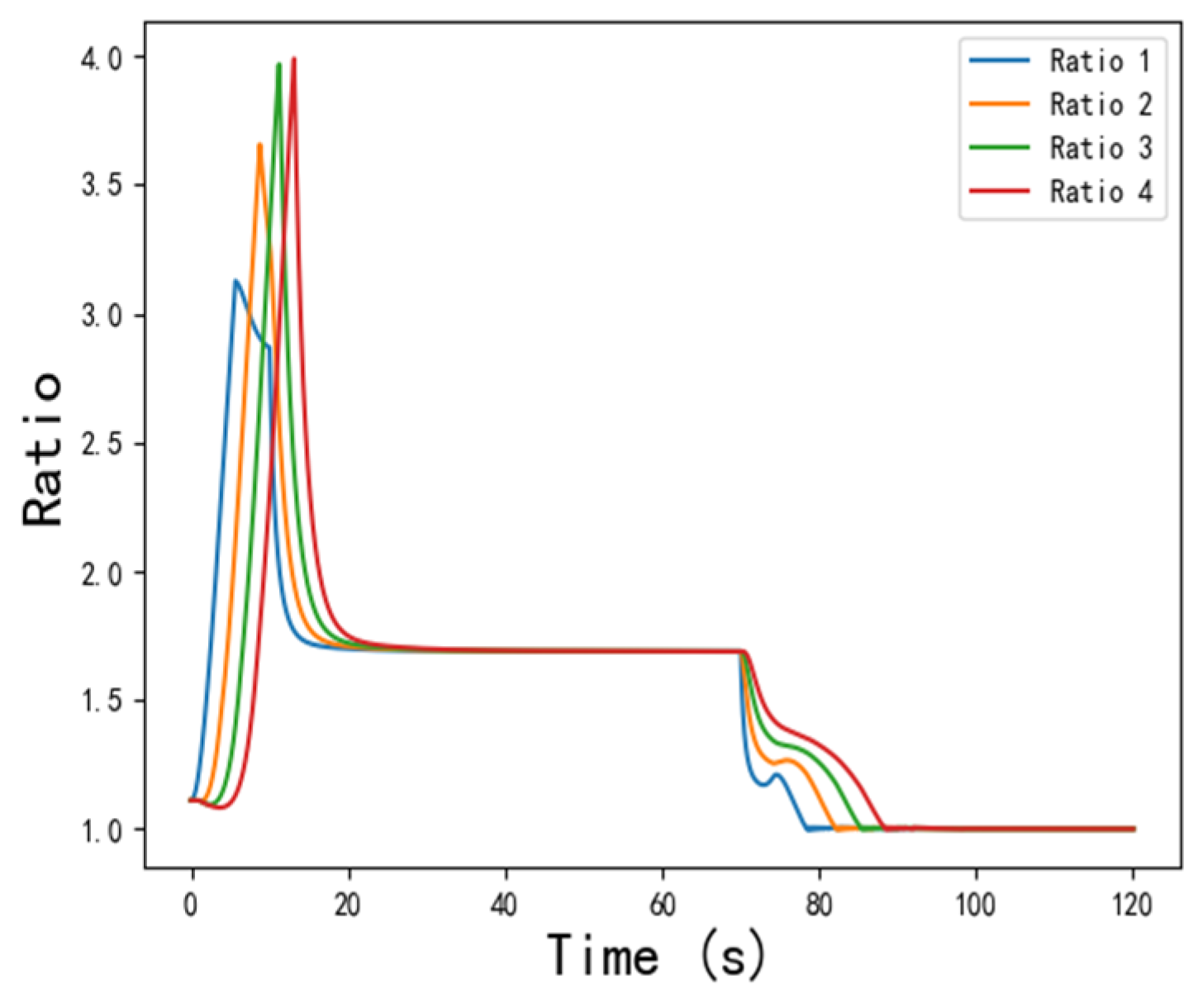
If the distance between adjacent cars in the motorcade exceeds the minimum safety distance, the following car can employ suitable control strategies to prevent a collision with the leading car. However, if the distance between adjacent cars in the motorcade falls below the minimum safety distance, there is a risk of collision between adjacent cars. The safety of the following model can be evaluated by calculating the ratio between the distance and the minimal safety distance. This ratio is depicted in Figure 9. Figure 9 illustrates the ratio n which represents the quotient of and .
Figure 9 clearly demonstrates that the ratio of the distance between automobiles and the required safety distance is consistently greater than 1 during motorcade driving. This indicates that the distance between adjacent cars is always greater than the minimum necessary safety distance. The control strategy of the car-following model ensures the security of the car-following process.
5. Conclusions
This research presents a novel safety distance model that takes into account the real-time variation of the adhesion coefficient during the braking process. The study examines the disparity between traditional and proposed safety distances for various combinations of initial adhesion coefficient and speed. It analyzes five scenarios and simulates a car-braking situation where the adhesion coefficient varies. The results indicate that the accuracy of the calculated safety distance is enhanced by a minimum of 14.99%.
A simulation is conducted to replicate the sequential actions of the motorcade, which involves the initial acceleration, maintaining a steady velocity, and subsequent deceleration. The simulation findings indicate that the stability of the system is influenced by the adjustment factor . When the value of is small, the control strategy exhibits low sensitivity towards speed errors and the distance between adjacent automobiles, resulting in a weak ability to achieve a stable state for the system. When the value of α is set to 2.5, the system achieves stability more quickly and exhibits reduced average errors in both speed and distance. Consequently, the system demonstrates improved stability. The simulation results show that the control strategy system effectively achieves stability within 32.11 s after the first car reaches a stable state. Furthermore, the control strategy guarantees the safety of the following processes even when the first car undergoes emergency braking at the maximum deceleration. In the future, we will explore the possibility of determining the safe distance for multiple cars in following scenarios.
Supplementary Materials
The following supporting information can be downloaded at: https://www.mdpi.com/article/10.3390/electronics13020421/s1, Table S1: Safety distance calculated in scene 1.
Author Contributions
Conceptualization, R.F.; methodology, M.M.; validation, A.L. and Y.Q.; writing—original draft preparation, M.M.; writing—review and editing, X.H.; visualization, L.Y. All authors have read and agreed to the published version of the manuscript.
Funding
This research was funded by General Project of National Natural Science Foundation of China under Grant 62120106011, the National Natural Science Foundation of China under Grant 62272384, Special Project for Local Services by the Shaanxi Provincial Department of Education in 2021 under Grant 21JC026, and the 29th School-Enterprise Cooperation Funding 2024.
Data Availability Statement
Data are contained within the article or Supplementary Material.
Acknowledgments
The authors thank Zhiming Chen and XINGYITONG Aerospace Technology (Nanjing) Co. for their support and contributions to this paper.
Conflicts of Interest
The authors declare no conflicts of interest.
References
- Jafaripournimchahi, A.; Hu, W.; Sun, L. Nonlinear stability analysis for an anticipation-memory car following model in the era of autonomous and connected vehicles. In Proceedings of the 2020 International Conference on Urban Engineering and Management Science (ICUEMS), Zhuhai, China, 24–26 April 2020; pp. 409–413. [Google Scholar]
- Zeng, Y.; Zhang, N. Review and new insights of the traffic flow lattice model for road vehicle traffic flow. In Proceedings of the 2014 IEEE International Conference on Control Science and Systems Engineering, Yantai, China, 29–30 December 2014; pp. 100–103. [Google Scholar]
- Yu, Y.; He, Z.; Qu, X. On the Impact of Prior Experiences in Car-Following Models: Model Development, Computational Efficiency, Comparative Analyses, and Extensive Applications. IEEE Trans. Cybern. 2023, 53, 1405–1418. [Google Scholar] [CrossRef] [PubMed]
- Abdelhalim, A.; Abbas, M. A Real-Time Safety-Based Optimal Velocity Model. IEEE Open J. Intell. Transp. Syst. 2022, 3, 165–175. [Google Scholar] [CrossRef]
- Xing, H.; Zhang, L.; Liu, Y. Effect of altruistic scenarios for individual car-following behavior. J. Tsinghua Univ. (Sci. Technol.) 2018, 58, 1000–1005. [Google Scholar]
- Li, X.; Luo, X.; He, M.; Chen, S. An improved car-following model considering the influence of space gap to the response. Phys. A Stat. Mech. Its Appl. 2018, 509, 536–545. [Google Scholar] [CrossRef]
- Wang, Y.; Zhang, J.; Lu, G. Influence of Driving Behaviors on the Stability in Car Following. IEEE Trans. Intell. Transp. Syst. 2018, 20, 1081–1098. [Google Scholar] [CrossRef]
- Kometani, E.; Sasaki, T. Dynamic Behavior of Traffic with a Nonlinear Spacing-speed Relationship. In Proceedings of the Symposium on Theory of Traffic Flow; Elsevier: New York, NY, USA, 1959; pp. 105–119. [Google Scholar]
- Park, M.; Kim, Y.; Yeo, H. Development of an Asymmetric Car-Following Model and Simulation Validation. IEEE Trans. Intell. Transp. Syst. 2020, 21, 3513–3524. [Google Scholar] [CrossRef]
- Gipps, P.G. A behavioural car-following model for computer simulation. Transp. Res. B Methodol. 1981, 15, 105–111. [Google Scholar] [CrossRef]
- Chen, Y.-L.; Wang, S.-C.; Wang, C.-A. Study on vehicle safety distance warning system. In Proceedings of the 2008 IEEE International Conference on Industrial Technology, Chengdu, China, 21–24 April 2008; pp. 1–6. [Google Scholar]
- Feng, G.; Wang, W.; Feng, J.; Tan, H.; Li, F. Modelling and Simulation for Safe Following Distance Based on Vehicle Braking Process. In Proceedings of the 2010 IEEE 7th International Conference on E-Business Engineering, Shanghai, China, 10–12 November 2010; pp. 385–388. [Google Scholar]
- Luo, Q.; Xun, L.; Cao, Z.; Huang, Y. Simulation analysis and study on car-following safety distance model based on braking process of leading vehicle. In Proceedings of the 2011 9th World Congress on Intelligent Control and Automation, Taipei, Taiwan, 21–25 June 2011; pp. 740–743. [Google Scholar]
- Duan, S.; Zhao, J. A model based on hierarchical safety distance algorithm for ACC control mode switching strategy. In Proceedings of the 2017 2nd International Conference on Image, Vision and Computing (ICIVC), Chengdu, China, 2–4 June 2017; pp. 904–908. [Google Scholar]
- Xia, F.; Li, S.; Li, H. Autonomous Obstacle Avoidance Control Strategy for Intelligent Vehicle Based on Lateral and Longitudinal Safety Distance Model. In Proceedings of the 2021 IEEE International Conference on Emergency Science and Information Technology (ICESIT), Chongqing, China, 22–24 November 2021; pp. 509–513. [Google Scholar]
- Lin, D.; Li, L. An Efficient Safety-Oriented Car-Following Model for Connected Automated Vehicles Considering Discrete Signals. IEEE Trans. Veh. Technol. 2023, 72, 9783–9795. [Google Scholar] [CrossRef]
- Erd, A.; Jaśkiewicz, M.; Koralewski, G.; Rutkowski, D.; Stokłosa, J. Experimental research of effectiveness of brakes in passenger cars under selected conditions. In Proceedings of the 2018 XI International Science-Technical Conference Automotive Safety, Častá, Slovakia, 18–20 April 2018; pp. 1–5. [Google Scholar]
- Lian, Y.; Zhao, Y.; Hu, L.; Tian, Y. Longitudinal Collision Avoidance Control of Electric Vehicles Based on a New Safety distance Model and Constrained-Regenerative-Braking-Strength-Continuity Braking Force Distribution Strategy. IEEE Trans. Veh. Technol. 2016, 65, 4079–4094. [Google Scholar] [CrossRef]
- Sevil, A.O.; Canevi, M.; Soylemez, M.T. Development of an Adaptive Autonomous Emergency Braking System Based on Road Friction. In Proceedings of the 2019 11th International Conference on Electrical and Electronics Engineering (ELECO), Bursa, Turkey, 28–30 November 2019; pp. 815–819. [Google Scholar]
- Guo, C.; Wang, X.; Su, L. Safety distance model for longitudinal collision avoidance of logistics vehicles considering slope and road adhesion coefficient. Proc. Inst. Mech. Eng. Part D J. Automob. Eng. 2021, 235, 498–512. [Google Scholar] [CrossRef]
- Castillo, J.J.; Cabrera, J.A.; Guerra, A.J.; Simón, A. A Novel Electrohydraulic Brake System with Tire–Road Friction Estimation and Continuous Brake Pressure Control. IEEE Trans. Ind. Electron. 2016, 63, 1863–1875. [Google Scholar] [CrossRef]
- Guan, R.; Fang, J.; Liu, J. Based on Binocular Identification Technology of Automobile Active Braking Safety Distance Model Research. In Proceedings of the 2016 International Symposium on Computer, Consumer and Control (IS3C), Xi’an, China, 4–6 July 2016; pp. 355–357. [Google Scholar]
- Cheng, J.; Du, F.; Qi, L.; Zhang, S.; Du, Q.; Ji, P. Research on Vehicle Cruise Control Strategy Based on Fixed Distance. In Proceedings of the 2022 International Conference on Mechanical and Electronics Engineering (ICMEE), Xi’an, China, 21–23 November 2022; pp. 122–126. [Google Scholar]
- Teng, C.; Ligang, G.; Zexu, W.; Qin, S.; Hao, N. Car Following Model Based on Driving Risk Field for Vehicle Infrastructure Cooperation. In Proceedings of the 2022 6th CAA International Conference on Vehicular Control and Intelligence (CVCI), Nanjing, China, 28–30 October 2022; pp. 1–6. [Google Scholar]
- Chen, C.-H. A Cell Probe-Based Method for Vehicle Speed Estimation. IEICE Trans. Fundam. Electron. Commun. Comput. Sci. 2020, 103, 265–267. [Google Scholar] [CrossRef]
- Surya, H.R.; Raju, N.; Arkatkar, S.S. Stability Analysis of Mixed Traffic Flow using Car-Following Models on Trajectory Data. In Proceedings of the 2021 International Conference on COMmunication Systems & NETworkS (COMSNETS), Bangalore, India, 5–9 January 2021; pp. 656–661. [Google Scholar]
- Jin, H.; Hao, H.; Yang, X. Continuous and Discrete Analysis of Local Stability for Car-Following Model with Speed-Based Desired-Headway. IEEE Trans. Intell. Transp. Syst. 2021, 23, 5374–5386. [Google Scholar] [CrossRef]
- Ngoduy, D. Analytical studies on the instabilities of heterogeneous intelligent traffic flow. Commun. Nonlinear Sci. Numer. Simul. 2013, 18, 2699–2706. [Google Scholar] [CrossRef]
- Wang, M.; Hoogendoorn, S.P.; Daamen, W.; van Arem, B.; Shyrokau, B.; Happee, R. Delay-compensating strategy to enhance string stability of adaptive cruise controlled car followings. Transp. B Transp. Dyn. 2018, 6, 211–229. [Google Scholar]
- Li, Y.; Tang, C.; Peeta, S.; Wang, Y. Nonlinear Consensus-Based Connected Vehicle Platoon Control Incorporating Car-Following Interactions and Heterogeneous Time Delays. IEEE Trans. Intell. Transp. Syst. 2019, 20, 2209–2219. [Google Scholar] [CrossRef]
- Jia, B.; Yang, D.; Zhang, X.; Wu, Y.; Guo, Q. Car-following model considering the lane-changing prevention effect and its stability analysis. Eur. Phys. J. B 2020, 93, 153. [Google Scholar] [CrossRef]
- Wan, N.; Zhang, C.; Vahidi, A. Probabilistic Anticipation and Control in Autonomous Car Following. IEEE Trans. Control. Syst. Technol. 2019, 27, 30–38. [Google Scholar] [CrossRef]
- Chen, Y.-J.; Li, X.-G.; Zhang, Y.; Niculescu, S.-I.; Çela, A. Stability Analysis of Car-Following Systems with Uniformly Distributed Delays Using Frequency-Sweeping Approach. IEEE Access 2021, 9, 69747–69755. [Google Scholar] [CrossRef]
Figure 1.
The process of braking at maximum deceleration.

Figure 2.
TSD calculated in scene 1.

Figure 3.
PSD calculated in scene 1.
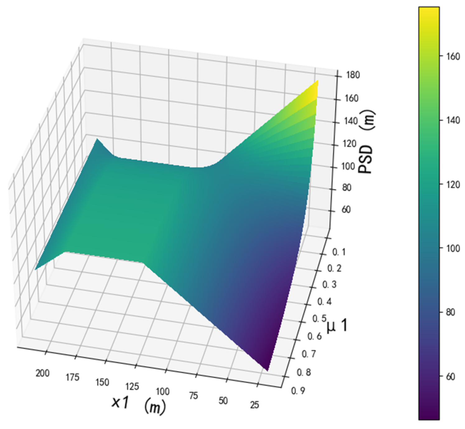
Figure 4.
The difference between TSD and PSD calculated in scene 1.
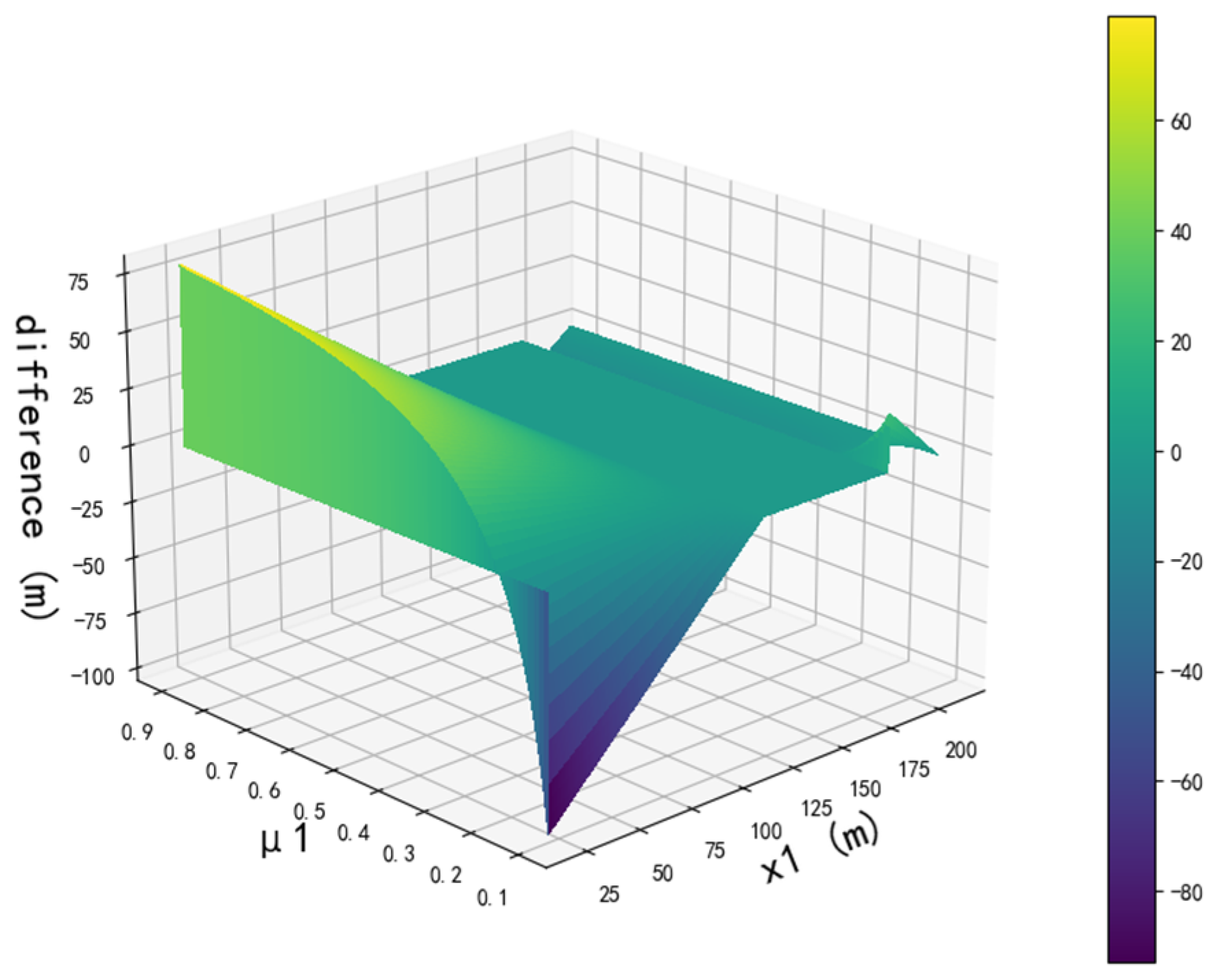
Figure 5.
The reaction braking process of the following car with .

Figure 6.
The reaction braking process of the following car with .
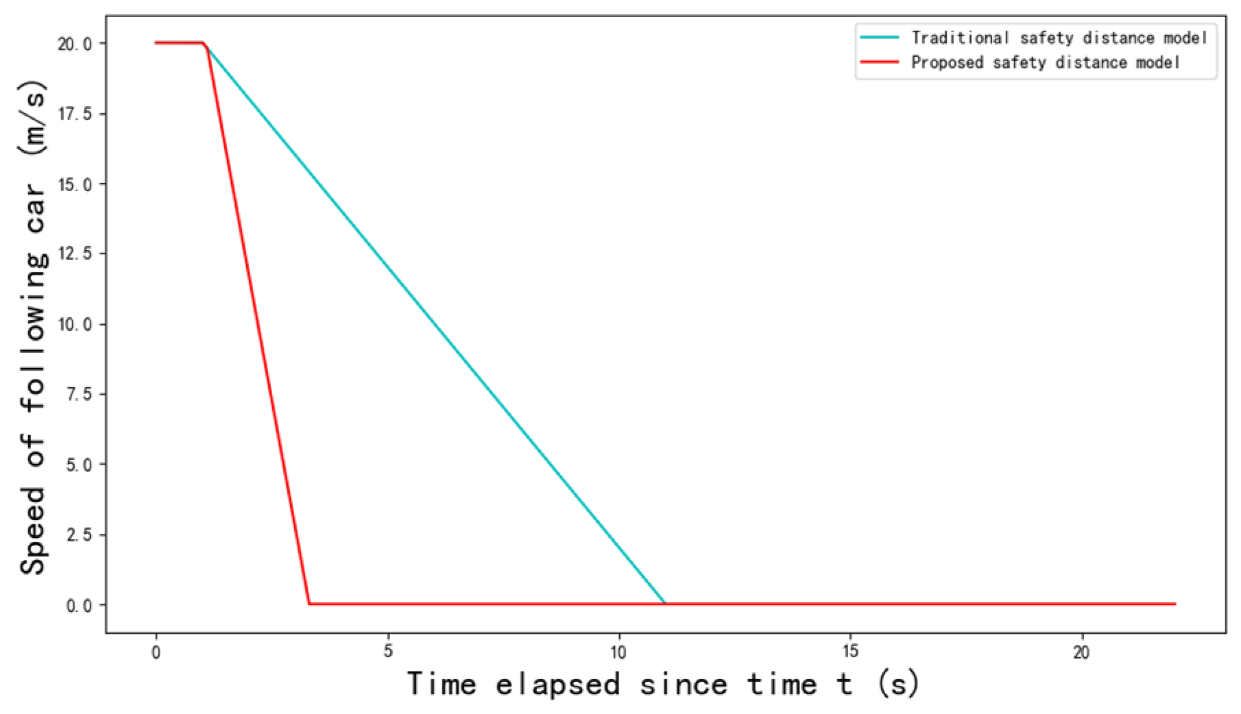
Figure 7.
Speed curve of car-following process.
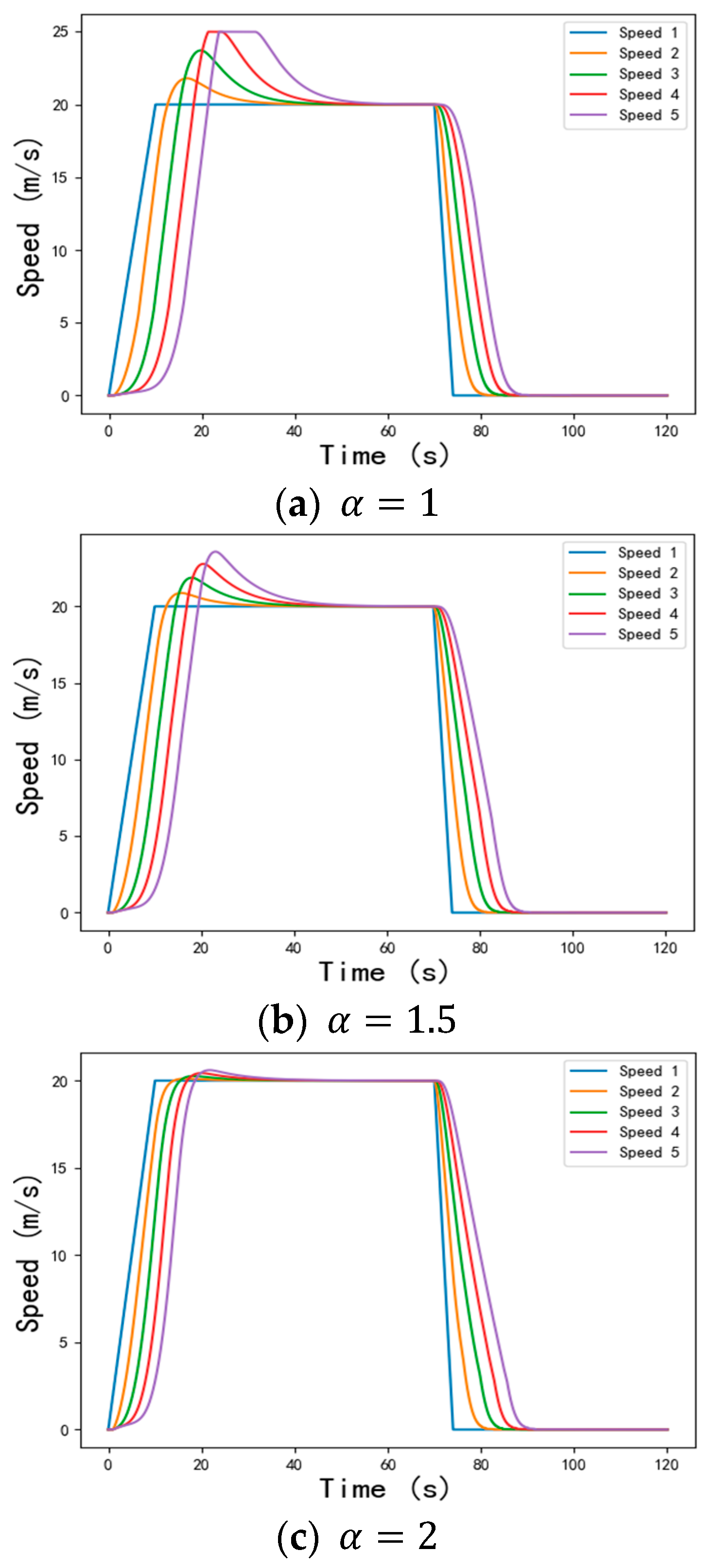

Figure 8.
The distance between adjacent cars.
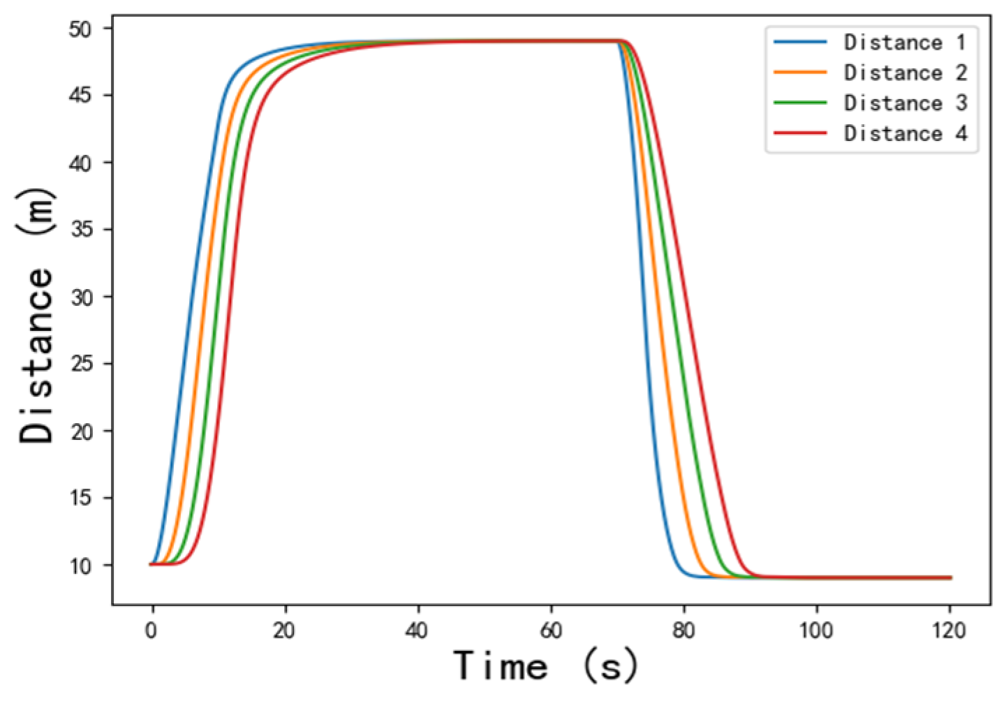
Figure 9.
The ratio of the distance and the minimum safety distance.

Table 1.
Relevant parameters.
| Symbol | Parameter Description |
|---|---|
| Position of the car numbered n at time t | |
| Speed of the car numbered n at time t | |
| Acceleration of the car numbered n at time t | |
| Driver’s reaction time | |
| Maximum deceleration of the car numbered n at time t | |
| Maximum comfortable acceleration of the car numbered n | |
| Maximum allowable driving speed on the road | |
| Adhesion coefficient at position x | |
| The acceleration of gravity | |
| Length of the car numbered n |
Table 2.
Parameter settings of scenes.
| Scene No. | (m/s) | (m/s) | (m) | |
|---|---|---|---|---|
| Scene 1 | 10 | 20 | 0.2 | 185 |
| Scene 2 | 10 | 20 | 0.8 | 185 |
| Scene 3 | 10 | 10 | 0.2 | 40 |
| Scene 4 | 10 | 10 | 0.8 | 20 |
| Scene 5 | 20 | 20 | 0.2 | 110 |
| Scene 6 | 20 | 20 | 0.8 | 40 |
Table 3.
Some combinations of and .
| Combination Number | (m) | |
|---|---|---|
| Combination 1 | 0.9 | 20.2 |
| Combination 2 | 0.9 | 119.8 |
| Combination 3 | 0.1 | 20.2 |
| Combination 4 | 0.1 | 119.8 |
Table 4.
Comparison of stability when takes different values.
| Time to Steady State (s) | Speed Error (m/s) | Distance Error (m/s2) | |
|---|---|---|---|
| 1 | 62.29 | 0.0176 | 0.0882 |
| 1.5 | 56.90 | 0.0073 | 0.0365 |
| 2 | 43.76 | 0.0013 | 0.0067 |
| 2.5 | 42.11 | 0.0009 | 0.0039 |
| 3 | 47.92 | 0.0023 | 0.0107 |
Disclaimer/Publisher’s Note: The statements, opinions and data contained in all publications are solely those of the individual author(s) and contributor(s) and not of MDPI and/or the editor(s). MDPI and/or the editor(s) disclaim responsibility for any injury to people or property resulting from any ideas, methods, instructions or products referred to in the content. |
© 2024 by the authors. Licensee MDPI, Basel, Switzerland. This article is an open access article distributed under the terms and conditions of the Creative Commons Attribution (CC BY) license (https://creativecommons.org/licenses/by/4.0/).
Share and Cite
MDPI and ACS Style
Fei, R.; Ma, M.; Hei, X.; Yang, L.; Li, A.; Qiu, Y. A New Safety Distance Model Based on Braking Process Considering Adhesion Coefficient. Electronics 2024, 13, 421. https://doi.org/10.3390/electronics13020421
AMA Style
Fei R, Ma M, Hei X, Yang L, Li A, Qiu Y. A New Safety Distance Model Based on Braking Process Considering Adhesion Coefficient. Electronics. 2024; 13(2):421. https://doi.org/10.3390/electronics13020421
Chicago/Turabian StyleFei, Rong, Mengyang Ma, Xinhong Hei, Lu Yang, Aimin Li, and Yuan Qiu. 2024. "A New Safety Distance Model Based on Braking Process Considering Adhesion Coefficient" Electronics 13, no. 2: 421. https://doi.org/10.3390/electronics13020421
Note that from the first issue of 2016, this journal uses article numbers instead of page numbers. See further details here.