

Tensorized Discrete Multi-View Spectral Clustering


Abstract
1. Introduction
- Our model makes spectral clustering collaborate with spectral rotation in a unified framework for multi-view clustering. Thus, it directly obtains a discrete label matrix without post-processing.
- Our method effectively encodes both the complementary information and discriminative information of indicator matrices of the views by using a weighted tensor nuclear norm regularizer.
- Our weighted scheme directly considers the relationship between views for clustering. Thus, the learned indicator matrix effectively encodes discriminative information. Extensive experimental results indicate the effectiveness and efficiency of our proposed algorithm.
2. Related Works
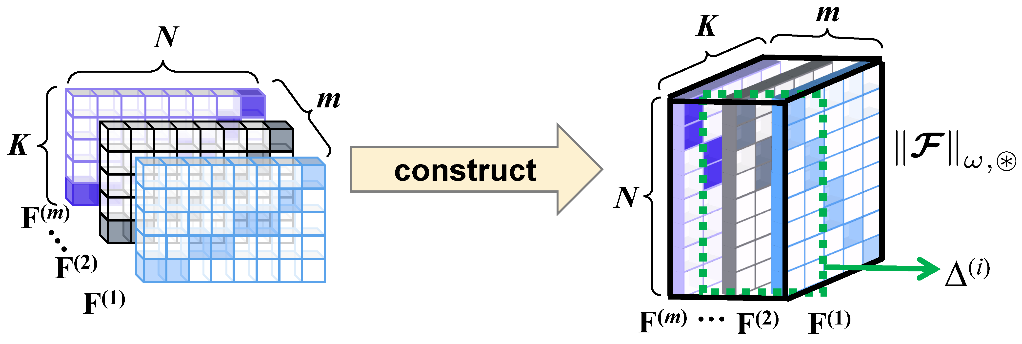
3. Notations
4. Proposed Method
4.1. Problem Formulation and Objective Function
4.2. Optimization
- Solving with fixed and . In this case, each can be solved independently. Thus, for the v-th rotation matrix , Equation (7) becomes
- Solving with fixed . Thus, Equation (7) becomes
| Algorithm 1 Solve |
Input: The matrix , , , , and . Output: , .
|
- Solving with other fixed variables. Now, can be optimized by sub-problem (21):
- Solving and . can be updated by . can be updated by , where is a positive number larger than 1.
- Solving with fixed , and . In this case, the problem (7) becomes
| Algorithm 2 Solving |
Input:. Output: .
|
- Solving . For the sake of a convincing description, let which is known. In this case, can be solved by
- Solving . According to [8], the optimal is
| Algorithm 3 Tensorized discrete multi-view spectral clustering |
Input:Data matrices , hyperparameters: K, , and . Output: The label of data.
|
4.3. Complexity Analysis
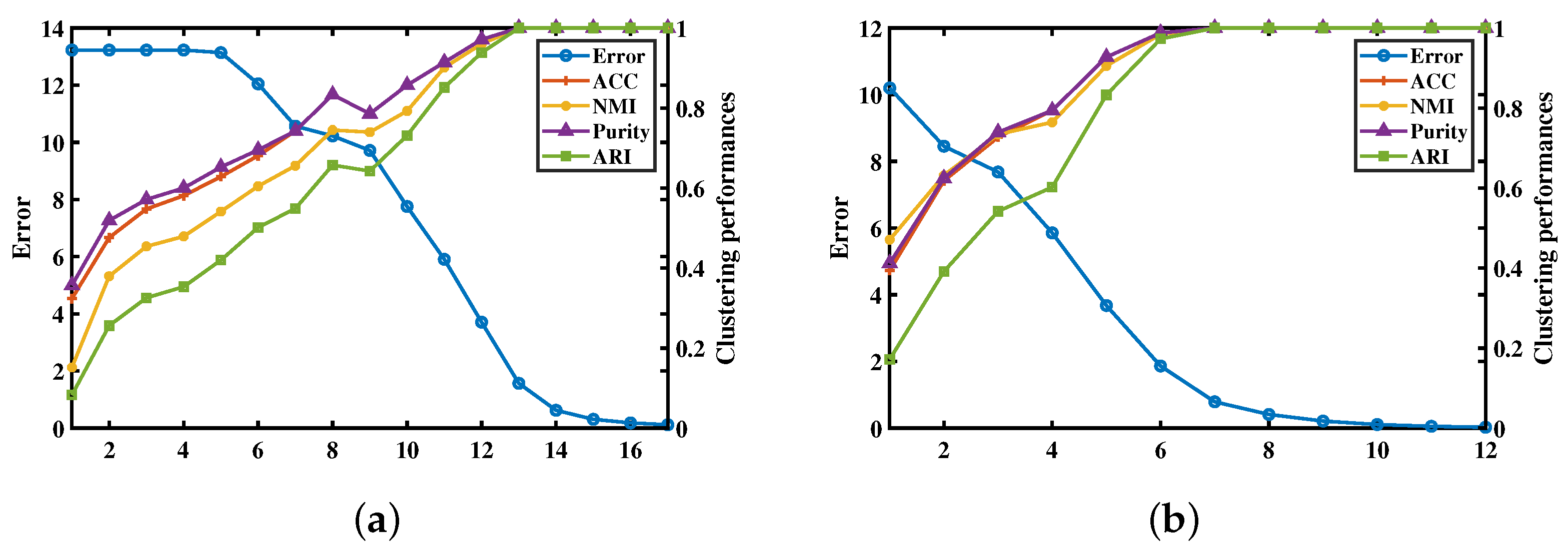
5. Converge Analysis
6. Experiment
6.1. Experimental Setup
6.1.1. Datasets
- Caltech101 (Cal-101) (https://tensorflow.google.cn/datasets/catalog/caltech101 (accessed on 10 September 2023)) [46] dataset has 101 classes. Like [9], we chose 441 samples with seven categories in our experiments. These samples have three views, i.e., 2560-dimensional (D) SIFT feature, 1160-D LBP features and 620-D HOG feature.
- The MSRC-v1 (https://mldta.com/dataset/msrc-v1/ (accessed on 10 September 2023)) [47] dataset includes eight categories. Like [9], we chose 210 samples with seven categories in our experiments. These samples have five views, i.e., 24-D color moment, 512-D GIST feature, 576-D Histogram of Oriented Gradient, 254-D CENTRIST feature and 256-D LBP feature.
- The Yale (http://vision.ucsd.edu/content/yale-face-database (accessed on 10 September 2023)) dataset has 165 samples with 15 people. These samples have different conditions, such as occlusion changes, facial expression and with or without glasses. In the experiment, it has three different views, i.e., 3304-D LBP feature, 6750-D Gabor feature and 4096-D intensity feature.
- The ORL (http://www.uk.research.att.com/facedatabase.html (accessed on 10 September 2023)) dataset consists of 400 samples with 40 different people. These samples have different conditions, such as facial expression and occlusion changes. In the experiment, we use three views, i.e., 6750-D Gabor feature, 4096-D intensity feature, and 3340-D LBP feature.
- Scene-15 (https://www.kaggle.com/datasets/zaiyankhan/15scene-dataset (accessed on 10 September 2023)) [48] is a scene dataset with 15 different natural scenes. It contains 4485 samples with three different views, i.e., 1800-D PHOW featue, 1240-D CENTRIST feature and 1180-D PRI-CoLBP feature.
- The ESP-GAME (https://www.kaggle.com/datasets/parhamsalar/espgame (accessed on 10 September 2023)) dataset contains 11,032 samples over seven categories. It has two different views, each of them is 100 dimensions.
6.1.2. Comparisons
6.2. Experimental Results and Analysis
6.2.1. Performance Comparison
- Multi-view clustering methods are overall superior to SC with the best performance. The reason may be that, compared with single-view representation, multi-view representation can provide some useful complementary information, and these multi-view methods make good use of these complementary information. In the Scene-15 database, except for CSMSC, non-tensor multi-view clustering methods are overall inferior to SC. The reason may be that there is a large difference between the views for clustering, and in these methods, weights for different views are independent and neglect the relationship between views for clustering. It also indicates that it is very important to design a suitable weighted scheme for improving multi-view clustering.
- Among the non-tensor clustering methods, the adaptive weighted multi-view spectral clustering method AMGL and coregularized spectral clustering Co-reg are overall inferior to the other methods. The reason may be that the performance results of AMGL and Co-reg heavily depend on the predefined graph, and it is difficult to manually select a suitable graph in real applications due to the complex distribution of data.
- Tensor-based clustering methods, such as t-SVD-MSC, ETLMSC, LTCSPC and our proposed method, are superior to the other methods. This is probably because tensor-based clustering methods effectively exploit the complementary information and spatial structure embedded in the graphs or affinity matrices of different views. It also indicates that the difference between graphs or affinity matrices of different view helps provide useful complementary information for clustering.
- Our proposed method is superior to the other clustering methods. This is probably because our proposed method explicitly considers the effect of different views for clustering, and the assigned weights for different views are related. Moreover, our method directly obtains a discrete label matrix for data, while the other methods require extra post-processing, which results in a sub-optimal discrete solution. It is worth noting that after adjusting the parameters to achieve optimal results, we observed that the standard deviation of our algorithm across all datasets is 0. This indicates that our algorithm exhibits excellent robustness.
- LTCSPC utilizes weighted tensor nuclear norm regularization to minimize the discrepancy between the view indicator matrices, making full use of the complementary information hidden in the views. Therefore, its clustering performance is better than the adaptive weighted multi-view spectral clustering method (AMGL) and the adaptive graph learning clustering method (MVGL). But LTCSPC is inferior to our proposed method. It indicates that spectral rotation helps further improve the clustering performance results and is a reasonable scheme to obtain a discrete solution for spectral clustering.
- Our model achieved relatively good clustering accuracy on various types of multi-view datasets, including Caltech101, MSRC-v1, Yale, ORL, Scene-15, and ESP-GAME. This consistent high performance demonstrates the strong generalization ability of our model, enabling it to adapt to the characteristics of different datasets and produce robust clustering results.
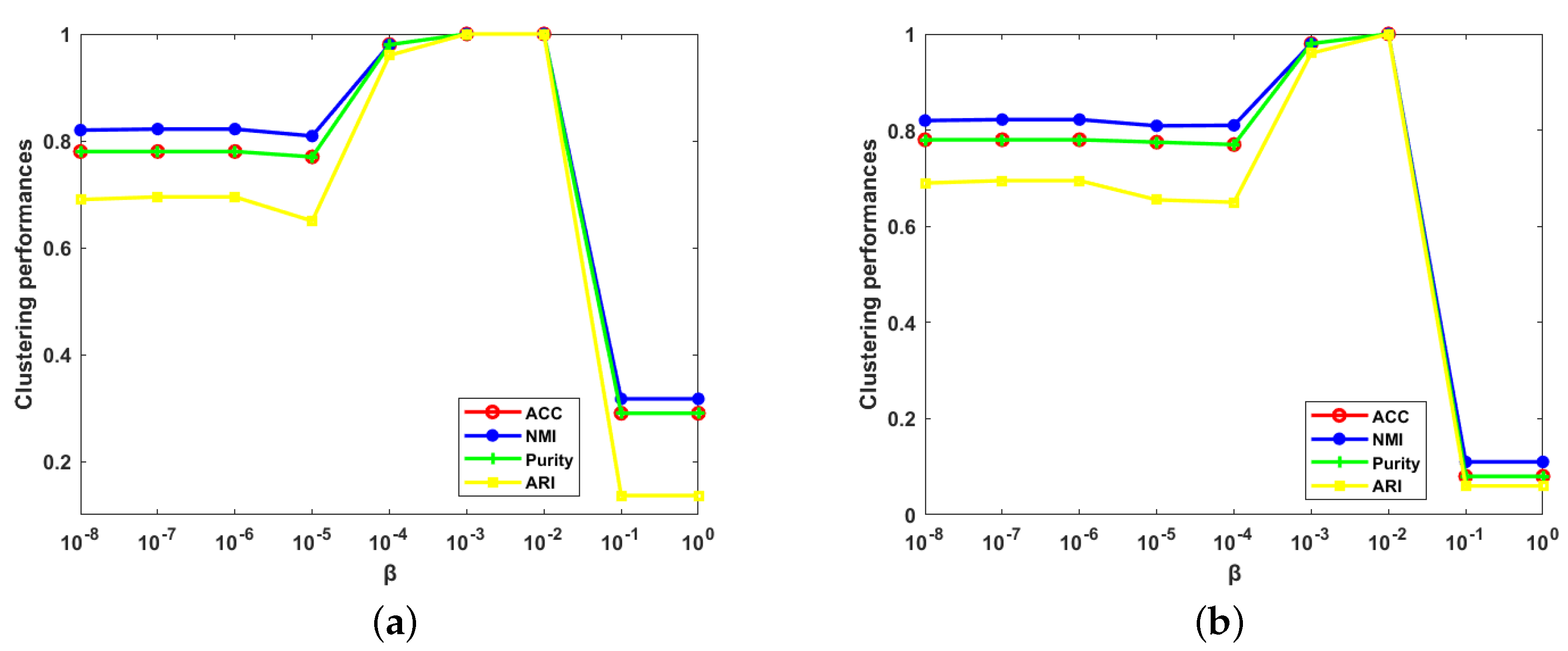
6.2.2. Parameter Analysis
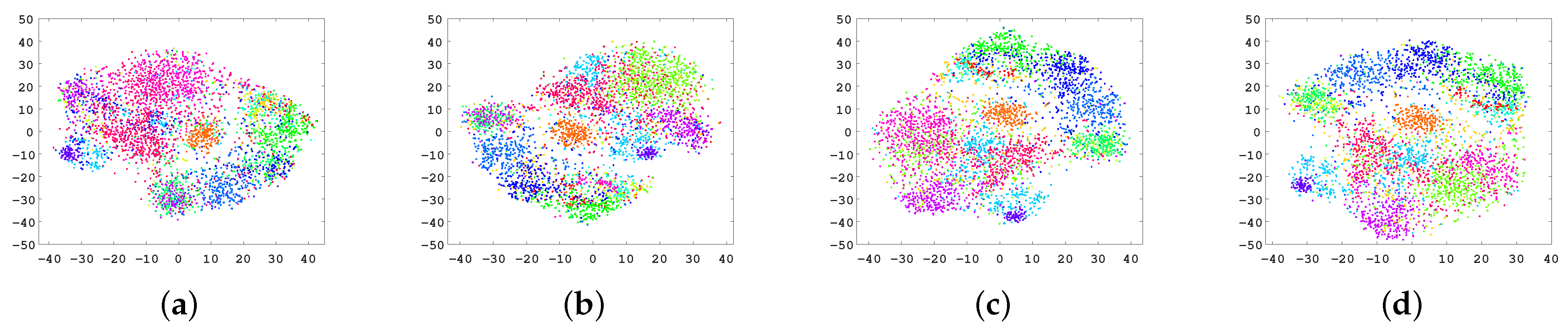
6.2.3. Ablation and Visualization
7. Conclusions
Author Contributions
Funding
Data Availability Statement
Conflicts of Interest
References
- Xie, Y.; Tao, D.; Zhang, W.; Yan, L.; Lei, Z.; Qu, Y. On Unifying Multi-view Self-Representations for Clustering by Tensor Multi-rank Minimization. Proc. IJCV 2018, 126, 1157–1179. [Google Scholar] [CrossRef]
- Xie, D.; Zhang, X.; Gao, Q.; Han, J.; Xiao, S.; Gao, X. Multiview Clustering by Joint Latent Representation and Similarity Learning. IEEE Trans. Cybern. 2020, 50, 4848–4854. [Google Scholar] [CrossRef]
- Liu, X.; Zhu, X.; Li, M.; Wang, L.; Tang, C.; Yin, J.; Shen, D.; Wang, H.; Gao, W. Late Fusion Incomplete Multi-View Clustering. IEEE Trans. Pattern Anal. Mach. Intell. 2018, 41, 2410–2423. [Google Scholar] [CrossRef]
- Hu, P.; Peng, X.; Zhu, H.; Zhen, L.; Lin, J.; Yan, H.; Peng, D. Deep Semisupervised Multiview Learning with Increasing Views. IEEE Trans. Cybern. 2021, 52, 12954–12965. [Google Scholar] [CrossRef]
- Wang, Q.; Lian, H.; Sun, G.; Gao, Q.; Jiao, L. iCmSC: Incomplete Cross-Modal Subspace Clustering. IEEE Trans. Image Process. 2021, 30, 305–317. [Google Scholar] [CrossRef]
- Lu, H.; Xu, H.; Wang, Q.; Gao, Q.; Yang, M.; Gao, X. Efficient Multi-View -Means for Image Clustering. IEEE Trans. Image Process. 2024, 33, 273–284. [Google Scholar] [CrossRef]
- Kumar, A.; Rai, P. Co-regularized multi-view spectral clustering. In Proceedings of the 24th International Conference on Neural Information Processing Systems (NIPS’11), Granada, Spain, 12–15 December 2011; Curran Associates Inc.: Red Hook, NY, USA, 2011; Volume 24, pp. 1413–1421. [Google Scholar]
- Nie, F.; Li, J.; Li, X. Parameter-Free Auto-Weighted Multiple Graph Learning: A Framework for Multiview Clustering and Semi-Supervised Classification. In Proceedings of the Twenty-Fifth International Joint Conference on Artificial Intelligence (IJCAI-16), New York, NY, USA, 9–15 July 2016; pp. 1881–1887. [Google Scholar]
- Xu, H.; Zhang, X.; Xia, W.; Gao, Q.; Gao, X. Low-rank tensor constrained co-regularized multi-view spectral clustering. Neural Netw. 2020, 132, 245–252. [Google Scholar] [CrossRef]
- Zhan, K.; Zhang, C.; Guan, J.; Wang, J. Graph Learning for Multiview Clustering. IEEE Trans. Cybern. 2018, 48, 2887–2895. [Google Scholar] [CrossRef]
- Yun, Y.; Li, J.; Gao, Q.; Yang, M.; Gao, X. Low-rank discrete multi-view spectral clustering. Neural Netw. 2023, 166, 137–147. [Google Scholar] [CrossRef]
- Liu, X.; Zhu, X.; Li, M.; Tang, C.; Gao, W. Efficient and Effective Incomplete Multi-View Clustering. In Proceedings of the AAAI Conference on Artificial Intelligence, Honolulu, HI, USA, 27 January–1 February 2019; Volume 33, pp. 4392–4399. [Google Scholar]
- Jiang, T.; Gao, Q. Fast multiple graphs learning for multi-view clustering. Neural Netw. 2022, 155, 348–359. [Google Scholar] [CrossRef]
- Nie, F.; Cai, G.; Li, X. Multi-View Clustering and Semi-Supervised Classification with Adaptive Neighbours. In Proceedings of the AAAI Conference on Artificial Intelligence, San Francisco, CA, USA, 4–9 February 2017; pp. 2408–2414. [Google Scholar]
- Nie, F.; Li, J.; Li, X. Self-weighted Multiview Clustering with Multiple Graphs. In Proceedings of the International Joint Conference on Artificial Intelligence, Melbourne, Australia, 19–25 August 2017; pp. 2564–2570. [Google Scholar]
- Yu, S.X.; Shi, J. Multiclass Spectral Clustering. In Proceedings of the Ninth IEEE International Conference on Computer Vision, Nice, France, 13–16 October 2003; Volume 1, pp. 313–319. [Google Scholar]
- Pang, Y.; Xie, J.; Nie, F.; Li, X. Spectral Clustering by Joint Spectral Embedding and Spectral Rotation. IEEE Trans. Cybern 2020, 50, 247–258. [Google Scholar] [CrossRef]
- Wang, Z.; Li, Z.; Wang, R.; Nie, F.; Li, X. Large Graph Clustering with Simultaneous Spectral Embedding and Discretization. IEEE Trans. Pattern Anal. Mach. Intell. 2020, 43, 4426–4440. [Google Scholar] [CrossRef]
- Yang, Y.; Shen, F.; Huang, Z.; Shen, H.T. A Unified Framework for Discrete Spectral Clustering. In Proceedings of the International Joint Conference on Artificial Intelligence, New York, NY, USA, 9–15 July 2016; pp. 2273–2279. [Google Scholar]
- Zhong, G.; Pun, C. A Unified Framework for Multi-view Spectral Clustering. In Proceedings of the IEEE International Conference on Data Engineering (ICDE), Dallas, TX, USA, 20–24 April 2020; pp. 1854–1857. [Google Scholar]
- Wan, Z.; Xu, H.; Gao, Q. Multi-view clustering by joint spectral embedding and spectral rotation. Neurocomputing 2021, 462, 123–131. [Google Scholar] [CrossRef]
- Shi, S.; Nie, F.; Wang, R.; Li, X. Auto-weighted multi-view clustering via spectral embedding. Neurocomputing 2020, 399, 369–379. [Google Scholar] [CrossRef]
- Gao, Q.; Zhang, P.; Xia, W.; Xie, D.; Gao, X.; Tao, D. Enhanced Tensor RPCA and its Application. IEEE Trans. Pattern Anal. Mach. Intell. 2021, 43, 2133–2140. [Google Scholar] [CrossRef]
- Xia, W.; Zhang, X.; Gao, Q.; Shu, X.; Han, J.; Gao, X. Multi-view Subspace Clustering by an Enhanced Tensor Nuclear Norm. IEEE Trans. Cybern. 2021, 52, 8962–8975. [Google Scholar] [CrossRef]
- Xie, Y.; Zhang, W.; Qu, Y.; Dai, L.; Tao, D. Hyper-Laplacian Regularized Multilinear Multiview Self-Representations for Clustering and Semisupervised Learning. IEEE Trans. Cybern. 2020, 50, 572–586. [Google Scholar] [CrossRef]
- Wen, J.; Xu, Y.; Liu, H. Incomplete Multiview Spectral Clustering With Adaptive Graph Learning. IEEE Trans. Cybern. 2020, 50, 1418–1429. [Google Scholar] [CrossRef]
- Wen, J.; Zhang, Z.; Zhang, Z.; Fei, L.; Wang, M. Generalized Incomplete Multiview Clustering with Flexible Locality Structure Diffusion. IEEE Trans. Cybern. 2020, 51, 101–114. [Google Scholar] [CrossRef]
- Zong, L.; Zhang, X.; Liu, X.; Yu, H. Weighted Multi-view Spectral Clustering based on Spectral Perturbation. In Proceedings of the AAAI Conference on Artificial Intelligence, New Orleans, LA, USA, 2–7 February 2018; pp. 4621–4628. [Google Scholar]
- Li, Z.; Tang, C.; Liu, X.; Zheng, X.; Yue, G.; Zhang, W.; Zhu, E. Consensus Graph Learning for Multi-view Clustering. IEEE Trans. Multimed. 2021, 24, 2461–2472. [Google Scholar] [CrossRef]
- Tan, Y.; Liu, Y.; Huang, S.; Feng, W.; Lv, J. Sample-Level Multi-View Graph Clustering. In Proceedings of the IEEE/CVF Conference on Computer Vision and Pattern Recognition (CVPR), Vancouver, BC, Canada, 18–22 June 2023; pp. 23966–23975. [Google Scholar]
- Xia, R.; Pan, Y.; Du, L.; Yin, J. Robust multi-view spectral clustering via low-rank and sparse decomposition. In Proceedings of the AAAI Conference on Artificial Intelligence, Québec City, QC, Canada, 27–31 July 2014; pp. 2149–2155. [Google Scholar]
- Tang, C.; Zhu, X.; Liu, X.; Li, M.; Wang, P.; Zhang, C.; Wang, L. Learning a Joint Affinity Graph for Multiview Subspace Clustering. IEEE Trans. Multimed. 2019, 21, 1724–1736. [Google Scholar] [CrossRef]
- Tang, C.; Liu, X.; Zhu, X.; Zhu, E.; Gao, W. CGD: Multi-View Clustering via Cross-View Graph Diffusion. In Proceedings of the AAAI Conference on Artificial Intelligence, New York, NY, USA, 7–12 February 2020; Volume 34, pp. 5924–5931. [Google Scholar]
- Wu, J.; Lin, Z.; Zha, H. Essential Tensor Learning for Multi-view Spectral Clustering. IEEE Trans. Image Process. 2019, 28, 5910–5922. [Google Scholar] [CrossRef]
- Zhan, K.; Nie, F.; Wang, J.; Yang, Y. Multiview Consensus Graph Clustering. IEEE Trans. Image Process. 2019, 28, 1261–1270. [Google Scholar] [CrossRef]
- Ding, C.H.Q.; Li, T.; Jordan, M.I. Convex and Semi-Nonnegative Matrix Factorizations. IEEE Trans. Pattern Anal. Mach. Intell. 2010, 32, 45–55. [Google Scholar] [CrossRef]
- Shi, S.; Nie, F.; Wang, R.; Li, X. Multi-View Clustering via Nonnegative and Orthogonal Graph Reconstruction. IEEE Trans. Neural Netw. Learn. Syst. 2021, 34, 201–214. [Google Scholar] [CrossRef]
- Yang, H.; Gao, Q.; Xia, W.; Yang, M.; Gao, X. Multiview Spectral Clustering With Bipartite Graph. IEEE Trans. Image Process. 2022, 31, 3591–3605. [Google Scholar] [CrossRef]
- Nie, F.; Tian, L.; Li, X. Multiview Clustering via Adaptively Weighted Procrustes. In Proceedings of the 24th ACM SIGKDD International Conference on Knowledge Discovery & Data Mining, KDD 2018, London, UK, 19–23 August 2018; Guo, Y., Farooq, F., Eds.; ACM: New York, NY, USA, 2018; pp. 2022–2030. [Google Scholar]
- Han, Y.; Zhu, L.; Cheng, Z.; Li, J.; Liu, X. Discrete Optimal Graph Clustering. IEEE Trans. Cybern. 2020, 50, 1697–1710. [Google Scholar] [CrossRef]
- Xia, W.; Gao, Q.; Wang, Q.; Gao, X.; Ding, C.; Tao, D. Tensorized Bipartite Graph Learning for Multi-View Clustering. IEEE Trans. Pattern Anal. Mach. Intell. 2023, 45, 5187–5202. [Google Scholar] [CrossRef]
- Kilmer, M.E.; Martin, C.D. Factorization strategies for third-order tensors. Linear Algebra Its Appl. 2011, 435, 641–658. [Google Scholar] [CrossRef]
- Lin, Z.; Chen, M.; Ma, Y. The augmented lagrange multiplier method for exact recovery of corrupted low-rank matrices. arXiv 2010, arXiv:1009.5055. [Google Scholar]
- Gao, Q.; Xu, S.; Chen, F.; Ding, C.; Gao, X.; Li, Y. R1-2-DPCA and Face Recognition. IEEE Trans. Cybern. 2019, 49, 1212–1223. [Google Scholar] [CrossRef] [PubMed]
- Lin, T.; Ma, S.; Zhang, S. Iteration complexity analysis of multi-block ADMM for a family of convex minimization without strong convexity. J. Sci. Comput. 2016, 69, 52–81. [Google Scholar] [CrossRef]
- Fei-Fei, L.; Fergus, R.; Perona, P. Learning generative visual models from few training examples: An incremental bayesian approach tested on 101 object categories. Comput. Vis. Image Underst. 2007, 106, 59–70. [Google Scholar] [CrossRef]
- Winn, J.; Jojic, N. Locus: Learning object classes with unsupervised segmentation. In Proceedings of the Tenth IEEE International Conference on Computer Vision, Beijing, China, 17–21 October 2005; Volume 1, pp. 756–763. [Google Scholar]
- Oliva, A.; Torralba, A. Modeling the Shape of the Scene: A Holistic Representation of the Spatial Envelope. Int. J. Comput. Vis. 2001, 42, 145–175. [Google Scholar] [CrossRef]
- Ng, A.Y.; Jordan, M.I.; Weiss, Y. On spectral clustering: Analysis and an algorithm. In Proceedings of the 14th International Conference on Neural Information Processing Systems: Natural and Synthetic (NIPS’01), Vancouver, BC, Canada, 3–8 December 2001; Volume 14, pp. 849–856. [Google Scholar]
- Luo, S.; Zhang, C.; Zhang, W.; Cao, X. Consistent and Specific Multi-View Subspace Clustering. In Proceedings of the AAAI Conference on Artificial Intelligence, New Orleans, LA, USA, 2–7 February 2018; pp. 3730–3737. [Google Scholar]


| Dataset | Yale | MSRC | Cal101 | ORL | Scene-15 | ESP-IMG |
|---|---|---|---|---|---|---|
| k | 8 | 8 | 8 | 8 | 8 | 80 |
| 0.01 | 0.01 | 0.01 | 0.01 | 0.001 | 0.01 | |
| [1, 5, 0.1] | [1, 100, 10, 0.1, 5] | [5, 0.1, 1] | [1, 10, 100] | [1, 5, 100] | [10, 1] |
| Dataset | Cal-101 | MSRC-V1 | ||||||
| Metric | ACC | NMI | Purity | ARI | ACC | NMI | Purity | ARI |
| SC-best | 0.545 ± 0.03 | 0.431 ± 0.02 | 0.624 ± 0.02 | 0.390 ± 0.02 | 0.663 ± 0.04 | 0.534 ± 0.02 | 0.674 ± 0.03 | 0.441 ± 0.03 |
| AMGL | 0.481 ± 0.03 | 0.345 ± 0.02 | 0.540 ± 0.02 | 0.184 ± 0.03 | 0.732 ± 0.04 | 0.669 ± 0.02 | 0.740 ± 0.02 | 0.543 ± 0.02 |
| CSMSC | 0.567 ± 0.00 | 0.480 ± 0.00 | 0.633 ± 0.00 | 0.395 ± 0.00 | 0.742 ± 0.01 | 0.597 ± 0.01 | 0.742 ± 0.01 | 0.532 ± 0.01 |
| MLAN | 0.587 ± 0.00 | 0.462 ± 0.00 | 0.655 ± 0.00 | 0.347 ± 0.00 | 0.743 ± 0.00 | 0.746 ± 0.00 | 0.805 ± 0.00 | 0.661 ± 0.00 |
| Co-Reg | 0.452 ± 0.01 | 0.283 ± 0.01 | 0.502 ± 0.01 | 0.234 ± 0.01 | 0.744 ± 0.02 | 0.632 ± 0.01 | 0.750 ± 0.01 | 0.635 ± 0.01 |
| RMSC | 0.529 ± 0.03 | 0.286 ± 0.02 | 0.565 ± 0.01 | 0.313 ± 0.02 | 0.742 ± 0.05 | 0.644 ± 0.03 | 0.764 ± 0.04 | 0.624 ± 0.02 |
| MCGC | 0.501 ± 0.00 | 0.376 ± 0.02 | 0.587 ± 0.00 | 0.301 ± 0.01 | 0.852 ± 0.00 | 0.724 ± 0.00 | 0.852 ± 0.00 | 0.749 ± 0.00 |
| MVGL | 0.483 ± 0.00 | 0.372 ± 0.00 | 0.571 ± 0.00 | 0.279 ± 0.00 | 0.852 ± 0.00 | 0.754 ± 0.00 | 0.852 ± 0.00 | 0.738 ± 0.02 |
| T-SVD-MSC | 0.828 ± 0.00 | 0.859 ± 0.00 | 0.868 ± 0.00 | 0.636 ± 0.00 | 0.999 ± 0.18 | 0.998 ± 0.40 | 0.999 ± 0.02 | 0.987 ± 0.02 |
| LTCSPC | 0.829 ± 0.01 | 0.822 ± 0.01 | 0.882 ± 0.01 | 0.643 ± 0.01 | 0.999 ± 0.00 | 0.999 ± 0.00 | 0.999 ± 0.00 | 0.989 ± 0.01 |
| ETLMSC | 0.642 ± 0.00 | 0.607 ± 0.00 | 0.739 ± 0.00 | 0.539 ± 0.01 | 0.995 ± 0.00 | 0.989 ± 0.00 | 0.995 ± 0.00 | 0.988 ± 0.01 |
| Ours | 0.832 ± 0.00 | 0.881 ± 0.00 | 0.912 ± 0.00 | 0.839 ± 0.00 | 1.00 ± 0.00 | 1.00 ± 0.00 | 1.00 ± 0.00 | 1.00 ± 0.00 |
| Dataset | Yale | ORL | ||||||
| Metric | ACC | NMI | Purity | ARI | ACC | NMI | Purity | ARI |
| SC-best | 0.556 ± 0.04 | 0.586 ± 0.04 | 0.567 ± 0.04 | 0.361 ± 0.04 | 0.727 ± 0.02 | 0.868 ± 0.01 | 0.762 ± 0.02 | 0.645 ± 0.03 |
| AMGL | 0.655 ± 0.02 | 0.654 ± 0.01 | 0.657 ± 0.02 | 0.394 ± 0.00 | 0.777 ± 0.02 | 0.883 ± 0.01 | 0.820 ± 0.02 | 0.633 ± 0.05 |
| CSMSC | 0.750 ± 0.00 | 0.776 ± 0.00 | 0.750 ± 0.00 | 0.615 ± 0.00 | 0.857 ± 0.02 | 0.935 ± 0.01 | 0.882 ± 0.01 | 0.813 ± 0.02 |
| MLAN | 0.641 ± 0.00 | 0.682 ± 0.00 | 0.641 ± 0.00 | 0.413 ± 0.00 | 0.684 ± 0.00 | 0.786 ± 0.01 | 0.735 ± 0.01 | 0.557 ± 0.01 |
| Co-Reg | 0.628 ± 0.01 | 0.660 ± 0.01 | 0.637 ± 0.02 | 0.521 ± 0.01 | 0.668 ± 0.01 | 0.824 ± 0.00 | 0.713 ± 0.01 | 0.600 ± 0.00 |
| RMSC | 0.703 ± 0.04 | 0.717 ± 0.02 | 0.710 ± 0.04 | 0.533 ± 0.03 | 0.747 ± 0.02 | 0.866 ± 0.01 | 0.760 ± 0.01 | 0.662 ± 0.02 |
| MCGC | 0.715 ± 0.00 | 0.677 ± 0.00 | 0.667 ± 0.00 | 0.534 ± 0.00 | 0.800 ± 0.00 | 0.895 ± 0.00 | 0.823 ± 0.01 | 0.679 ± 0.00 |
| MVGL | 0.709 ± 0.00 | 0.692 ± 0.00 | 0.709 ± 0.00 | 0.650 ± 0.00 | 0.765 ± 0.00 | 0.871 ± 0.00 | 0.815 ± 0.00 | 0.663 ± 0.00 |
| T-SVD-MSC | 0.932 ± 0.06 | 0.942 ± 0.05 | 0.932 ± 0.06 | 0.946 ± 0.03 | 0.962 ± 0.01 | 0.988 ± 0.00 | 0.973 ± 0.01 | 0.958 ± 0.01 |
| LTCSPC | 0.976 ± 0.01 | 0.982 ± 0.45 | 0.979 ± 0.70 | 0.965 ± 0.00 | 0.989 ± 0.01 | 0.994 ± 0.00 | 0.983 ± 0.01 | 0.978 ± 0.00 |
| ETLMSC | 0.659 ± 0.04 | 0.693 ± 0.04 | 0.659 ± 0.04 | 0.500 ± 0.05 | 0.958 ± 0.02 | 0.988 ± 0.01 | 0.970 ± 0.02 | 0.959 ± 0.02 |
| Ours | 1.00 ± 0.00 | 1.00 ± 0.00 | 1.00 ± 0.00 | 1.00 ± 0.00 | 1.00 ± 0.00 | 1.00 ± 0.00 | 1.00 ± 0.00 | 1.00 ± 0.00 |
| Dataset | SCENE-15 | ESP-GAME | ||||||
| Metric | ACC | NMI | Purity | ARI | ACC | NMI | Purity | ARI |
| SC-best | 0.483 ± 0.03 | 0.456 ± 0.01 | 0.534 ± 0.02 | 0.328 ± 0.06 | 0.512 ± 0.01 | 0.367 ± 0.01 | 0.539 ± 0.01 | 0.245 ± 0.00 |
| AMGL | 0.417 ± 0.03 | 0.473 ± 0.04 | 0.438 ± 0.03 | 0.285 ± 0.03 | 0.526 ± 0.00 | 0.354 ± 0.00 | 0.526 ± 0.00 | 0.264 ± 0.00 |
| CSMSC | 0.597 ± 0.00 | 0.573 ± 0.00 | 0.641 ± 0.00 | 0.439 ± 0.00 | 0.437 ± 0.00 | 0.284 ± 0.00 | 0.445 ± 0.00 | 0.221 ± 0.00 |
| MLAN | 0.340 ± 0.03 | 0.381 ± 0.04 | 0.351 ± 0.03 | 0.167 ± 0.03 | 0.476 ± 0.01 | 0.384 ± 0.00 | 0.496 ± 0.00 | 0.200 ± 0.01 |
| Co-Reg | 0.487 ± 0.00 | 0.466 ± 0.00 | 0.530 ± 0.00 | 0.324 ± 0.00 | 0.466 ± 0.01 | 0.375 ± 0.01 | 0.469 ± 0.01 | 0.181 ± 0.01 |
| RMSC | 0.451 ± 0.02 | 0.451 ± 0.01 | 0.490 ± 0.02 | 0.292 ± 0.02 | 0.446 ± 0.01 | 0.309 ± 0.01 | 0.468 ± 0.01 | 0.221 ± 0.01 |
| MCGC | 0.424 ± 0.00 | 0.406 ± 0.00 | 0.483 ± 0.00 | 0.378 ± 0.00 | 0.419 ± 0.00 | 0.240 ± 0.00 | 0.414 ± 0.00 | 0.125 ± 0.00 |
| MVGL | 0.449 ± 0.00 | 0.443 ± 0.00 | 0.464 ± 0.00 | 0.356 ± 0.00 | 0.473 ± 0.00 | 0.322 ± 0.00 | 0.478 ± 0.00 | 0.214 ± 0.00 |
| T-SVD-MSC | 0.816 ± 0.02 | 0.848 ± 0.01 | 0.867 ± 0.01 | 0.783 ± 0.01 | 0.569 ± 0.00 | 0.409 ± 0.00 | 0.579 ± 0.00 | 0.356 ± 0.00 |
| LTCSPC | 0.869 ± 0.01 | 0.863 ± 0.00 | 0.879 ± 0.01 | 0.813 ± 0.00 | 0.987 ± 0.00 | 0.963 ± 0.01 | 0.987 ± 0.00 | 0.971 ± 0.01 |
| ETLMSC | 0.873 ± 0.00 | 0.887 ± 0.00 | 0.905 ± 0.00 | 0.842 ± 0.00 | 0.730 ± 0.02 | 0.744 ± 0.01 | 0.682 ± 0.02 | 0.640 ± 0.02 |
| Ours | 0.909 ± 0.00 | 0.924 ± 0.00 | 0.912 ± 0.00 | 0.887 ± 0.00 | 0.993 ± 0.00 | 0.979 ± 0.00 | 0.993 ± 0.00 | 0.983 ± 0.00 |
| Dataset | Yale | |||
| Method | ACC (↑) | NMI (↑) | Purity (↑) | ARI (↑) |
| ✗ | 0.994 | 0.993 | 0.994 | 0.987 |
| ✓ | 1.00 | 1.00 | 1.00 | 1.00 |
| Dataset | Cal-101 | |||
| Method | ACC (↑) | NMI (↑) | Purity (↑) | ARI (↑) |
| ✗ | 0.658 | 0.741 | 0.764 | 0.601 |
| ✓ | 0.832 | 0.881 | f0.912 | 0.839 |
| Dataset | Yale | |||
| Method | ACC (↑) | NMI (↑) | Purity (↑) | ARI (↑) |
| ✗ | 0.994 | 0.993 | 0.994 | 0.987 |
| ✓ | 1.00 | 1.00 | 1.00 | 1.00 |
| Dataset | Cal-101 | |||
| Method | ACC (↑) | NMI (↑) | Purity (↑) | ARI (↑) |
| ✗ | 0.773 | 0.791 | 0.848 | 0.698 |
| ✓ | 0.832 | 0.881 | 0.912 | 0.839 |
| Dataset | Yale | |||
| Method | ACC (↑) | NMI (↑) | Purity (↑) | ARI (↑) |
| ✗ | 0.715 | 0.749 | 0.715 | 0.559 |
| ✓ | 1.00 | 1.00 | 1.00 | 1.00 |
| Dataset | Cal-101 | |||
| Method | ACC (↑) | NMI (↑) | Purity (↑) | ARI (↑) |
| ✗ | 0.646 | 0.655 | 0.746 | 0.512 |
| ✓ | 0.832 | 0.881 | 0.912 | 0.839 |
Disclaimer/Publisher’s Note: The statements, opinions and data contained in all publications are solely those of the individual author(s) and contributor(s) and not of MDPI and/or the editor(s). MDPI and/or the editor(s) disclaim responsibility for any injury to people or property resulting from any ideas, methods, instructions or products referred to in the content. |
© 2024 by the authors. Licensee MDPI, Basel, Switzerland. This article is an open access article distributed under the terms and conditions of the Creative Commons Attribution (CC BY) license (https://creativecommons.org/licenses/by/4.0/).
Share and Cite
Li, Q.; Yang, G.; Yun, Y.; Lei, Y.; You, J. Tensorized Discrete Multi-View Spectral Clustering. Electronics 2024, 13, 491. https://doi.org/10.3390/electronics13030491
Li Q, Yang G, Yun Y, Lei Y, You J. Tensorized Discrete Multi-View Spectral Clustering. Electronics. 2024; 13(3):491. https://doi.org/10.3390/electronics13030491
Chicago/Turabian StyleLi, Qin, Geng Yang, Yu Yun, Yu Lei, and Jane You. 2024. "Tensorized Discrete Multi-View Spectral Clustering" Electronics 13, no. 3: 491. https://doi.org/10.3390/electronics13030491
APA StyleLi, Q., Yang, G., Yun, Y., Lei, Y., & You, J. (2024). Tensorized Discrete Multi-View Spectral Clustering. Electronics, 13(3), 491. https://doi.org/10.3390/electronics13030491