


Modeling and Performance Analysis of mmWave and WiFi-Based Vehicle Communications
by
 , ,
, ,
Mohamed Rjab
1,2,*,
Aymen Omri
2,
Seifeddine Bouallegue
3,
Hela Chamkhia
4 and
Ridha Bouallegue
1,2 1
National Engineering School of Tunis, University of Tunis El Manar, Tunis 1002, Tunisia
2
Innov’Com Laboratory, Higher School of Communications of Tunis, University of Carthage, Ariana 2083, Tunisia
3
College of Computing and Information Technology, University of Doha for Science and Technology, Doha 24449, Qatar
4
Computer Science and Engineering Department, Qatar University, Doha 2713, Qatar
*
Author to whom correspondence should be addressed.
Electronics 2024, 13(7), 1344; https://doi.org/10.3390/electronics13071344
Submission received: 18 February 2024
/
Revised: 29 March 2024
/
Accepted: 1 April 2024
/
Published: 3 April 2024
(This article belongs to the Topic Innovation, Communication and Engineering)
Abstract
:Vehicle -to-vehicle (V2V) communications are crucial for enhancing road network safety and efficiency. With the increasing demand for bandwidth in V2V services, exploring innovative solutions has become imperative. This study explores a comparative analysis of mmWave and WiFi transmission technologies, with a specific focus on line-of-sight (LoS) and non-line-of-sight (NLoS) scenarios in both 2D and 3D modeling environments. The use of stochastic geometry tools allows a realistic modeling of the random positioning of vehicles within the V2V system framework, resulting in accurate expressions for the successful transmission probability (STP) and average throughput (AT) for both communication systems. To validate our analytical findings, Monte Carlo simulations have been employed, offering a comprehensive evaluation of mmWave and WiFi performance. Simulation results highlight that mmWave systems outperform in scenarios with short transmission distances and low vehicle density while WiFi systems demonstrate greater efficiency for longer transmission distances.
1. Introduction
In recent years, there has been a significant pivot by automotive manufacturers towards the development of autonomous and driverless vehicles, a trend that has been catalyzed by the exponential growth in vehicular Internet of Things (IoT) applications [1]. Consequently, Vehicle-to-vehicle (V2V) communication has emerged as a focal area of research, attracting considerable interest from both the academic sphere and the automotive industry. The facilitation of communication among vehicles plays a pivotal role in augmenting traffic safety and efficiency, enhancing driver assistance systems, and expediting the response to emergencies [2,3,4,5,6,7,8].
Within this framework, vehicles act as mobile sensors, exchanging critical safety alerts and information to preemptively identify hazardous and irregular conditions. This capacity enables drivers to swiftly detect and respond to potential threats on the road. Key applications of V2V communication technology encompass a broad spectrum, including collision warning systems, enhanced traffic signal prioritization, navigational aids for route adjustments, alerts for obscured hazards, roadside assistance services, and coordination for vehicle platoons [6,9,10,11,12,13,14].
Intelligent transportation systems (ITSs) integrate a diverse array of sensing technologies, including GPS, video cameras, radars, and advanced communication capabilities like software updates and speech recognition. These systems are capable of generating substantial volumes of data, potentially overwhelming the current capabilities of V2V communication infrastructures. As a result, there is a critical emphasis on achieving minimal latency and maximal throughput in these networks. The primary technologies underpinning V2V communications, utilizing licensed spectrum, include Cellular Vehicle-to-Everything (C-V2X) based on the Long-Term Evolution (LTE) standards defined by the 3rd Generation Partnership Project (3GPP) LTE Release 14, and Dedicated Short-Range Communications (DSRC), which adhere to the IEEE 802.11p standards [15]. DSRC systems typically achieve data transmission speeds ranging from 2 to 6 Mbps, while C-V2X can reach speeds up to 100 Mbps.
Despite their advancements, existing studies have highlighted limitations in DSRC and 4G cellular technologies regarding their ability to deliver high-speed data transmission, reduce latency, and facilitate extensive sharing of raw sensor data for V2V communication on a broad scale. The advent of next-generation radio interfaces, particularly standardized as new radio (NR) by the 3rd Generation Partnership Project (3GPP), including the use of millimeter wave (mmWave) bands, appears as a viable solution to meet the demanding requirements of connected vehicles. The mmWave technology, characterized by its large bandwidth, is capable of providing high data rates, low latency, and directional connections that enhance beam-forming gains. This is particularly advantageous in densely populated vehicular environments where the efficient handling of data traffic is crucial.
Recent research highlights millimeter wave (mmWave) communication as a pivotal technology for enhancing throughput in 5G networks, addressing the burgeoning requirements of intelligent V2V systems. Despite its promise, the deployment of mmWave technology faces several challenges, chiefly its propagation difficulties. The high-frequency signals characteristic of mmWave communications suffer from limited penetration through solid objects, leading to significant signal attenuation and reflection. This issue becomes particularly acute over long distances and in environments with high vehicle densities. Moreover, leveraging the beam-forming capabilities of mmWave technology requires a precise directional alignment between transmitting and receiving devices to mitigate path loss and ensure a stable connection, a necessity that becomes even more critical under congested vehicular conditions.
In addressing the unique challenges posed by mmWave communication, such as limited propagation and physical obstructions, [16] outlines a novel mmWave-based strategy tailored for sensor data sharing among vehicles. This method is designed to bolster road safety and enrich driving experiences by nominating lead vehicles for data coordination, thereby significantly curtailing broadcasting delays by an estimated 30%. The criteria for selecting these lead vehicles include computational capacity and strategic positioning to diminish communication lags.
1.1. Related Work
Vehicle-to-vehicle (V2V) communications has emerged as a critical area of research, recognized for its capacity to significantly improve road safety and traffic flow [17,18,19]. The literature is replete with studies investigating various facets of this domain. A prominent focus among these studies is the comprehensive examination and comparison of mmWave versus Wi-Fi communication technologies, assessing them across a spectrum of metrics such as signal-to-noise Ratio (SNR), bit error rate (BER), average throughput, packet loss rate (PLT), and latency, among others.
In this vein, ref. [20] conducted an in-depth comparative study of IEEE 802.11p and mmWave technologies within V2V contexts. Their analysis spans several critical factors, including antenna configurations, inter-vehicle distances, frequency bands, and beam alignment techniques. The comparison leverages key performance indicators like path loss, line-of-sight (LoS) probability, data rate, and outage probability. The results underscore IEEE 802.11p’s provision of stable and reliable connectivity over short to medium distances. In contrast, mmWave technology facilitates high-throughput connections but suffers from greater instability due to its propagation characteristics and the stringent requirement for precise beam alignment.
For example, ref. [21] explores the efficacy of IEEE 802.11p, LTE, and 5G technologies within vehicular communication frameworks, specifically focusing on the exchange of real-time road weather and observation data in both vehicle-to-vehicle (V2V) and vehicle-to-infrastructure (V2I) contexts. Their evaluation employs metrics such as throughput, packet loss percentage, and latency to gauge performance. The study highlights 5G’s superiority in reducing packet loss and achieving ultra-low latency compared to IEEE 802.11p and LTE, with LTE showing moderate effectiveness and IEEE 802.11p being suitable for limited operational contexts due to its coverage constraints. This research points towards the potential of enhancing vehicular communication systems for safety applications through the integration of a heterogeneous network that amalgamates various technologies.
Additionally, addressing the blockage effect constitutes a critical dimension in V2V communication analysis. The modeling of V2V systems often employs 1D and 2D frameworks, with point process theory and stochastic geometry being instrumental in numerous studies on this topic [22,23,24,25,26].
As an illustration, the work of [23] conducts a coverage analysis in vehicular networks, employing a 1D homogeneous Poisson point process (PPP) to represent vehicle locations at a specified density and a Poisson line process (PLP) for road modeling. This study elucidates the effects of node and road densities on network coverage, tackling the complexities of calculating interference and the distances between transmitters and receivers. Nevertheless, it primarily concentrates on the likelihood of coverage, sidelining other vital performance indicators and network behaviors such as transmission probability, latency, handover processes, and interference control, which are crucial for a comprehensive evaluation of vehicular communication systems’ dependability.
Conversely, ref. [24] addresses a 2D network scenario, applying stochastic geometry to examine vehicular networks within orthogonal road layouts, conceptualized as a 2D Poisson bipolar network. This approach facilitates the derivation of success probabilities, accentuating the significance of cross-road interference on network dependability. Similarly, ref. [25] proposes an obstacle-influenced channel model tailored for V2V communications. This model, based on empirical dual-slope path loss measurements and a two-state Markov Chain, precisely captures the influence of dynamic obstacles on communication channels, integrating a Poisson process to mimic vehicular traffic and the alternating conditions between obstructed and clear line-of-sight caused by moving obstacles.
Furthermore, ref. [26] explores the influence of different urban intersection designs on V2V communications. Employing a 2D geometric path loss model that accounts for blockages by buildings, the study assesses communication efficacy through metrics like packet drop and delivery rates, reception rates, and message longevity, thereby navigating the balance between minimizing interference and optimizing V2V transmission efficiency.
However, existing research evaluating V2V communication performance often overlooks the vehicles’ altitude, leading to potential inaccuracies in the analysis of system performance. This oversight renders 1D and 2D models less effective, particularly in scenarios characterized by high vehicle density. Such models fall short of capturing the complexities of real-world environments, where factors like elevation angles, vehicle dimensions, and height variations among transmitters, receivers, and obstacles play a critical role. Consequently, there is a clear need for a more sophisticated and realistic 3D modeling approach to V2V communications. To our knowledge, the literature has yet to address the incorporation of 3D modeling in V2V communication systems comprehensively. This gap underscores the novelty and necessity of our proposed investigation. To illustrate our distinction from previous research, we present a comprehensive comparison of methodologies and tools used in related studies in Table 1, focusing on stochastic geometry-based approaches.
1.2. Contribution
This paper is motivated by the gaps identified in the related work and aims to contribute to the field of V2V communications as follows:
- We introduce a sophisticated system model employing stochastic geometry. This model uniquely positions vehicles according to the Matérn Hard Core Process and utilizes general Nakagami-m fading channels. Notably, it incorporates vehicle altitude—a parameter not considered in previous studies [23,24,25,26,31]—offering a more comprehensive approach to modeling V2V communications.
- Expanding upon our preliminary findings, we provide a detailed comparative analysis between 3D and 2D modeling approaches, particularly emphasizing the role of vehicle altitude. This analysis seeks to underline the significance of altitude in influencing key performance metrics and to demonstrate the superior realism and predictive reliability afforded by 3D modeling in V2V communication studies.
- Moreover, we conduct an extensive comparison of mmWave and WiFi technologies within the V2V communication context. By deriving and examining expressions for metrics such as the probability of line of sight, average throughput, and successful transmission probability, this comparison elucidates the distinct advantages and limitations of each technology. Given their respective roles in automotive applications—WiFi with its ubiquity but limited bandwidth, and mmWave with its higher bandwidth but reduced range—this analysis is crucial for optimizing the application of these technologies in future vehicular communication frameworks.
1.3. Paper Organization
The remainder of this paper is organized as follows: Section 2 meticulously delineates the system model. The formulation of the successful transmission probability and average throughput for both line-of-sight (LoS) and non-line-of-sight (NLoS) scenarios, utilizing WiFi and mmWave technologies, is elaborated in Section 3. Subsequent analytical performance evaluation, employing Matlab-based Monte Carlo simulations, is comprehensively discussed in Section 4. The paper concludes with key findings and insights in Section 5.
2. System Model
This section describes the considered V2V communication system model that has been used to compare the performances of mmWaves and Wifi communication systems.
Usually, 1D and 2D models are used in the literature. However, these models seem to be not realistic enough in a high-traffic environment, when different factors should be taken into account, in order to accurately evaluate the communication performances.
To further explain this point, we present in Figure 1 2D and 3D models in the context of V2V communications. The scenario consists of transmitter () and receiver () vehicles communicating with each other, in the presence of a number of obstacle vehicles between them. These vehicles are assumed to be located based on a realistic and reliable Matérn Hard Core Process (MHCP) of Type II. The parent’s density is denoted by , and the minimum distance between each two vehicles is denoted by .
As shown in Figure 1, the impact of 2D and 3D modeling on line-of-sight (LoS) conditions between and is clear. In fact, within the 2-D modeling scenario, the LoS between and does not exist. However, within the 3D modeling scenario, some conditions on vehicle heights can be identified, leading to the presence of LoS. Therefore, the 2D modeling approach may overlook the impact of vehicle height on the propagation of electromagnetic waves. Hence, the 3D modeling provides a more accurate representation of the real-world environment, allowing for the inclusion of these factors.
To further explore the impact of vehicles heights on LoS conditions, different scenarios and conditions, in the considered 3D model of this work, are described and detailed in the next subsections.
In this model, , , and denote the heights of the transmitter, the receiver, and the obstacle vehicles, respectively, and is the obstacle vehicles’ threshold height, beyond which there is no LoS between the transmitter and the receiver. The different used notations throughout the paper are listed and defined in Table 2.
Moreover, further details of the considered WiFi and mmWave-based systems, in the context of 2D and 3D modeling, are presented in the following subsections.
2.1. WiFi Communications
This work focuses on examining the 802.11p WiFi communication standard. 802.11p is a short-range communication (SRC) technology that allows data transmission at rates ranging from 6 to 27 Mbps, covering distances of a few hundred meters. It ensures dependable, strong communication with minimal delay. Nevertheless, the 802.11p standard has limitations, including a low throughput during peak loads due to limited available frequency bandwidth.
To evaluate the reliability of the WiFi transmission link, the following path-loss model is considered.
where and present the LoS and NLoS probabilities, respectively, is the path-loss exponent, r denotes the 3D spatial distance between and , and indicates the path loss at the reference distance (usually is equal to 1 m), which is presented as follows
here, is the WiFi carrier frequency, and C denotes the speed of light.
Accordingly, the corresponding instantaneous received signal-to-noise ratio (SNR) can be expressed as follows
In this equation, is equal to 1 for the LoS case and is equal to 2 for the NLoS case, indicates the associated path-loss exponent, represents the LoS (NLoS) probabilities, denotes the vehicles’ transmission power, represents the channel gain, designates the additive white Gaussian noise (AWGN) power, and stands for the coefficient of WiFi channel attenuation, which is given by
In this work, we assume that the signals are transmitted through Rice fading channels in the case of LOS, while NLoS scenarios incorporate Rayleigh fading channels. Consequently, the probability density function (PDF) of follows a non-central Chi Square distribution, where its closely approximate PDF expression is provided by [32]
here, represents the ratio between the LoS and NLoS power components, and denotes the average of . For the NLoS case, adheres to an exponential distribution, with mean and a PDF that is expressed as follows
2.2. Millimeter Wave Communications
mmWave communications have gained significant attention in automotive applications due to their wide frequency range extending from 10 GHz to 300 GHz. This huge bandwidth overcomes conventional networks and enhances the capabilities of the 5th generation (5G) systems. However, despite these advantages, mmWave communication presents limitations due to its transmission characteristics [33] leading to substantial path loss and resulting in limited communication range. Additionally, mmWave signals exhibit poor penetration and diffraction efficiency, potentially impacting overall channel performance. In this case, the path-loss model is given by
where presents a random shadowing factor, indicates a small-scale fading factor, and stands for the free space path loss, which is expressed as follows
where is equal to 1 and 2, respectively, for the LoS and NLoS cases, and stands for its associated path-loss exponent. By considering that, the expression of the corresponding SNR is given by
where and stand for the probability of LoS and NLoS, respectively, and , is the small-scale fading power (in watts), which is supposed to conform a Nakagami-m fading distribution, with various parameters for LoS and NLoS cases; and , where the PDF expression is expressed by
here, indicates the Gamma function [34]. Moreover, is supposed to be lognormally distributed with mean and variance , where its PDF expression is represented by
2.3. Derivation of the PLoS
In this subsection, we derive the PLoS expressions for 2D and 3D spaces.
In the case of a 2D space, the PLoS represents the probability of the event, when no obstacles are presented between the and the . Consequently, the PLoS expression, considering the presented system model, is given by [35]
where d is the 2D distance between and .
For the 3D modeling, we present in Table 3 the different conditions of LoS and NLoS scenarios.
- Cases 1 and 2: In these cases, and as shown in Figure 2a,b, the obstacle’s height is lower than that of the receiver and the transmitter, i.e., or . Accordingly, the probability of LOS, in this case, can be defined as the probability of the event when . The derivation of this probability expression is detailed in Appendix A, which yields to .
- Cases 3 and 4: The conditions of these cases can be written as , where presents the maximum vehicle’s height, beyond which there is no LoS between and . As shown in Figure 2c,d, this threshold can be expressed as follows:Based on that, Appendix B details the derivation of the corresponding PLoS expression, which is given by:Now, after considering all the LoS possible cases, and taking into consideration a given number of vehicles between and , the final expression of , in a 3D model, is expressed as follows:Note that while our discussion focuses on LoS scenarios, our analysis inherently includes considerations for NLoS scenarios as well. This is due to the complementary relationship between LoS and NLoS conditions. Specifically, the NLoS probability (PNLoS) can be expressed as . Considering the presented system model, we elaborate in the following section the corresponding performance analysis.
3. Performance Analysis
In this section, we detail and derive the expressions of and for the considered V2V communication system model in LoS and NLoS scenarios.
3.1. Successful Transmission Probability ()
In this subsection, we derive the STP expression for both WiFi and mmWaves communication systems. The STP general expression can be written as follows [36]:
where presents the minimum required value to successfully decode the transmitted signal at the receiver.
3.1.1. WiFi Communications Scenario
The expressions in LoS and NLoS WiFi communications scenarios are derived as follows:
- (a)
- LoS Scenario:
Based on (3), the expression in an LoS WiFi communications scenario can be written as follows:
where the transmission distance r can be expressed as follows:
with , and .
By using the PDF expressions of , is derived as follows:
By evaluating the integration in (15), with respect to x, using () in [34], and after some simplifications, the expression of yields to
where , .
- (b)
- NLoS Scenario:
For an NLoS WiFi communications scenario, and based on (3), the expression can be written as follows:
By using the PDF expression of , the expression of can be written as follows
By evaluating the integration in (22), with respect to x, the final expression of is given by
3.1.2. mmWaves Communication Scenario
This subsection details the derivation of the STP expressions in LoS and NLoS mmWave communications scenarios.
- (a)
- LoS Scenario:
In this scenario, the STP expression can be written as follows:
By employing the PDF expressions of and , is rewritten as follows:
where .
By using the expression of and the change in variables: , and based on (Equation 3.381.3 [34]), the integration in (14), with respect to x, is derived as follows:
where is the incomplete gamma function (Eq. 8.350.2 [34]).
Now, by substituting the PDF expression of , the expression becomes
Finally, by applying Laguerre theorem, the final expression of is given by
where , is the roots of the Laguerre polynomial of order N and are the corresponding weights.
- (b)
- NLoS Scenario:
By analogy with the derivation of the STP expression in an LoS scenario, the corresponding expression in an NLoS mmWaves communication scenario is given by:
where .
3.2. Average Throughput
The average throughput (AT) is a measure reflecting the channel transmission performance in terms of the number of correctly received bits per second [36]. It is directly proportional to the average ergodic capacity, which indicates the number of properly received bits per second per hertz.
3.2.1. WiFi Communications Scenario
- (a)
- LoS Scenario:
The expression of the average throughput in an LoS WiFi communication scenario can be written as follows:
where is the WiFi bandwidth and is the average ergodic capacity, which can be derived by using the following theorem [36]:
Theorem 1.
Let R be an arbitrary positive random variable, then
where is Laplace transform, which is expressed by
Based on that, and by using Laguerre theorem, the expression of is given by
where . Accordingly, by using the PDF expression of , can be rewritten as follows:
By using () in [34], and after some simplifications, the final expression of is given by
where,
Hence, the final expression of is given by
- (b)
- NLoS Scenario:
For an NLoS WiFi communication scenario, and based on (33), The expression of the average throughput can be written as follows:
where . Accordingly, by using the PDF expression of , can be rewritten as follows:
After evaluating the integral in (39), the final expression of is given by:
Hence, the final expression of is given by
3.2.2. mmWaves Communications Scenario
- (a)
- LoS Scenario:
In an LoS mmWaves scenario, the average throughput expression is derived as follows:
By using Theorem 1 and Laguerre theorem, the expression of can be rewritten as follows:
By using the PDF expressions of and , is derived as follows
Based on (Equation 3.381.4 [34]), can be expressed as:
By replacing the PDF of with its expression and using Laguerre theorem, is finally expressed by:
Finally, based on (43) and (46), the expression of is given by
- (b)
- NLoS Scenario:
For an NLoS mmWaves communication scenario, and by analogy with the derivation of (47), the final expression of the average throughput is given by
4. Simulation Results
This section is dedicated to presenting the different simulation results and evaluating the performance of the proposed system model in the cases of mmwave and WiFi using the R2020a version of MatLab tool. Without loss of generality, the used simulation parameters are set to be: , m, m−1, GHz, GHz, MHz, MHz, dB, dB, , , , , , , , , , , , , , , , . They are displayed in Table 4.
Figure 3 illustrates the PLoS variations versus the transmission distance between vehicles, incorporating various vehicle density values within two modeling scenarios, e.g., 2D and 3D. As shown in this figure, the LoS probability increases with the decreased distance between vehicles. This is due to the fact that decreasing the transmission distance decreases the number of vehicles between the transmitter and the receiver, and hence the LoS probability increases. In addition, it is shown that the larger the density of obstacle vehicles is, the lower the PLoS is, which is expected. This is because the probability of the line of sight decreases in a high-traffic environment in both 2D and 3D modeling scenarios.
Figure 4 illustrates a comparison between the performance of WiFi and millimeter waves in an LoS scenario, depicting the evolution of the relevant STP versus the transmission distance, in a 3D modeling scenario. The results clearly demonstrate that as the distance between vehicles increases, the STP value decreases. Notably, the STP for WiFi remains nearly constant and does not decrease. In contrast, millimeter waves exhibit a significant decrease in STP as the distance between vehicles increases. Moreover, for millimeter waves, the STP decreases with the increase in frequency bandwidth. Thus, the main interpretation of these results lies in the observation that millimeter waves present poor transmission properties over long distances compared to WiFi, resulting in inferior STP performance for millimeter waves.
Figure 5 illustrates the STP variations versus the distance separating the transmitting and receiving vehicles, providing a comparative analysis between WiFi and millimeter waves in an NLoS scenario. The results significantly underline that the STP decreases with the increase in the transmission distance between vehicles. Particularly, WiFi outperforms millimeter waves by showing a slight STP decrease with increasing transmission distance, while millimeter waves experience a significant STP decrease. Furthermore, in the case of millimeter waves, a larger frequency band leads to a decrease in STP. Thus, the main conclusion that emerges from these results is that millimeter waves exhibit low transmission capacity over extended distance compared to WiFi, which is more resistant to long distances in the context of NLoS scenarios.
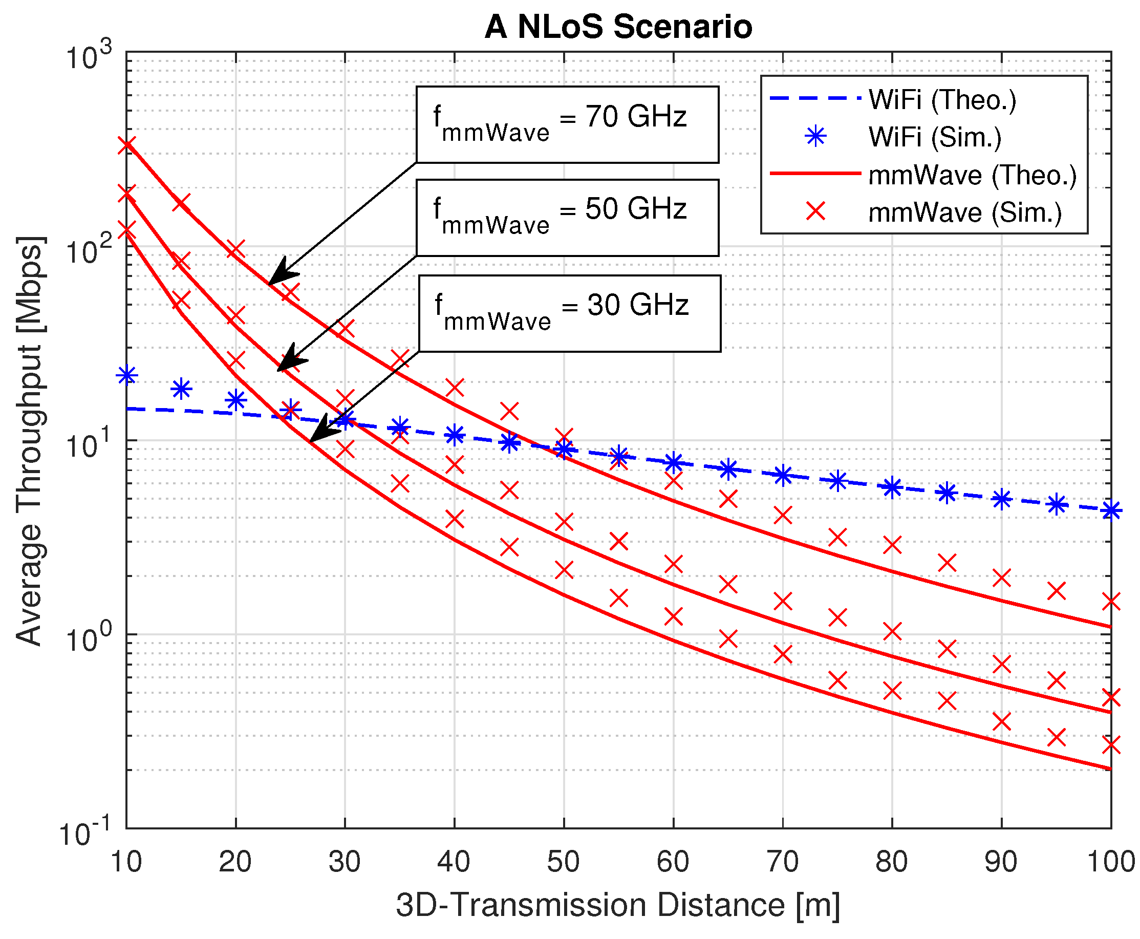
Figure 6 depicts the average throughput (AT) variations versus the transmission distance between vehicles, providing a detailed comparison between WiFi and millimeter waves in an LoS scenario. The results notably highlight that, as the distance between vehicles increases, both millimeter waves and WiFi experience a decrease in average throughput. However, mmWaves exhibit superior AT compared to WiFi, especially with a larger frequency bandwidth. Therefore, the mmWaves demonstrate notably higher throughput than WiFi in an LoS scenario, explained by the advantage of mmWaves that use a wider frequency band compared to WiFi. However, in an NLoS scenario, as depicted in Figure 7, the AT for WiFi bands experiences a slight decrease as the transmission distance increases, whereas mmWaves exhibit a significant decrease with the increase in distance between vehicles. Furthermore, it can be inferred that mmWaves initially demonstrate higher throughput, particularly with a wider frequency band, compared to WiFi. Conversely, WiFi exhibits greater resilience to long distances.
5. Conclusions
In conclusion, the comprehensive analysis conducted in this paper sheds light on a comparison between the performances of WiFi and mmWaves-based V2V communication systems, using realistic stochastic geometry tools. Through rigorous examination encompassing LoS and NLoS scenarios in both 2D and 3D modeling contexts, the corresponding STP and AT expressions for both considered technologies have been derived. Then, numerical results have been provided and analyzed to validate the derived expressions and to investigate the corresponding transmission performances. The results show that the transmission distance and the vehicles’ density have significant impacts on the overall system performances of both technologies. In fact, for a short transmission distance and a low vehicle density, the mmWaves offers a higher transmission performance than that of the WiFi system, However, the WiFi communication systems is more efficient for long transmission distances. Furthermore, the findings underscore that in V2V communications, 3D modeling consistently outperforms 2D simulations, highlighting the crucial role of vertical space in optimizing system performance.
Author Contributions
Methodology, M.R. and A.O.; Software, M.R.; Validation, A.O., S.B., H.C. and R.B.; Investigation, M.R.; Writing—original draft, M.R.; Writing—review & editing, A.O.; Supervision, A.O.; Project administration, R.B. All authors have read and agreed to the published version of the manuscript.
Funding
This research received no external funding.
Conflicts of Interest
The authors declare no conflicts of interest.
Appendix A. Derivation of PLoS Expression for Cases 1&2: p1,2
In this Appendix, we derive the PLoS expression for the cases/event (1 or 2), denoted by .
As explained in Section 2.3, this probability can be expressed as follows:
where and is the PDF of , which is assumed to be uniformly distributed, between the minimum vehicle’s height, denoted by , and the maximum vehicle’s height, denoted by .
Accordingly, the expression of is given by
Consequently, the PDF expression of y can be derived, from the relevant cumulative distribution function (F), as follows:
Now, by using the PDF expression in (A2), the expression of is given by
By using the expressions of and , (A1) can be rewritten as follows:
After evaluating the integrations in (A10), with respect to x and y, and after some simplifications, the final expression of is given by
Appendix B. Derivation of PLoS for Case 3 and 4: p3,4
This Appendix details the derivation of the PLoS expression for cases 3 and 4, denoted by .
According to Section 2.3, the expression can be written as follows:
where , , is the PDF of a, and is the PDF of z, where expression is derived as follows:
Now, by using the PDF expression in (A2), the expression of is given by
By using the expressions of , , , and , (A1) can be rewritten as follows:
After evaluating the integrations in (A10), with respect to x, y, z, and a, and after some simplifications, the final expression of is given by
References
- Abraham, K.S.; Rabin, R.L. Automated vehicles and manufacturer responsibility for accidents. Va. Law Rev. 2019, 105, 127–171. [Google Scholar]
- Sroka, P.; Ström, E.; Svensson, T.; Kliks, A. Autonomous Controller-Aware Scheduling of Intra-Platoon V2V Communications. Sensors 2022, 23, 60. [Google Scholar] [CrossRef]
- Tan, H.; Zhao, F.; Hao, H.; Liu, Z. Evidence for the crash avoidance effectiveness of intelligent and connected vehicle technologies. Int. J. Environ. Res. Public Health 2021, 18, 9228. [Google Scholar] [CrossRef] [PubMed]
- Ivanescu, T.; Yetgin, H.; Merrett, G.V.; El-Hajjar, M. Multi-Source Multi-Destination Hybrid Infrastructure-Aided Traffic Aware Routing in V2V/I Networks. IEEE Access 2022, 10, 119956–119969. [Google Scholar] [CrossRef]
- Ali, R.; Liu, R.; Nayyar, A.; Waris, I.; Li, L.; Shah, M.A. Intelligent Driver Model-Based Vehicular Ad Hoc Network Communication in Real-Time Using 5G New Radio Wireless Networks. IEEE Access 2023, 11, 4956–4971. [Google Scholar] [CrossRef]
- Damaj, I.W.; Yousafzai, J.K.; Mouftah, H.T. Future trends in connected and autonomous vehicles: Enabling communications and processing technologies. IEEE Access 2022, 10, 42334–42345. [Google Scholar] [CrossRef]
- Sepasgozar, S.S.; Pierre, S. Network traffic prediction model considering road traffic parameters using artificial intelligence methods in VANET. IEEE Access 2022, 10, 8227–8242. [Google Scholar] [CrossRef]
- Arena, F.; Pau, G. An overview of vehicular communications. Future Internet 2019, 11, 27. [Google Scholar] [CrossRef]
- Kabil, A.; Rabieh, K.; Kaleem, F.; Azer, M.A. Vehicle to pedestrian systems: Survey, challenges and recent trends. IEEE Access 2022, 10, 123981–123994. [Google Scholar] [CrossRef]
- Hussein, N.H.; Yaw, C.T.; Koh, S.P.; Tiong, S.K.; Chong, K.H. A comprehensive survey on vehicular networking: Communications, applications, challenges, and upcoming research directions. IEEE Access 2022, 10, 86127–86180. [Google Scholar] [CrossRef]
- Alhilal, A.Y.; Finley, B.; Braud, T.; Su, D.; Hui, P. Street Smart in 5G: Vehicular Applications, Communication, and Computing. IEEE Access 2022, 10, 105631–105656. [Google Scholar] [CrossRef]
- Naeem, A.B.; Soomro, A.M.; Saim, H.M.; Malik, H. Smart road management system for prioritized autonomous vehicles under vehicle-to-everything (V2X) communication. Multimed. Tools Appl. 2023, 1–18. [Google Scholar] [CrossRef]
- Wang, M.; Chen, X.; Jin, B.; Lv, P.; Wang, W.; Shen, Y. A novel V2V cooperative collision warning system using UWB/DR for intelligent vehicles. Sensors 2021, 21, 3485. [Google Scholar] [CrossRef] [PubMed]
- Arikumar, K.S.; Prathiba, S.B.; Basheer, S.; Moorthy, R.S.; Dumka, A.; Rashid, M. V2X-Based Highly Reliable Warning System for Emergency Vehicles. Appl. Sci. 2023, 13, 1950. [Google Scholar] [CrossRef]
- Kenney, J.B. Dedicated short-range communications (DSRC) standards in the United States. Proc. IEEE 2011, 99, 1162–1182. [Google Scholar] [CrossRef]
- Chen, X.; Leng, S.; Tang, Z.; Xiong, K.; Qiao, G. A millimeter wave-based sensor data broadcasting scheme for vehicular communications. IEEE Access 2019, 7, 149387–149397. [Google Scholar] [CrossRef]
- Zadobrischi, E.; Dimian, M. Vehicular communications utility in road safety applications: A step toward self-aware intelligent traffic systems. Symmetry 2021, 13, 438. [Google Scholar] [CrossRef]
- Abbasi, I.A.; Shahid Khan, A. A review of vehicle to vehicle communication protocols for VANETs in the urban environment. Future Internet 2018, 10, 14. [Google Scholar] [CrossRef]
- Tahir, M.N.; Leviäkangas, P.; Katz, M. Connected vehicles: V2V and V2I road weather and traffic communication using cellular technologies. Sensors 2022, 22, 1142. [Google Scholar] [CrossRef] [PubMed]
- Giordani, M.; Zanella, A.; Higuchi, T.; Altintas, O.; Zorzi, M. On the Feasibility of Integrating mmWave and IEEE 802.11 p for V2V Communications. In Proceedings of the 2018 IEEE 88th Vehicular Technology Conference (VTC-Fall), Chicago, IL, USA, 27–30 August 2018; IEEE: Piscataway, NJ, USA, 2018; pp. 1–7. [Google Scholar]
- Tahir, M.N.; Katz, M. Performance evaluation of IEEE 802.11 p, LTE and 5G in connected vehicles for cooperative awareness. Eng. Rep. 2022, 4, e12467. [Google Scholar] [CrossRef]
- Sial, M.N.; Deng, Y.; Ahmed, J.; Nallanathan, A.; Dohler, M. Stochastic geometry modeling of cellular V2X communication over shared channels. IEEE Trans. Veh. Technol. 2019, 68, 11873–11887. [Google Scholar] [CrossRef]
- Chetlur, V.V.; Dhillon, H.S. Coverage analysis of a vehicular network modeled as Cox process driven by Poisson line process. IEEE Trans. Wirel. Commun. 2018, 17, 4401–4416. [Google Scholar] [CrossRef]
- Jeyaraj, J.P.; Haenggi, M. Reliability analysis of V2V communications on orthogonal street systems. In Proceedings of the GLOBECOM 2017—2017 IEEE Global Communications Conference, Singapore, 4–8 December 2017; IEEE: Piscataway, NJ, USA, 2017; pp. 1–6. [Google Scholar]
- Chen, R.; Zhong, Z.; Leung, V.C.; Michelson, D.G. Performance analysis of connectivity for vehicular ad hoc networks with moving obstructions. In Proceedings of the 2014 IEEE 80th Vehicular Technology Conference (VTC2014-Fall), Vancouver, BC, Canada, 14–17 September 2014; IEEE: Piscataway, NJ, USA, 2014; pp. 1–5. [Google Scholar]
- Tchouankem, H.; Zinchenko, T.; Schumacher, H. Impact of buildings on vehicle-to-vehicle communication at urban intersections. In Proceedings of the 2015 12th Annual IEEE Consumer Communications and Networking Conference (CCNC), Las Vegas, NV, USA, 9–12 January 2015; IEEE: Piscataway, NJ, USA, 2015; pp. 206–212. [Google Scholar]
- Yi, W.; Liu, Y.; Nallanathan, A. Signal fractions analysis and safety-distance modeling in V2V inter-lane communications. IEEE Commun. Lett. 2020, 25, 1387–1390. [Google Scholar] [CrossRef]
- Jeyaraj, J.P.; Haenggi, M. Cox models for vehicular networks: SIR performance and equivalence. IEEE Trans. Wirel. Commun. 2020, 20, 171–185. [Google Scholar] [CrossRef]
- Petrov, V.; Kokkoniemi, J.; Moltchanov, D.; Lehtomäki, J.; Juntti, M.; Koucheryavy, Y. The impact of interference from the side lanes on mmWave/THz band V2V communication systems with directional antennas. IEEE Trans. Veh. Technol. 2018, 67, 5028–5041. [Google Scholar] [CrossRef]
- Li, K.; Zhou, S.; Tan, G. Performance Analysis of a Reconfigurable-Intelligent-Surfaces-Assisted V2V Communication System. Electronics 2023, 12, 2383. [Google Scholar] [CrossRef]
- Rjab, M.; Omri, A.; Bouallegue, S.; Chamkhia, H.; Bouallegue, R. Modeling and Performance Analysis of mmWave and WiFi Transmissions for V2V Communications. In Proceedings of the 2024 Submitted In 25th IEEE Wireless Communications and Networking Conference (WCNC), Dubai, United Arab Emirates, 21–24 April 20024; IEEE: Piscataway, NJ, USA, 2024. [Google Scholar]
- Abughalwa, M.; Omri, A.; Hasna, M.O. On the average secrecy outage rate and average secrecy outage duration of wiretap channels with rician fading. In Proceedings of the 2018 14th International Wireless Communications & Mobile Computing Conference (IWCMC), Limassol, Cyprus, 25–29 June 2018; IEEE: Piscataway, NJ, USA, 2018; pp. 736–740. [Google Scholar]
- Bachtobji, S.; Omri, A.; Bouallegue, R. Modelling and performance analysis of 3-D mmWaves based heterogeneous networks. In Proceedings of the 2016 International Wireless Communications and Mobile Computing Conference (IWCMC), Paphos, Cyprus, 5–9 September 2016; pp. 72–76. [Google Scholar] [CrossRef]
- Gradshteyn, I.; Ryzhik, I. Tables of Integrals, Series and Products, 7th ed.; Elsevier: New York, NY, USA, 2007. [Google Scholar]
- Omri, A.; Hasna, M.O. Modeling and Performance Analysis of D2D Communications with Interference Management in 3-D HetNets. In Proceedings of the 2016 IEEE Global Communications Conference (GLOBECOM), Washington, DC, USA, 4–8 December 2016; pp. 1–7. [Google Scholar]
- Bachtobji, S.; Omri, A.; Bouallegue, R.; Raoof, K. Modelling and Performance Analysis of mmWaves and Radio-Frequency based 3D Heterogeneous Networks. IET Commun. 2018, 12, 290–296. [Google Scholar] [CrossRef]
Figure 1.
Illustration of a V2V communication example with (a) 3D modeling and (b) 2D modeling.
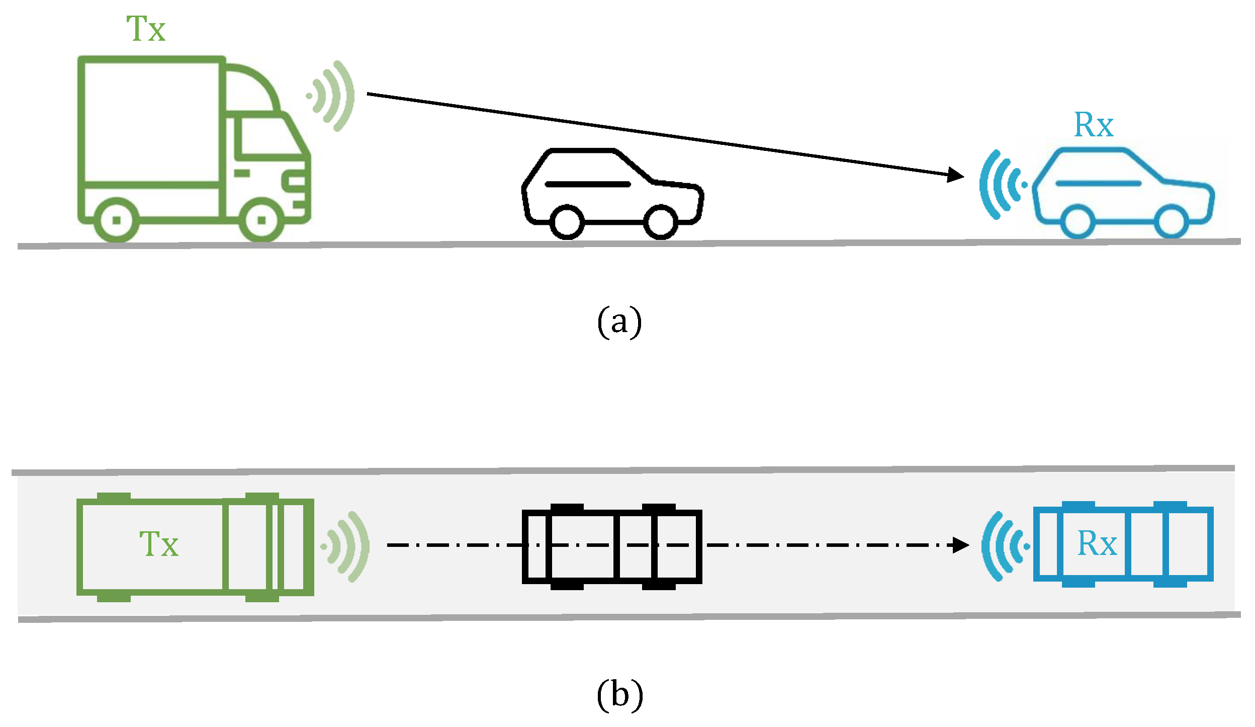
Figure 2.
Illustration of V2V LoS communication scenarios.

Figure 3.
LoS probability vs. transmission distance with different vehicle densities values.
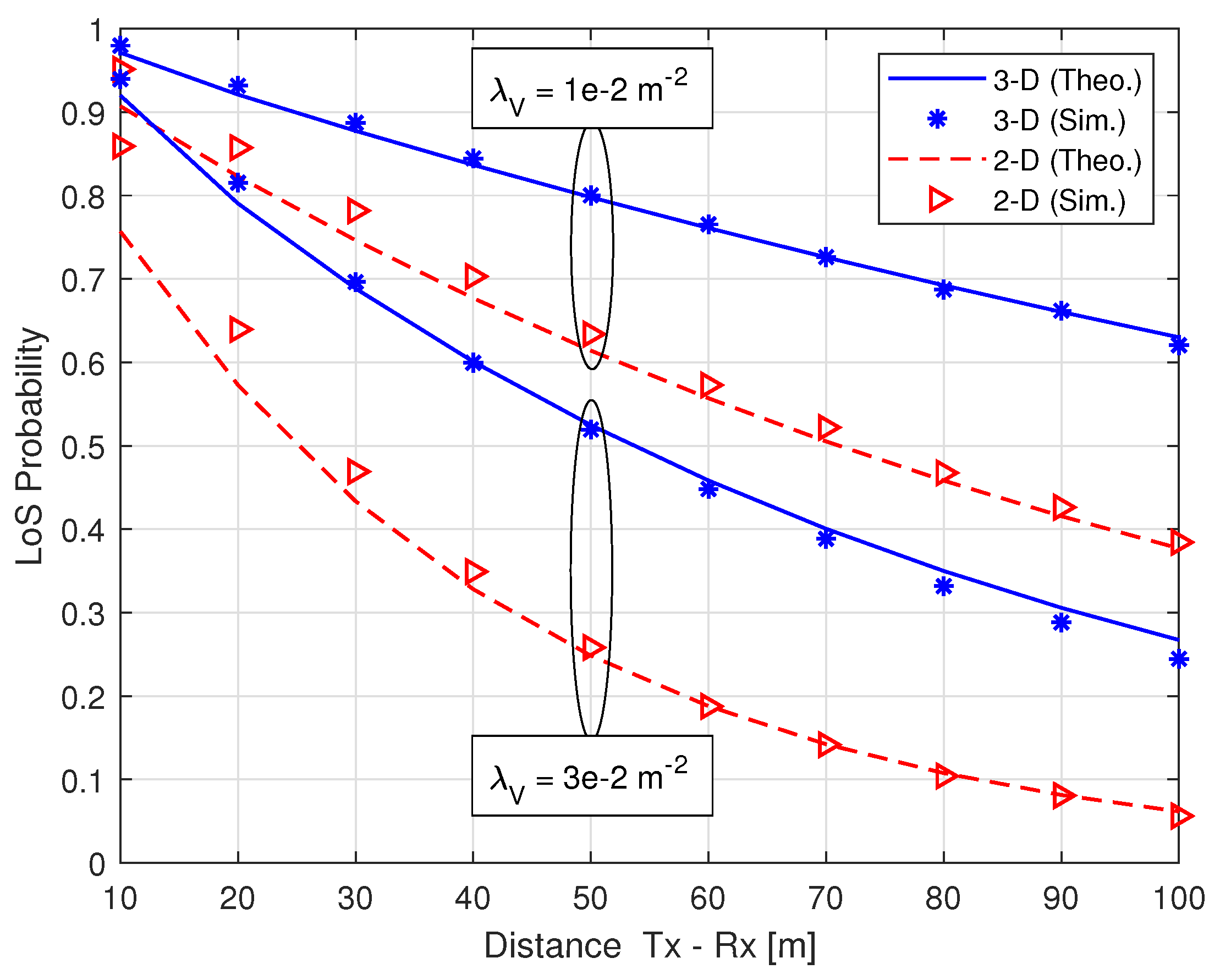
Figure 4.
STP vs. transmission distance in an LoS scenario.
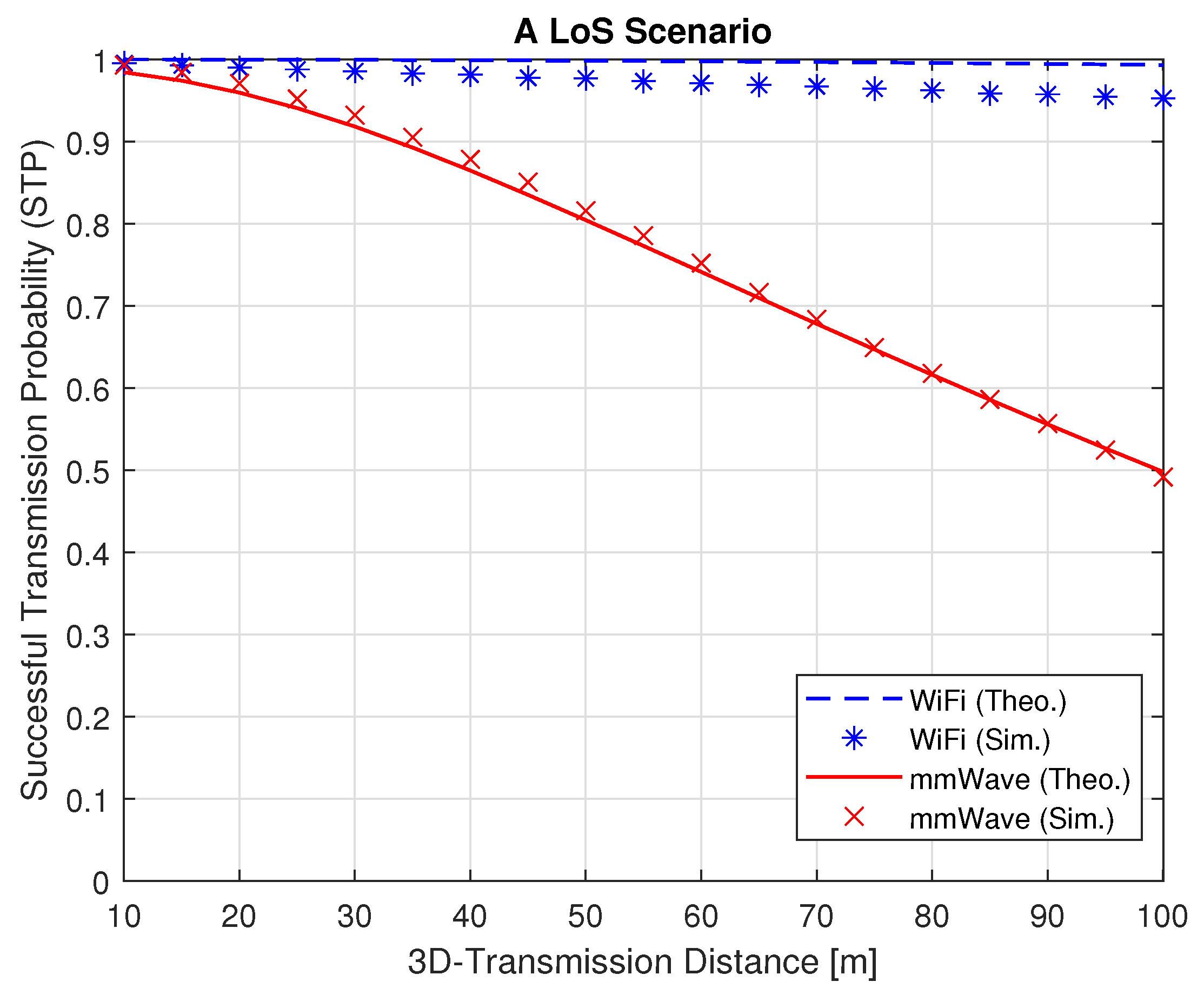
Figure 5.
STP vs. transmission distance in an NLoS scenario.

Figure 6.
Average throughput vs. transmission distance in an LoS scenario.
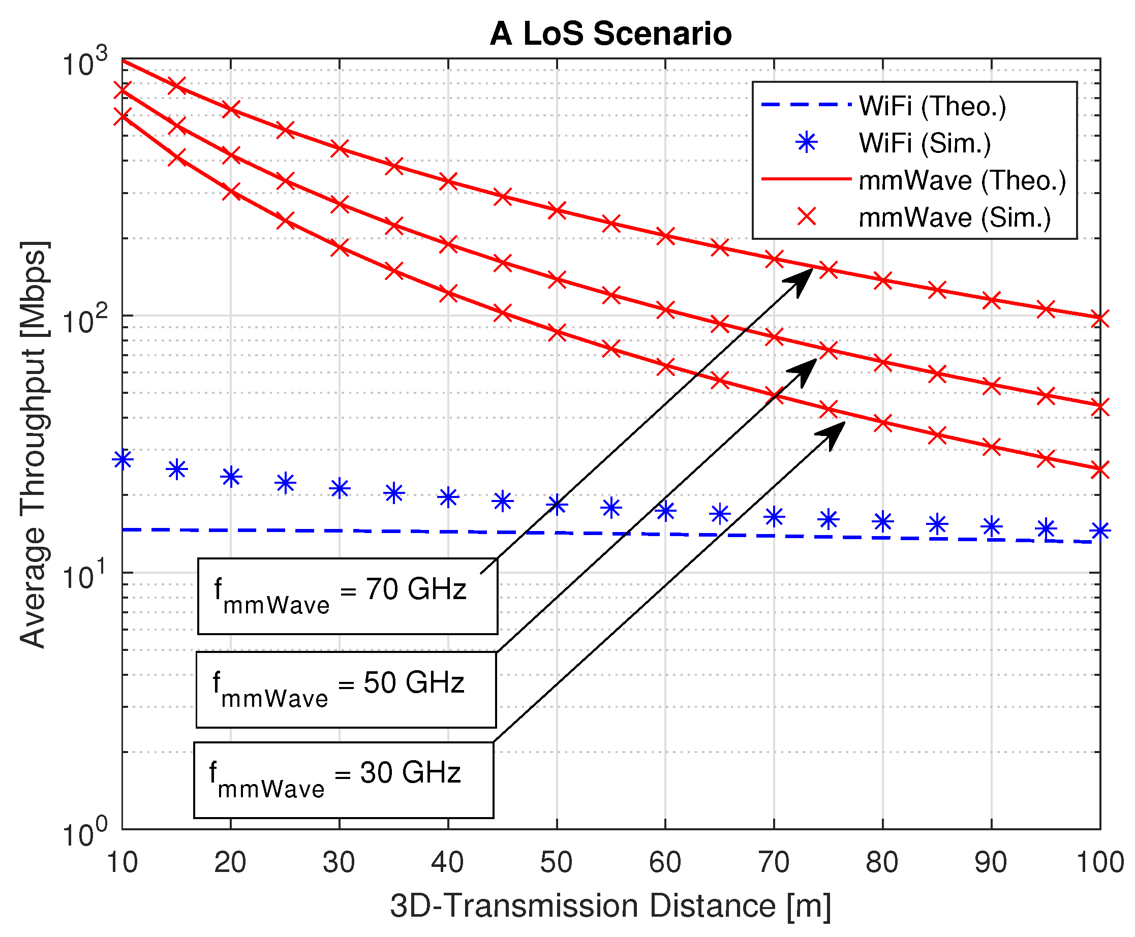
Figure 7.
Average throughput vs. transmission distance in an NLoS scenario.

Table 1.
Related work to V2V system modeling and performance analysis.
| Stochastic Geometry Process | Space Dimension | Channel Model | Performance Analysis Metric | Advantages | Limitations | Ref. |
|---|---|---|---|---|---|---|
| Poisson Point Process | 1-D | Nakagami | SIR | - A low performance analysis complexity. | - A low performance analysis accuracy due to the use of SIR metric and 1D modeling | [23] |
| Rayleigh | SINR | - A comprehensive analysis of the signal fraction (SF)’s performances. | - Complexity of modeling vehicle interactions in realistic vehicle network scenarios. - A low performance analysis accuracy due to the use of Rayleigh channels and 1D modeling. | [27] | ||
| 2-D | Rayleigh | SINR | - Assessment of C-V2X communication performance with flexible mode selection. |
- The 3D distances are not considered. - A low performance analysis accuracy. | [22] | |
| Rayleigh | SIR | - Analyzing vehicle networks in orthogonal road systems. | - The 3D distances are not considered. - A low performance analysis accuracy. | [24] | ||
| Rayleigh | SIR STP | - Enabling characterization of diverse street geometries, including intersections and T-junctions. | - A low vehicles’ 2D distribution accuracy - A low performance analysis accuracy. | [28] | ||
| Rayleigh Rice | SINR | - Highlighting the buildings’ role in mitigating co-channel interference, improving V2V communication reliability at urban intersections. | - The 3D distances are not considered. - A low performance analysis accuracy. | [26] | ||
| 3-D | Nakagami | SINR Link Capacity | - A 3D representation of vehicular spatial position. | - A high-complexity performance analysis. | [29] | |
| Matern Hard-Core Point Processes | 1-D | Rayleigh | SINR | - The use of an accurate stochastic geometry process. | - A low performance analysis accuracy due to the use of Rayleigh channels and 1D modeling. | [30] |
Table 2.
The used notations throughout the paper.
| Notation | Definition |
|---|---|
| The ’s height | |
| The ’s height | |
| The threshold height | |
| a | The distance between and a given vehicle V |
| The obstacle vehicle’s height | |
| The maximum vehicle’s height | |
| The minimum vehicle’s height | |
| d | The 2D distance between and |
| r | The 3D distance between and |
Table 3.
The different conditions of LoS and NLoS scenarios.
| Case | Condition | Scenario |
|---|---|---|
| 1 | LoS | |
| 2 | LoS | |
| 3 | LoS | |
| 4 | LoS | |
| 5 | NLoS | |
| 6 | NLoS | |
| 7 | NLoS | |
| 8 | NLoS |
Table 4.
The values of the simulation parameters.
| Parameter | Value |
|---|---|
| N | 150 |
| 5 | |
| 5 GHz | |
| GHz | |
| 2 MHz | |
| 100 MHz | |
| 10 [dB] | |
| [dB] | |
| 2 | |
| 3 | |
| 2 | |
| C | |
| 1 | |
| 2 | |
| 1 | |
| 1 | |
| 2 | |
| 1 | |
Disclaimer/Publisher’s Note: The statements, opinions and data contained in all publications are solely those of the individual author(s) and contributor(s) and not of MDPI and/or the editor(s). MDPI and/or the editor(s) disclaim responsibility for any injury to people or property resulting from any ideas, methods, instructions or products referred to in the content. |
© 2024 by the authors. Licensee MDPI, Basel, Switzerland. This article is an open access article distributed under the terms and conditions of the Creative Commons Attribution (CC BY) license (https://creativecommons.org/licenses/by/4.0/).
Share and Cite
MDPI and ACS Style
Rjab, M.; Omri, A.; Bouallegue, S.; Chamkhia, H.; Bouallegue, R. Modeling and Performance Analysis of mmWave and WiFi-Based Vehicle Communications. Electronics 2024, 13, 1344. https://doi.org/10.3390/electronics13071344
AMA Style
Rjab M, Omri A, Bouallegue S, Chamkhia H, Bouallegue R. Modeling and Performance Analysis of mmWave and WiFi-Based Vehicle Communications. Electronics. 2024; 13(7):1344. https://doi.org/10.3390/electronics13071344
Chicago/Turabian StyleRjab, Mohamed, Aymen Omri, Seifeddine Bouallegue, Hela Chamkhia, and Ridha Bouallegue. 2024. "Modeling and Performance Analysis of mmWave and WiFi-Based Vehicle Communications" Electronics 13, no. 7: 1344. https://doi.org/10.3390/electronics13071344
Note that from the first issue of 2016, this journal uses article numbers instead of page numbers. See further details here.