

Population Game-Assisted Multi-Agent Reinforcement Learning Method for Dynamic Multi-Vehicle Route Selection

Software School, East China Jiaotong University, Nanchang 330013, China
*
Author to whom correspondence should be addressed.
Electronics 2024, 13(8), 1555; https://doi.org/10.3390/electronics13081555
Submission received: 17 March 2024
/
Revised: 8 April 2024
/
Accepted: 12 April 2024
/
Published: 19 April 2024
(This article belongs to the Topic Cooperative Localization, Optimization and Control of Networked Autonomous Systems: Theories, Analysis Tools and Applications)
Abstract
:To address urban traffic congestion, researchers have made various efforts to mitigate issues such as prolonged travel time, fuel wastage, and pollutant emissions. These efforts primarily involve microscopic route selection from the vehicle perspective, multi-vehicle route optimization based on traffic flow information and historical data, and coordinated route optimization that models vehicle interaction as a game behavior. However, existing route selection algorithms suffer from limitations such as a lack of heuristic, low dynamicity, lengthy learning cycles, and vulnerability to multi-vehicle route conflicts. To further alleviate traffic congestion, this paper presents a Period-Stage-Round Route Selection Model (PSRRSM), which utilizes a population game between vehicles at each intersection to solve the Nash equilibrium. Additionally, a Period Learning Algorithm for Route Selection (PLA-RS) is proposed, which is based on a multi-agent deep deterministic policy gradient. The algorithm allows the agents to learn from the population game and eventually transition into autonomous learning, adapting to different decision-making roles in different periods. The PSRRSM is experimentally validated using the traffic simulation platform SUMO (Simulation of Urban Mobility) in both artificial and real road networks. The experimental results demonstrate that PSRRSM outperforms several comparative algorithms in terms of network throughput and average travel cost. This is achieved through the coordination of multi vehicle route optimization, facilitated by inter-vehicle population games and communication among road agents during training, enabling the vehicle strategies to reach a Nash equilibrium.
1. Introduction
In recent years, as urbanization advances worldwide, the number of urban vehicles is also constantly rising, resulting in a gradual increase in traffic congestion, which has become a significant factor impacting the efficiency of traffic flow. The congestion reduces vehicle traveling speed, causes delays, and leads to increased tailpipe emissions, fuel consumption, adverse health effects on residents, and safety risks, resulting in significant socio-economic losses [1]. Consequently, addressing the issue of traffic congestion through the application of traffic models and algorithms to enhance traffic efficiency [2] in urban road networks has garnered significant attention within academic circles. In this context, route selection [3] algorithms play a crucial role.
The existing methods can be categorized into microscopic route selection from a single-vehicle perspective, multi-vehicle route selection using traffic information and historical data, and coordinated route optimization based on game theory. The microscopic route selection methods, which concentrate on the single-vehicle perspective, encompass a range of conventional methods such as Dijkstra’s algorithm [4], A* algorithm [5], and the artificial potential field method [6]. Furthermore, there are graphical methods like the stochastic roadmap method [7] and the fast search random tree method [8], as well as swarm intelligence algorithms such as genetic algorithms [9], ant colony algorithms [10], and particle swarm algorithms [11]. However, these single-vehicle route selection algorithms often prove ineffective when applied to multi-vehicle route selection. This ineffectiveness stems from the fact that these algorithms only consider the processing of road information by a single vehicle, which does not account for the impact of one vehicle on the passage of others. Consequently, congestion can easily develop on the initially optimal route, resulting in secondary congestion.
Scholars have suggested multi-vehicle route optimization based on traffic flow information and historical data to minimize secondary congestion. Some methods acquire network information such as congestion, accidents, and roadworks to understand traffic conditions [12], or involve quantifying road congestion and using reinforcement learning to make decisions [13]. Despite their negotiating nature, these methods have limited vehicle-to-vehicle interaction and may lack generalization capabilities. To enhance group interest considerations, scholars have introduced coordinated multi-vehicle route optimization based on game theory. Examples include the population game [14] and the Stackelberg game [15]. While these methods efficiently determine optimal vehicle strategy combinations, their computational efficiency decreases significantly when applied to high-dimensional data structures.
The above-mentioned methods are effective in alleviating congestion and enhancing traveling efficiency within urban road networks to some extent. Nevertheless, several limitations exist. Some methods lack interaction between vehicles, leading to low road utilization. Additionally, certain methods are not sufficiently responsive in highly dynamic traffic environments, causing difficulty in maintaining optimal strategies. Moreover, some methods mandate excessive details regarding vehicle interactions, thus reducing computational efficiency. Furthermore, in most existing methods, route selection only takes travel time into account, while the evaluation index is overly simplistic.
The multi-vehicle route selection problem diverges from single-vehicle route selection as it aims to ameliorate congestion and reduce overall traveling cost for all vehicles. A large number of vehicles choosing the optimal route under the non-negotiated method easily causes secondary congestion to occur. Therefore, resolving the multi-vehicle route selection predicament necessitates the coordination of vehicle strategies, aiming to exchange individual optimums for a group optimum. Moreover, in scenarios with extensive road network traffic, the dynamic nature of decision making and the real-time adjustment of multi-vehicle routes become imperative, as failure to do so could trigger the new congestion.
This paper proposes a multi-stage population game route selection model to balance traffic flow on the road, alleviate congestion in the entire road network. Building on this model, the paper introduces a Period Learning Algorithm for Route Selection based on a multi-agent deep deterministic strategy gradient [16] to enhance the dynamics, collaboration, and learning ability of the method. The algorithm involves a population game occurring at regular intervals between vehicles approaching the same intersection. Given the drivers’ bounded rationality [17], vehicles are categorized into multiple populations, and the Nash equilibrium is determined through repetitive strategy selection in a finite number of stages and optimization using mixed strategies [14]. In the Period Learning Algorithm for Route Selection, same-direction roads between adjacent intersections are represented as road agents, using an actor–critic network structure [18] with centralized training and distributed execution. The algorithm is divided into three periods. In the first period, road agents learn from their experiences solely based on the outcomes and gains of the population game. In the second period, the agent initializes vehicle strategies, replacing random initialization to expedite game convergence. In the third period, the agent strategies are directly employed as the executed vehicle strategies. In this period, the learning algorithm capitalizes on the multi-agent system’s high learning starting point through its experience from the population game, while also continuing to learn and provide direct decisions for the vehicles.
The main contributions of this paper are described as follows.
- A Period-Stage-Round Route Selection Model (PSRRSM) is introduced to precisely address the Nash equilibrium by dividing vehicle populations at each intersection. It uses a multi-stage game strategy to coordinate the determination of optimal routes for multiple vehicles.
- The Period Learning Algorithm for Route Selection (PLA-RS) uses population game data from PSRRSM to help road agents learn more quickly, improving the accuracy and efficiency of dynamic route selection for vehicles. Importantly, the PLA-RS takes into account multifaceted travel costs in its considerations.
- The Vehicle Multi-stage Population Game Algorithm (VMPGA) is crafted to furnish game decisions for vehicles at each intersection in the Period Learning Algorithm for Route Selection (PLA-RS). It plays a crucial role in substantially optimizing vehicle routes and enhancing coordination capabilities, serving as an informative source for PLA-RS.
The rest of this paper is organized as follows. Section 2 presents related works, followed by Section 3, which explains the Period-Stage-Round Route Selection Model and the weighted definition of vehicle travel cost. Section 4 outlines the Period Learning Algorithm for Route Selection. This is followed by Section 5, which discusses the validation of the algorithm’s performance through experiments. Finally, Section 6 concludes the paper and offers an outlook for future work.
2. Related Works
Misztal et al. [19] proposed the iterative local search algorithm (ILS) for a variant of the Vehicle Routing Problem (VPR) and made the Sawp (2-1) algorithm work with a single perturbation mechanism, which is used to increase the search area and improve the quality of the returned solution, and can be used to solve a large group of vehicle route problems. Šedivý et al. [20] discussed the possible application of the solver optimization module in solving the single-loop traveling salesman problem and demonstrated the corresponding algorithms, which not only significantly reduced the distance traveled, but also reduced the time required to design the route. Stopka et al. [21] applied opted operations research methods to the urban logistics transportation and distribution problem, including the Clarke–Wright algorithm, Mayer algorithm, and nearest neighbor algorithm, which dramatically improved the truck capacity utilization. Paisarnvirosrak et al. [22] proposed a method combining the firefly algorithm with a forbidden search algorithm for solving the Vehicle Routing Problem with Time Windows (VRPTW), which significantly reduces the fuel consumption, the number of vehicles required for transportation, the consumption of money, and the greenhouse gas emissions. The above heuristic algorithms and swarm intelligence algorithms can alleviate traffic congestion and reduce the cost of travel time, distance, fuel, etc., to some extent. However, limitations in vehicle negotiation make them difficult to use in large-scale route selection problems.
Zhang et al. [23] introduced the concept of vehicle fairness care to improve coordination between vehicles and reduce travel costs. They developed a coordinated route model based on an asymmetric congestion game to achieve this goal. Lejla et al. [24] proposed a cooperative behavioural strategy for self-driving vehicles by using a game theory approach, which can effectively solve the turn entry problem and shorten the waiting time. Lin et al. [25] proposed the Social Vehicle Route Selection (SVRS) algorithm, which combines historical and current drive information and uses game evolution method to calculate the optimal routes. Tai et al. [26] modeled vehicles by studying two-dimensional metacellular automata to better coordinate vehicles in dense road networks with route greedy updates of appropriate frequency. Tanimoto et al. [27] explored the route selection problem using a metacellular automata simulation that coincides with evolutionary game theory, modeling the interaction between vehicles as an n-chicken game and solving this game by providing appropriate information to the driver agents, which in turn alleviates urban traffic congestion. The above game theory methods can use either collaborative or adversarial approaches to make each game participant reach the optimal strategy. However, while good route decisions can be made, the game theory method has considerable complexity, and its role is limited in scenarios where the dynamic requirement and the congestion level are high. At the same time, reinforcement learning-based route selection methods require a long training cycle while possessing efficient decision-making capability. Reinforcement learning methods combined with game theory have been applied in a variety of fields, but rare in the field of path selection. Whether it can surpass the decision-making effect of separate game theory methods or reinforcement learning methods is a question worth studying.
Mortaza et al. [28] proposed a route selection model based on the Multi-agent Reinforcement Learning (MARL) algorithm to assess the impact of multiple traffic factors on vehicle delays. The model examines the weights of different components of the road network environment, including weather, traffic, and road safety, in order to determine the prioritized routes for vehicles. To enhance the utilization of historical data, Li et al. [29] incorporated a heuristic search strategy into the enhanced Q-Learning algorithm to accelerate the learning process and reduced the search space by constraining the range of direction angle variation. Liu et al. [30] proposed to use the Dyna framework to improve the speed of the decision making, and used the Sarsa algorithm as a routing strategy to improve the security of the algorithm, and finally combined the two to propose a Dyna-Sa algorithm. Zhou et al. [31] proposed a decentralized execution order scheduling method based on multi-agent reinforcement learning for a large-scale order scheduling problem, where all the Agents work independently guided by a joint policy evaluation. Mona Alshehri et al. [32] proposed an extension of the graph evolutionary algorithm to make it more suitable for solving coordinated multi-agent route selection tasks in dynamic environments.
In order to improve the learning efficiency of the algorithm, Nazari et al. [33] proposed an end-to-end framework for solving vehicle routing problems using deep reinforcement learning. Li et al. [34] proposed an DRL method based on an attention mechanism, which contains a vehicle selection decoder considering heterogeneous fleet constraints and a node selection decoder considering route construction. Nai et al. [35] proposed a mixed-strategy gradient actor–critic model with a stochastic escape term and a filtering operation, using a model-driven approach to ensure the convergence speed of the whole model. Berat et al. [36] proposed a synergistic combination of deep reinforcement learning and hierarchical game theory as a modelling framework for driver behaviour prediction in motorway driving scenarios. Reinforcement learning methods, including those discussed above, leverage historical data to enhance vehicle decision making and coordination flexibility and efficiency. Although these methods demonstrate some degree of adaptability and extensibility, they have not made significant strides in addressing complex sequential decision-making problems. Moreover, challenges such as prolonged learning cycles, low data utilization, and limited generalization abilities persist.
In summary, the existing vehicle route selection methods for urban road networks have limitations such as insufficient dynamics, slow convergence, and single driving cost factor. In addressing the complex challenges presented by the vast data dimension, high dynamics, continuous action space and state space of multi-vehicle route selection in urban road networks, this paper introduces the PSRRSM model. This model is based on population game and multi-agent deep reinforcement learning, enabling vehicles within the enter edges of each intersection to dynamically select routes. From this model, the paper derives the PLA-RS route selection algorithm, designed to enhance the reliability and efficiency of multi-vehicle decision making. Additionally, a route cost calculation method is proposed, considering factors such as energy consumption, environmental pollution, and driver preference. This holistic approach aims to disperse traffic flow, ease traffic congestion, and optimize travel time in urban road networks.
3. Period-Stage-Round Route Selection Model
Existing route selection methods often do not fully consider the dynamics of traffic conditions in urban road networks, nor do they fully consider the degree of vehicle-to-vehicle interaction. In order to better coordinate multi-vehicle route decisions in urban road networks and further reduce road network congestion, this paper proposes the Period-Stage-Round Route Selection Model (PSRRSM), as shown in Figure 1. This model offers coordinated route selection decisions for large number of vehicles within urban road networks. It facilitates the continuous learning of the relationship between road states, vehicle strategies, and game benefits by road agents. In doing so, it allows for the ongoing reduction of the average travel cost in iterations, resulting in time, distance, and fuel savings for travelers, while simultaneously optimizing global benefits. Section 3.1 of this chapter specifically describes the model definition of PSRRSM, and Section 3.2 describes the specific way in which utility is calculated.
3.1. Problem Model
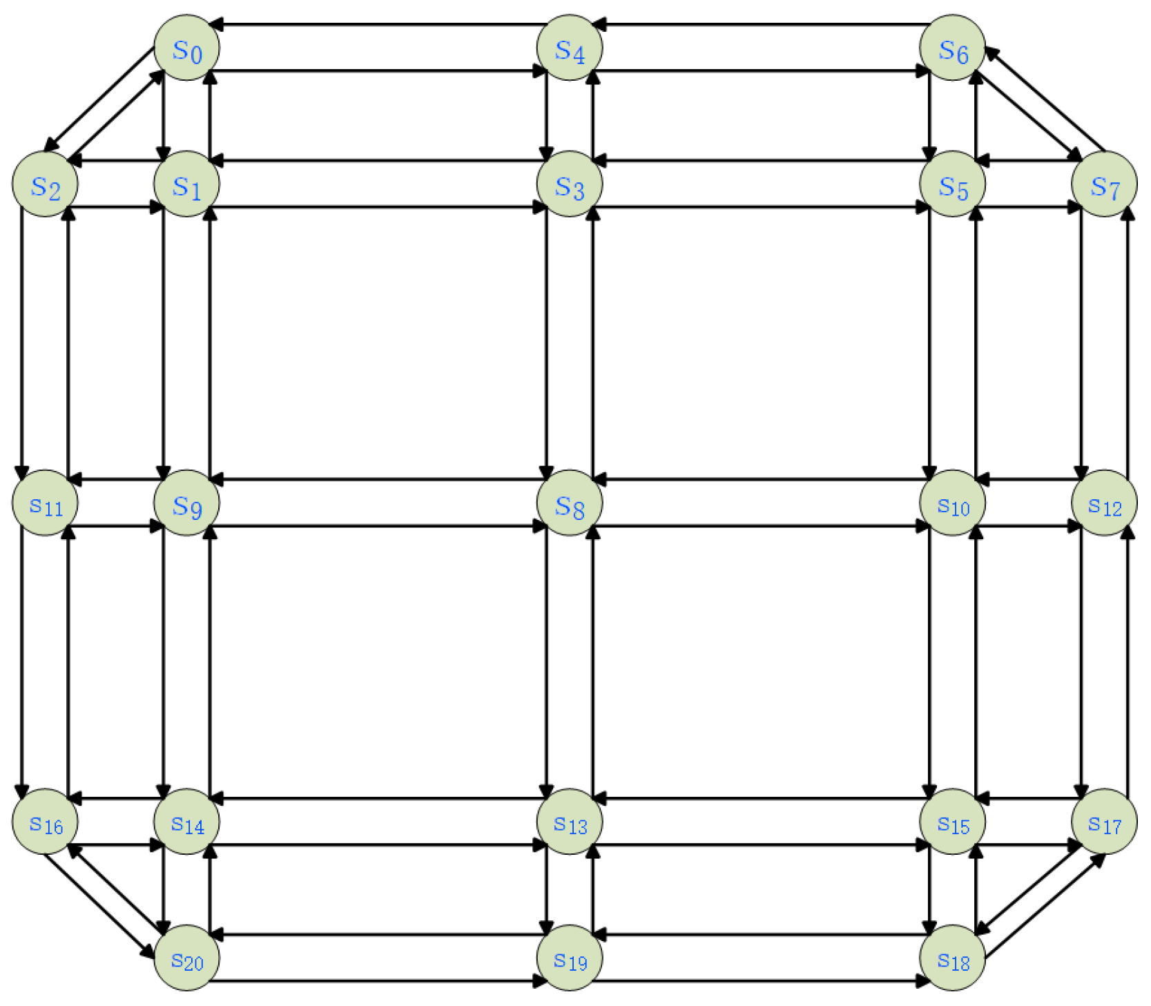
The urban road network model comprises nodes and edges. Nodes symbolize intersections, while edges represent roads. Essentially, it is a weighted directed graph , where S represents the intersections and L represents the edges (roads), as illustrated in Figure 2. The number of intersections in an urban road network is denoted by and the number of roads is . Roads are also called segments. denotes the ith intersection. For any two neighbouring intersections and , a road from directly to is denoted by . Note that and do not necessarily exist at the same time, due to the presence of one-way roads in the road network. Use to denote the set of roads adjacent to and with direction towards , i.e., the set of enter edges, and to denote the set of roads adjacent to and with direction away from , i.e., the set of off edges. For example, the set of enter edges for intersection in Figure 2 is and the set of off edges is . Each edge owns a road agent .
In the urban road network described by the directed graph , the set of all vehicles is denoted as V, and any vehicle . The original edge and destination edge of vehicle v are denoted by and , respectively. At moment t, the set of edges that vehicle v has already passed is denoted by , and the current edge is denoted by . When a vehicle, denoted as v, is positioned at edge , it engages in estimating the total cost of the available routes at the current location. Furthermore, the vehicle takes part in the collective decision-making process along with all other vehicles at the enter edges of the upcoming intersection. Subsequently, based on the collective decision, the vehicle selects one of the off edges of the intersection as its next route. This selected off edge is referred to as , representing the subsequent edge chosen by vehicle v. Denote by the pure strategy chosen by the vehicle v, assuming that the intersection ahead is , as shown as follows:
Denote by the set of optional pure strategies for the vehicle v currently located at one enter edge of the intersection , as shown as follows:
where is an arbitrary off edge of the intersection .
The set consisting of all vehicles on the enter edges of intersection is called the decision unit of intersection and is denoted by , as shown as follows:
Denote by whether the current pure strategy of vehicle v selects the off edge . If yes, then ; if no, then . The strategies selected by the vehicles in may not be all the same, which implies that they do not select all the same off edge either. Denote the proportion of vehicles included in choosing different strategies by the road vehicle state , as shown as follows:
where denotes the proportion of vehicles included in that choose the strategy to all vehicles in .
Denote by the intersection vehicle state the proportion of vehicles included in that choose different strategies when divided by enter edges, as shown as follows:
In order to enrich the travel cost considerations and take into account multiple terms to be optimized, the travel cost of an edge is defined as a weighted sum of time cost, distance cost, fuel cost, emission cost, and driver preference values. Taking edge as an example, the weighted sum of the travel cost of the edges is formulated as shown as follows:
In formula (6), is the time cost of , is the distance cost of , is the fuel cost of , is the pollution cost of , and is the driver preference cost of . are the weighting coefficients, which satisfy the constraint . Using to represent any possible finite route in the urban road network, the travel cost of is the sum of the travel costs of the included edges, as shown as follows:
The multi-vehicle route selection problem in urban road networks presents several unique characteristics. Firstly, the urban road networks are characterized by a high density of vehicles, especially at intersections. The presence of numerous vehicles at each intersection complicates the traffic scenario. Secondly, the movement of each vehicle influences the travel cost of the road it is on, subsequently impacting the costs associated with the routes of other vehicles. Furthermore, as the number of vehicles increases, this influence accumulates, thereby altering the optimal routes of the vehicles. The population game is a kind of game that iteratively seeks for an equilibrium solution, which is applicable to the scenarios that satisfy the following conditions: the existence of a large number of self-decision-making game players; the strategy of a single game player has a small impact on the payoff of other game players; and the payoff of a single game player is determined by the distribution of the strategies of all the game players, including itself. In multi-vehicle route selection on an urban road network, using vehicles as game players and thus using the population game approach satisfies these three conditions and theoretically reduces the average travel cost. The players of each game are all the vehicles included in the decision unit , and the vehicles included in each of these enter edges are a population.
At the onset of each time step, vehicles located at the entrance edges of each intersection are organized into decision units () to engage in multi-vehicle decision-making through population game-based approaches. This aims to address the overall congestion in urban road networks, enhance road access efficiency, and lower the average multi-vehicle travel cost within the framework of comprehensive travel cost. During this process, enter edge agents undergo learning and training. The objective is to ensure that each vehicle’s chosen strategy is optimal, given the unchanged strategies of other vehicles within the decision unit, ultimately reaching a Nash equilibrium within each decision unit. On the time line, a certain decision frequency is guaranteed so that all vehicles in the road network can participate in multi-vehicle decision making on every edge they pass through, thus minimising congestion on the urban road network. The optimization goal of the Period-Stage-Round Route Selection Model is as shown as follows:
where denotes the route determined by the current pure strategy for vehicle v. denotes the current shortest route from to as defined by the integrated travel cost.
3.2. Utility Calculation
When participating in multi-vehicle decision making at an intersection, all vehicle on the enter edges serves as the decision unit. Vehicle v selects an enlightened route, denoted as , which includes the current edge and the next edge. This selection is made based on a strategy and the integrated travel cost calculated after each strategy is chosen. Where the integrated travel cost is a weighted sum of time, distance, fuel, pollution, and driver preference. This section describes how these travelling sub-costs are estimated. According to the BPR (Bureau of Public Roads) formula, the time cost for any edge in the road network in the population game occurring at intersection is calculated as follows:
where is the maximum permissible speed of edge , and is the maximum capacity of edge . , are the parameters. , are the arbitrary neighbouring intersections.
The prediction of the time cost for intersection involves the estimation of the number of vehicles on the off edge , based on the current pure strategy of each vehicle on the enter edges. Additionally, the prediction also entails estimating the number of vehicles on the other edges using the static current number of vehicles . The formula for predicting the number of vehicles on the off edge is shown as follows:
where denotes the current number of vehicles on edge and denotes the current number of vehicles on decision unit , which is equivalent to .
The distance cost is the length of the edge.
Fuel cost is proportional to distance cost. Fuel cost are calculated as follows:
where is the current total fuel consumption of vehicle v and is the current total mileage of vehicle v.
Pollution cost is proportional to the time cost. The pollution cost is calculated as follows:
where is the current total emission of vehicle v and ) is the current total travel time of vehicle v. Note that only the distance cost above is a constant and accurate value, while the formulas for time, fuel, and pollution costs are estimates of future costs. Moreover, the time cost is the same for all vehicles at the same moment, while the fuel and pollution costs are related to each vehicle’s own properties.
Driver preference costs simulate individual subjective estimates of the sum of the four costs of time, distance, fuel, and pollution by different drivers, and require a balance between certainty and uncertainty. The driver preference cost is calculated as follows:
where is the variance and denotes random values taken from a normal distribution determined by the given mean and variance. Cost estimates for the same driver for the same edge at the same moment are not generated repeatedly.
4. Period Learning Algorithm for Route Selection
In order to combine the accuracy of game-theoretic equilibrium solutions and the convergent and generalization ability of multi-agent reinforcement learning methods, this paper introduces a vehicle population game and a road multi-agent system. While the vehicles contained in the decision unit participate in the game, the corresponding road agents learn according to the position distribution of the vehicles and the outcome state of the game—i.e., the proportion of vehicle strategies. After extensive training, the strategies provided by the road agents result in a total benefit that approaches or exceeds the effect of the population game. This can effectively reduce the average cost of travel for multiple vehicles and alleviates congestion in the urban road network. Section 4.1 describes the method architecture of the Period Learning Algorithm for Route Selection based on the Period-Stage-Round Model, and Section 4.2 describes the specific implementation process of the Period Learning Algorithm for Route Selection.
4.1. Method Architecture
In order to use the vehicles population game to assist the learning of road agents in order to improve the final decision making, the overall training process of the algorithm is divided into three periods in this paper. In each period, the training method, the training degree, and the degree of participation in decision making of the agents are different. This process is called “period learning”. The overall architecture of the Period Learning Algorithm for Route Selection is as follows.
The Vehicle Multi-stage Population Game Algorithm is a sub-algorithm within the Period Learning Algorithm for Route Selection. It operates by enabling the vehicles in the decision unit to initially obtain a strategy, and then continuously refine this strategy through multi-stage iteration. This iterative process allows the vehicles to arrive at an equilibrium solution, with termination occurring under one of two conditions: the Nash equilibrium or when the maximum number of stages is reached. In the first period, the initial strategies of the vehicles are randomly generated, as in the general application of the population game; in the second period, the initial strategies of the vehicles are generated by the road agent of the edge where they are located, in order to improve the convergence rate of the game. During the first and second periods, the equilibrium solution prompts the execution of each vehicle strategy in the following time step. Subsequently, the recorded data are stored in the replay buffer of the road agents. It including the number of vehicles on each edge, the proportion of strategies, the cumulative vehicle payoffs, and the number of vehicles on each edge at the conclusion of the subsequent time step.This facilitates the sampling and training process for the road agents. In the third period, the road agents having undergone comprehensive training through the Period Learning Algorithm for Route Selection, transition to the stage where they are empowered to make direct decisions. Consequently, they execute actions by directly implementing the initial strategies, rendering the Vehicle Multi-stage Population Game Algorithm inactive during this period.
The Period Learning Algorithm for Route Selection uses the distribution of the number of vehicles, the proportion of strategies, and the payoffs of the game under the equilibrium solution of the game as training data for road agents. By employing neural networks, the algorithm optimizes the initial strategies of the population game during the convergence of its parameters, thus enhancing the convergence rate of the game. With improved convergence rate, the empirical data provided for the road agents also improves. By iteratively repeating this process, both the convergence speed and convergence rate of the road agents and the population game are significantly enhanced. This aims to enable the road agents to independently achieve the decision-making effect of the population game and to continue learning in order to maintain the decision-making effect. We denote the deep reinforcement learning model of road agents in this paper by tuple . Where denote the number of agents, joint state, observation, joint action, reward function, and decay factor, respectively.
- N: The number of agents, which corresponds to the number of roads. Agent is also known as road agent . .
- S and O: The observation of agent is the vector consisting of the number of vehicles of all neighbouring edges, where the edges . is the set of edge ’s neighbouring edges. The set of neighbouring edges is defined as follows:In Figure 2, the set of neighbouring edges of is . The neighbouring edges of an edge include itself. ’s observation state at the ltth time step is denoted by . The joint state is a matrix consisting of the observations of all agents.
- A: The action of agent at time step is defined as the proportion of strategy selection for the vehicle contained in the corresponding edge . In this algorithm, there exists online action and target action , where the former is generated by the agent, and the latter is the action that the agent needs to learn, and also the proportion of the strategy that the vehicle actually executes. In different periods of this algorithm, the relationship between and is different. In period 1, the Agent does not generate and converts the Nash equilibrium generated by the game to ; in period 2, the agent’s actor network generates , which is used to optimize the initial strategies of the vehicles in order to improve the convergence rate of the game, but the used for learning is still converted from the Nash equilibrium; in period 3, , and the vehicle directly executes the strategy given by the agent.Distribution of actions: convert from proportional to integer according to the number of vehicles on edge . Following the pairing principle, when vehicle v participates in the game at intersection , if the off edge chosen by satisfies , then , . When the remaining vehicles cannot be matched with the remaining strategies, a random distribution is performed. Distribution is complete when all go to zero.
- R: The reward of agent at time step is defined as the opposite of the sum of travel costs of the vehicles included in the corresponding edge , i.e., .
- : Decay factor that determines the importance of the rewards obtained from one learning. As time progresses, the importance of rewards produced later decreases.
With the road agents and the training method, the model can be made to learn the relationship between the current state, the strategy, the next state and the reward received. The road agents completes their communication in the centralized training of the actor and critic networks and makes decisions using only local observations, with the actor network generating the actions. In the first period, the road agents focus on learning the equilibrium solution generated by the population game in order to achieve intersection vehicle states that are close to the equilibrium solution. During the second period, the intersection vehicle states are derived by applying the actions generated by the road agents, which serve to initialize the strategy distribution of the vehicles. This approach aims to yield a significant improvement in the rate and speed of convergence of the population game, while the agents continue training. Subsequently, when the multi-agent learning process reaches a certain level of stability, it transitions into the third period. In this period, the vehicles no longer rely on reaching an equilibrium solution through the game, but rather directly execute the strategy distribution provided by the road agents. This transition represents an evolution in the dynamic interaction between the road agents and the vehicles, as their strategic decision making becomes more streamlined and efficient. The training process of the agents is shown in Figure 3.
4.2. Period Learning Algorithm for Route Selection Implementation
In order to make the collaboration and decision making between vehicles at each enter edge of the intersection more efficient and have strong learning and generalization ability, this paper proposes the Period Learning Algorithm for Route Selection. The algorithm contains two main parts: Vehicle Multi-stage Population Game Algorithm and Road Multi-agent Deep Reinforcement Learning. In the first and second periods, the former entity is embedded within the latter but retains a level of autonomy, actively engaging in decision-making and offering training support. Meanwhile, during the same periods, the latter primarily receives training and contributes indirectly to decision-making. Subsequently, in the third period, the latter operates independently, making decisions and engaging in autonomous learning, distinct from the former.
4.2.1. Vehicle Multi-Stage Population Game Algorithm
In the population game, vehicles participating in the game repeatedly consider the influence of other vehicles’ strategies during each stage. They strive to identify the optimal strategy, for which they use the mean value and gradually converge to the Nash equilibrium over the multiple stages of the game. This process enables them to reach the optimal solution for travel cost at the global system level.
At an intersection during a single game, the inputs include the edges where each vehicle is located, the destination edges of each vehicle, and the initial mixing strategies. The output is determined as the optimal mixing strategies for each vehicle, which are observed when the game reaches an equilibrium solution or the maximum number of stages.
The state of the population is the enter edge vehicle state
where stands for the number of vehicles in the population that choose the mixed strategy . The set of population states of all populations is then defined as the social state , which is the intersection vehicle state. Denote the social state of the previous stage. The population state satisfies the following constraints:
where can be the set of pure strategies for any vehicle in . Mixed strategies are used to select pure strategies in each round of a stage with a certain probability distribution, defined as follows:
where is the exploration rate.
In order to find a social state that represents a Nash equilibrium, i.e., all the vehicles involved in the game cannot find a better mixed strategy than the one in that state, the Nash equilibrium of the population game in this algorithm is defined as follows:
where and are the total travel cost of the corresponding vehicle’s current strategy and the total travel cost of choosing the other pure strategy, respectively. At the end of the game, the vehicles obtain the optimal mixed strategies, but actually execute their corresponding pure strategies.
To ensure the algorithm’s effective implementation, the game’s time interval should be suitably calibrated. This will allow each vehicle to make at least one route decision on every edge it traverses, maintaining the dynamic knowledge of the road network state. Consequently, the segments of the route , excluding the edge , will not be executed during the entire travel process. As a result, the vehicle v’s complete route will be determined by the selection of the next edge in each game.The specific steps of the algorithm are shown as follows.
(1) Initialize the Vehicle Mixing Strategy
The vehicle populations are first divided according to the edge they are currently on. When using the Vehicle Multi-stage Population Game Algorithm on its own, randomly initializing the mixing strategies for vehicles at intersection ’s enter edge . When nested in the Period Learning Algorithm for Route Selection, random initialization is used in Period 1 and Agent initialization is used in Period 2.
(2) Multi-stage Gaming
During stage b, each vehicle v at each enter edge makes a T-round selection of pure strategy according to the currently held mixed strategy . Then, records all the pure strategy-total cost pairs in a sequence , where r, b means the selection in the rth round of stage b. In each round of pure strategy selection, enter edge ’s each vehicle v selects its pure strategy in a certain order. At the end of the selection in round T, the average cost of each pure strategy is computed according to the recorded sequence of all pure strategy-total cost pairs . Then the optimal mixed strategy is found to be the vehicle v’s mixed strategy for the next stage. is the vehicle v’s mixed strategy to be used in stage b. Since the computation of the off edge ’s time cost involves predicting the number of vehicles by pure strategy, the pure strategy chosen by each vehicle will have a small effect on the travel cost of the other vehicles in the subsequent and next round. Consequently, the new mixed strategies generated by each vehicle in each stage will adjust with the pure strategy choices of all vehicles in each round of the stage. As a result, the mixed strategy distributions of all vehicles in each group, denoted as the social state , will approach the Nash equilibrium rapidly.
(3) Output and execution
In order to limit the time complexity of the algorithm, the output of the Vehicle Multi-stage Population Game Algorithm is divided in two ways: if the social state of two neighboring stages are identical, the algorithm is considered to be fully converged to the Nash equilibrium, and the social state will be outputted as a Nash equilibrium ; if there is no social state of the neighboring stages identical, the current social state will be outputted when the stage number b reaches the upper limit B. Each vehicle executes the pure strategy corresponding to the mixed strategy held by itself at the end of the algorithm.
The specific process of the Vehicle Multi-stage Population Game Algorithm is shown in Algorithm 1.
| Algorithm 1 VMPGA (Vehicle Multi-stage Population Game Algorithm) |
| Input: urban road network , intersection for gaming , decision unit , maximum of stage number B, number of rounds per stage T |
| Output: Nash equilibrium or a set of mixed strategies when the stage number reaches B |
|
4.2.2. Road Multi-Agent Deep Reinforcement Learning Algorithm
In the PLA-RS, the road multi-agent utilizes the equilibrium solution of the population game to assist learning in the first and second periods. At the beginning of multi-agent training, the algorithm is in the first period. In the decision making at the th time step, for each intersection , firstly, initial strategies are randomly generated for all vehicles contained in the decision unit . Then, the agent of each enter edge records the vector of the numbers of vehicles on the neighboring edges as the observation . Next, the game is run. At the completion of the game, each enter edge obtains the proportion of strategies under the equilibrium solution for the observation. The agent of each enter edge records the strategy proportion of the corresponding edge as the target action . Each vehicle v that participated in the game receives a payoff . The agent of each enter edge records the sum of the payoffs of the vehicles included in the corresponding edge as a reward . Then, each vehicle executes the obtained strategy and advances one time step. The agent of each enter edge records the vector of the numbers of vehicles on the neighboring edges corresponding to the enter edge as the next observation . Finally, the agent of each enter edge saves into the replay buffer.
When the number of experiences reaches the sample size , the second period is entered. In the decision making of the th time step, for each intersection , firstly, the actor network of the agent of each enter edge generates the online action . The strategy selection proportion is converted into the absolute number of each mixed strategy according to the number of vehicles of the corresponding enter edge . It is then distributed to the vehicles of the corresponding enter edge according to the rule. Secondly, the game is run, and the agent of each enter edge records the observation , the target action , and the reward . Then, the vehicles execute the strategies, advances one time step, and the agent of each enter edge records the next observation . Finally, the agent of each enter edge saves into the replay buffer. Then, samples from the replay buffer according to the , performs centralized learning, and updates the parameters of actor networks and critic networks.
When, after sufficient training, the sum of the payoffs obtained by each agent of each enter edge utilizing the strategy of actor generation and distribution is similar to the sum of the payoffs obtained by the game, the third period is entered. In the decision-making process at time step , the actor network of agent for each enter edge at intersection generates the online action . Subsequently, transforms it into mixed strategies. The mixed strategies are then distributed to the vehicles in the corresponding enter edge . At the same time, the agent of each enter edge records the observation , target action , and reward . Then, the vehicles execute the strategies, advances one time step, and the agent of each enter edge records the next observation . Finally, each agent of the enter edge saves into the replay buffer, samples to perform the centralized learning, and updates the parameters of the networks.
At this point, the Period Learning Algorithm for Route Selection and the embedded Vehicle Multi-stage Population Game Algorithm are introduced. To summarize, PLA-RS is an algorithm that assists the training of a road multi-agent with the help of inter-vehicle population games to improve the decision-making effect. In order to improve the training and decision-making effect, the algorithm is divided into three periods, so that the road multi-agent changes from relying on the population game to independent decision-making and independent learning. The detailed process of the Period Learning Algorithm for Route Selection is shown in Algorithm 2.
| Algorithm 2 PLA-RS (Period Learning Algorithm for Route Selection) |
| Input: Online actions for each agent , Learning times of agents, sample size , learning times boundaries , for dividing the period |
| Output: Target action of each agent |
| 1: for do |
| 2: for do |
| 3: generates observation |
| 4: end for |
| 5: if then |
| 6: Randomly initialize the mixing strategies for all enter edge vehicles |
| 7: else |
| 8: for do generates the online action , which is distributed to the corresponding edge ’s vehicles |
| 9: end for |
| 10: end if |
| 11: if then |
| 12: The VMPGA is run to derive the equilibrium solution |
| 13: for do |
| 14: Generate from |
| 15: end for |
| 16: else |
| 17: for do |
| 18: |
| 19: end for |
| 20: end if |
| 21: end for |
| 22: All vehicles execute the pure strategies corresponding to the mixed strategies |
| 23: for do |
| 24: for do |
| 25: generates observation |
| 26: calculates reward according to vehicle payoffs |
| 27: saves into the replay buffer D |
| 28: end for |
| 29: end for |
| 30: if then |
| 31: for do |
| 32: for do |
| 33: samples samples from replay buffer D |
| 34: carry out learning and update target network parameters |
| 35: end for |
| 36: end for |
| 37: end if |
| 38: Learning times increase, |
5. Experiments
To evaluate the efficacy of the PLA-RS in the context of the multi-vehicle dynamic route selection problem, this study employs the SUMO platform to simulate urban road networks and vehicles. The agents, neural networks, and algorithm processes are coded in Python to facilitate the experimentation process. Subsequently, experiments are conducted on both artificial and real road networks to assess the algorithm’s performance under diverse conditions. The experiments were conducted in different traffic scenarios from smooth to congested. In order to verify that the negotiation of the algorithm can bring better optimization for group travel cost, the PLA-RS is compared with three non-negotiated algorithms. Section 5.1 shows the experiments of multi-vehicle dynamic route selection for different traffic scenarios under artificial road network. In order to verify the effectiveness of the algorithm in real traffic scenarios, Section 5.2 shows the multi-vehicle dynamic route selection experiments under real road network.
5.1. Experiments in the Artificial Road Network
This section examines the decision-making performance of the PLA-RS under varying traffic intensities using an artificial road network. It also compares the experimental data with different non-negotiated route selection algorithms. The experimental parameter settings, comparison algorithms and experimental projects will be presented together with the artificial road network.
5.1.1. Experimental Conditions
The artificial road network used in the experiment contains 21 intersections and 72 edges. The structure of the artificial road network is shown in Figure 4. In the randomly generated trip information, each edge may be the starting point or the end point. Each edge holds a road agent. It is specified that the vehicle density does not exceed 142 veh/km, i.e., in the BPR formulation, .
The length of longer roads is between 1200 m and 1500 m and the length of shorter roads is between 200 m and 400 m. In the BPR formula, , . The maximum speed of the road m/s. The other parameter settings are shown in Table 1.
In order to validate the role of vehicle negotiation decisions in the PLA-RS in reducing travel costs, this paper compares the algorithm with three non-negotiation algorithms for a wide range of statistics under several different traffic flows. The algorithms used for comparison with the PLA-RS include the DQN algorithm, the Q-Learning algorithm, and the Dijkstra algorithm. In these three algorithms, vehicles do not communicate with each other, cannot negotiate for group benefits, and cannot notice dynamic changes in traffic conditions. Each comparison is based on the same road network and origin–destination information. The Dijkstra algorithm is the benchmark algorithm for the SUMO platform. Q-Learning is a reinforcement learning classical algorithm that stores the possible rewards for taking each optional action in each state in terms of a Q-table. The DQN algorithm is one of the pioneers of Deep Reinforcement Learning and employs a neural network to fit the state-policy mapping function. In the experiments, the agent for both algorithms is vehicle, the agent state is set to the edge it is on, the action is the choice of the next edge, and the reward is the opposite of the traveling time.
In the traffic simulation, the time for the traffic to continuously enter is 5400 s. The time step is 60 s. The time step is both the time interval for all the vehicles to divide into populations and play the game, and the time interval in which the road agents carry out experience storage and training. The DQN and Q-Learning algorithms use an experimental approach that involves first creating multi-agent for training, then saving Q-tables or network weights. After that, the complete route for each vehicle is determined as it enters the road network in the experimental scenario. The origin-destination information is randomly generated at a given scale and frequency, but it does not change when it is generated and used in different algorithms.
In order to verify the advantages of PLA-RS over non-negotiated algorithms in many aspects, the following experimental projects are carried out. First, the road network throughput under different traffic flows and the road network throughput process under the maximum traffic flow. Regardless of which route selection algorithm, its ultimate goal is to deliver vehicles to their destinations more often and faster, so the road network throughput is the first indicator to be considered. Throughput is the number of vehicles completing its trip. Since the origin–destination information of each algorithm is the same, the actual comparison is the number of vehicles completing the trip in the road network up to 5400 s. The throughput process is the change in the number of vehicles arriving at the destination over time. The second is the average traveling time under different traffic flows and the average travel cost by weights . The average traveling time is the most commonly used evaluation criterion in the route selection problem, which can reflect the time saved by the algorithm for the drivers on a macro level. And in order to verify the comprehensive cost saved by the algorithm for the drivers, the experiment also includes the actual average traveling cost calculated by weights . When the algorithm is running, the fuel cost and pollution cost are calculated according to Equations (11) and (12), but in the experimental evaluation, the actual generated fuel cost and pollution cost are used. Since the driver-estimated cost is a subjective estimate of the four costs of time, distance, fuel, and pollution by the simulated drivers, it is not included. The third is the winners and losers in terms of travel time for different traffic flows compared to the results of the Dijkstra method. Winners is how many vehicles have lower travel times than the same vehicle in the Dijkstra method and losers is how many vehicles have higher travel times than the same vehicle in the Dijkstra method. This will reflect the effectiveness of the algorithm in reducing the time cost in each driver’s perspective at a micro level. The fourth is the average speed of vehicles over time at maximum traffic flow. The overall average speed is a visual representation of the efficiency of the road network and a micro reflection of the algorithm’s decision-making ability over time. Fifth, under the maximum traffic flow, the number of vehicles passing through the 12 roads with the highest number of trips. Counting the change in the number of vehicles by road separately can show the spatial details of the road network efficiency.
5.1.2. Experimental Results and Analysis
In this section, we compare the effectiveness of the PLA-RS with three comparison algorithms. In order to verify the effect of each algorithm in different traffic environments, experiments under four traffic densities from smooth flow to congested flow are conducted respectively. Under smooth flow, the total number of vehicles in the road network can maintain dynamic balance after reaching a certain value, and a better access efficiency can be ensured even without the guidance of the algorithms. With the increase of traffic density, traffic congestion becomes more and more likely to pile up, and the algorithms’ ability to guide and disperse becomes especially important.
In order to compare the ability of each algorithm to deliver vehicles to their destinations, the road network throughput at each traffic flow and the road network throughput process at the maximum traffic flow are counted in Figure 5.
Figure 5a shows the throughput of the road network as 5400 s, while Figure 5b shows the complete throughput process, i.e., the number of arriving vehicles over time. Figure 5a shows that the throughput metrics of the four algorithms produce a significant gap after 60 veh/min. The PLA-RS’s throughput is about 23% higher than the baseline algorithm and about 9% higher than the Q-Learning and DQN algorithms at 80 veh/min. The throughput process in Figure 5b shows that the performance of the PLA-RS is more stable throughout the experimental period. The three non-negotiated algorithms show different degrees of degradation in route selection effectiveness during the experimental wind-up period after congestion due to the inability of communication between vehicles.
To compare the algorithms’ effectiveness in reducing time, distance, fuel, and pollution costs, we calculate the average travel time and cost for the road network under different traffic flows using weights . The average travel time and average travel cost under different traffic flows are shown in Figure 6.
The vertical coordinate unit in Figure 6a is second, and the vertical coordinate value in Figure 6b is the weighted sum of average travel time, average travel distance, average fuel consumption, and average pollution emission calculated by weights . From Figure 6, it can be seen that the PLA-RS has a limited role in smaller traffic scope, and its ability to guide the traffic flow differs very little from the baseline algorithm. The role of all three non-baseline algorithms is mainly in the congested flow, i.e., under 80 veh/min traffic flow. When traffic congestion reaches that level, the PLA-RS produces a significant increase in its effectiveness in reducing each travel cost.
To assess how well the algorithms reduce drivers’ travel time, we count the winners and losers of the Q-Learning algorithm, the DQN algorithm, and the PLA-RS in comparison to the Dijkstra algorithm for each traffic flow. The statistics of winners and losers at different traffic flows are shown in Figure 7.
In Figure 7, the positive value is the number of winners and the negative value is the number of losers. If the positive and negative values of the same bar are subtracted, the advantage of the algorithm over Dijkstra algorithm in terms of the number of winners can ve seen. It can also be seen that the winners and losers of the algorithms are more or less equal at lower traffic flows, while at 60 veh/min, the PLA-RS shows a slight disadvantage. Likewise, all three algorithms outperform the baseline algorithm significantly when the traffic flow reaches a congested flow of 80 veh/min. The PLA-RS has slightly more successes than the Q-Learning and DQN algorithms, and slightly fewer failures than these two algorithms.
In order to show the microscopic details of the road network access efficiency in time, the variation of the average speed of the road network under each algorithm with time was counted under the congested flow as shown in Figure 8.
In Figure 8 the average vehicle velocity was recorded at 100 s intervals. From Figure 8, it can be seen that the gap in average speed mainly occurs in the middle and late stages of the experiment. It is between 4000 s and 6000 s for PLA-RS, between 8000 s and 10,000 s for Q-Learning and DQN, and between 10,000 s and 13,000 s for Dijkstra. The PLA-RS obtains a faster average vehicle velocity and delivers all experimental vehicles to their destinations earlier.
In order to show the spatial details of the route selection, the change in the numbers of vehicles over time on the 12 roads with the highest numbers of passing vehicles under each algorithm at the maximum traffic flow was counted, as shown in Figure 9.
In each subfigure of Figure 9, different colors represent different roads and the height of the bar indicates the number of vehicles. From Figure 9, it can be seen that the number of vehicles on the most congested roads in the road network is significantly lower when the PLA-RS is running than when the other algorithms are running. Comparing the number of vehicles on different roads reveals that the PLA-RS results in a more evenly distributed spatial arrangement of vehicles compared to the Q-Learning and the DQN algorithms. This indicates the PLA-RS’s advantage in dispersing traffic flow.
5.2. Experiments in the Real Road Network
In order to further verify the efficiency and reliability of the PLA-RS, it is necessary to conduct route selection experiments in real road network with more complex structures. In this paper, the PLA-RS is run in a part of the road network in Minhang District, Shanghai, as shown in Figure 10. The road network contains 66 intersections and 152 edges, each of which possesses one agent, except for the edges at the rim of the road network that do not need to participate in the decision-making. Four scopes of traffic flows are randomly generated to enter the road network, including 15 veh/min, 20 veh/min, 30 veh/min, and 40 veh/min. 40 veh/min is already the congested flow because the ratio of the number of intersections to edges in this road network is significantly higher than that of the artificial road network, and congestion is more likely to pile up. Similarly, in the trip information, each road may be a starting point or an ending point.
This real road network has more than three times the number of intersections and only two times the number of edges compared to the artificial road network. And the total and average length of the roads are shorter, thus requiring a more coordinated decision-making ability of the algorithm.
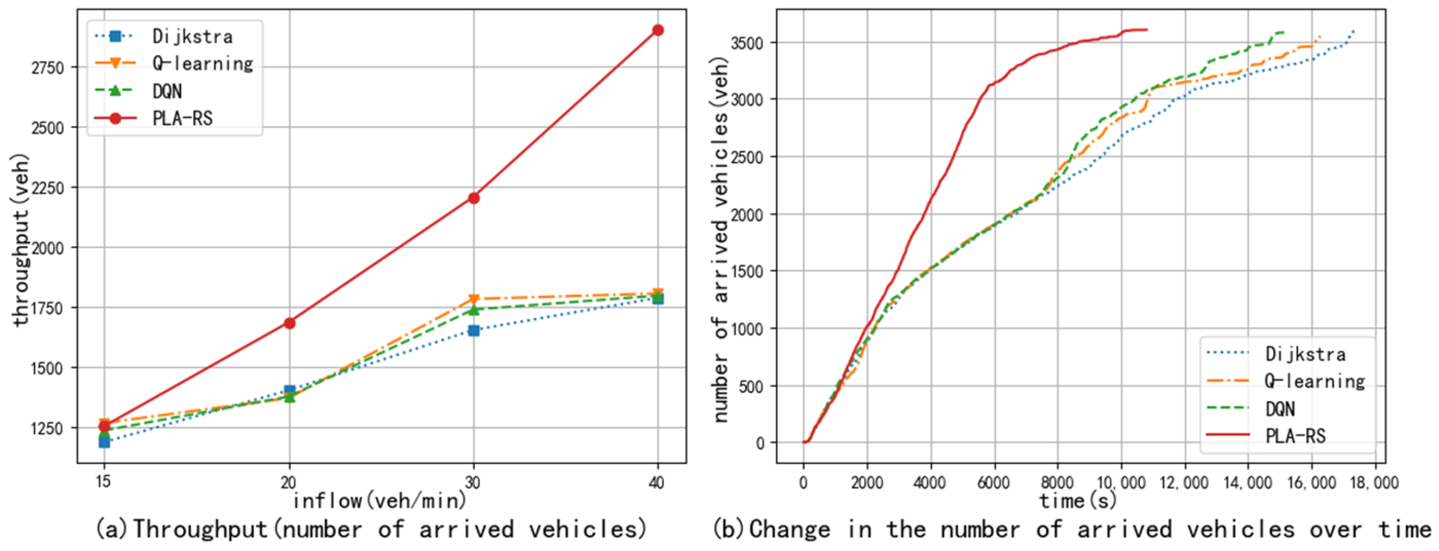
The throughput and the throughput process at maximum traffic flow are shown in Figure 11.
The advantages of the PLA-RS over the artificial road network are illustrated in Figure 11, particularly under the throughput metrics. As traffic flow increases in the more complex real road network, the PLA-RS demonstrates its advantage sooner compared to the artificial road network. Notably, the throughput of the PLA-RS consistently grows as traffic becomes congested, at the same time as the effectiveness of the Q-Learning algorithm and the DQN algorithm diminishes due to the extreme congestion. The Q-Learning algorithm and the DQN algorithm primarily manifest their effects in the middle and late stages of the experiment in terms of the road network’s throughput under congested flow. Conversely, the PLA-RS stands out as the only algorithm capable of maintaining a high decision-making capability during the most severe congestion periods.
The average travel time and average travel cost for different traffic flows are shown in Figure 12.
The experiments on travel time and cost demonstrate that PLA-RS performs better in reducing time and overall travel costs in complex road networks compared to artificial road networks. It also reduces travel costs more effectively at lower traffic flows.
The winners and losers at different traffic flows are shown in Figure 13.
As can be seen from Figure 13, the PLA-RS still shows a slight disadvantage at lower traffic flows and a significant advantage at higher traffic flows. Compared to an artificial road network, the PLA-RS shows a larger gap between the number of winners and losers compared to the Q-Learning algorithm and the DQN algorithm in a more complex real road network.
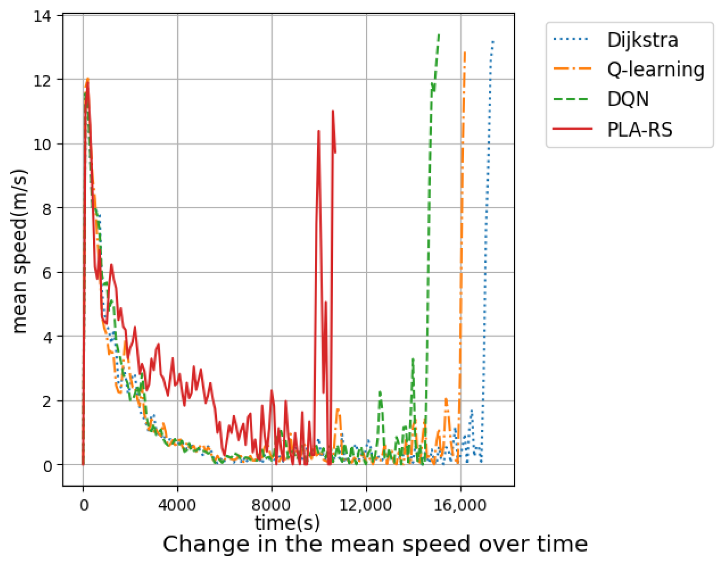
The variation in the average speed of the road network with time under the congested flow is shown in Figure 14.
The experimental results of average speed show that in the real road network the PLA-RS can achieve a wider interval of advantage in time than in the artificial road network. The PLA-RS outperforms the Q-Learning algorithm and the DQN algorithm in a broader timeframe, extending beyond the middle and late stages of the experiments. Specifically, during peak traffic hours from 2000 s to 6000 s, the PLA-RS widens the performance gap with the other algorithms.
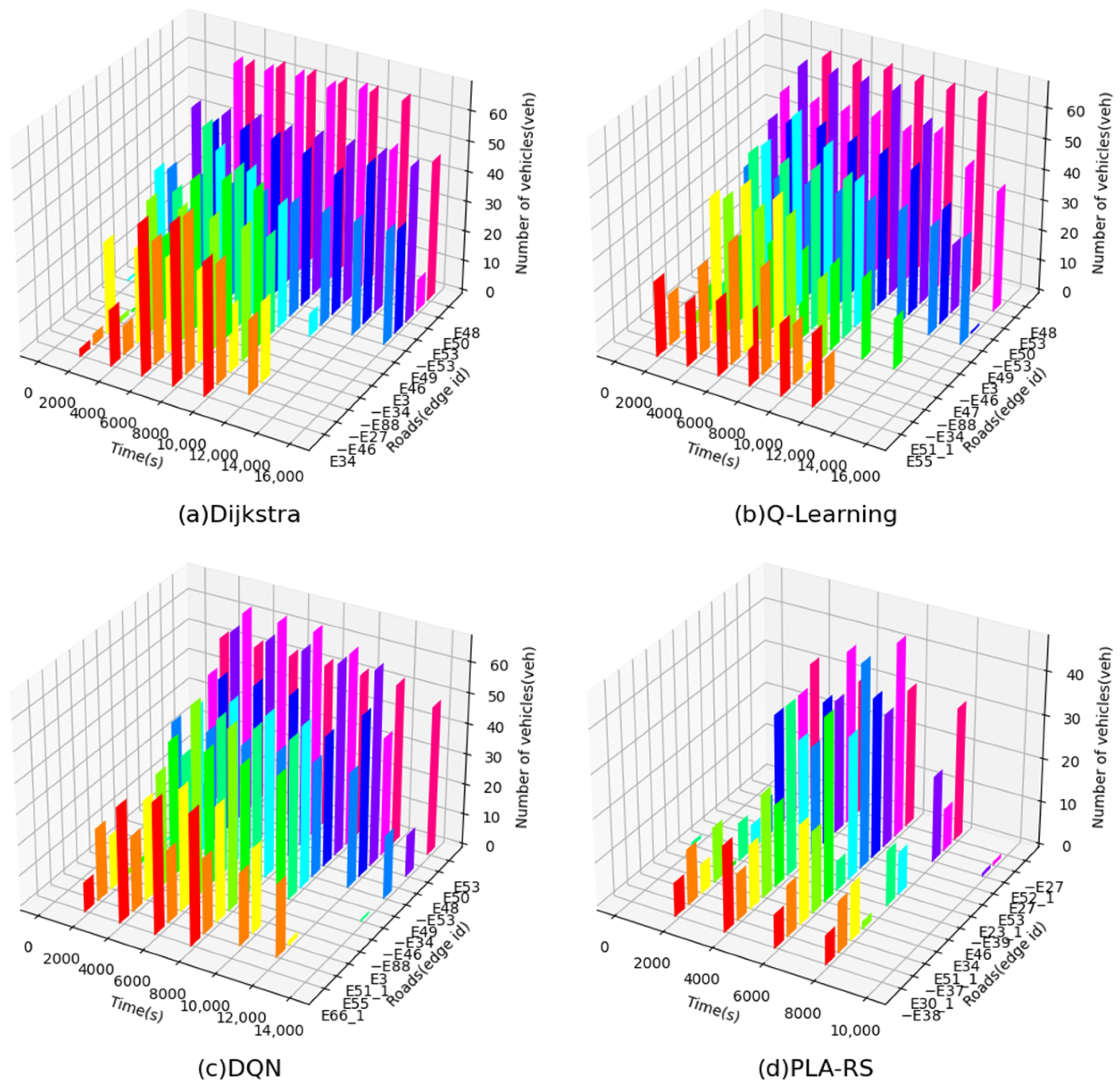
The variation of the numbers of vehicles over time on the 12 roads with the highest numbers of vehicles passing under each algorithm under the congested flow is shown in Figure 15.
Figure 15 shows that the PLA-RS experiences less congestion at the most congested part of the real road network compared to other algorithms. However, the distribution of vehicles is not as uniform as in the artificial road network. Given the greater number of roads on the real road network, it is probable that vehicles are dispersed elsewhere, while under the three non-negotiated algorithms, there is a higher concentration of vehicles. This suggests that the PLA-RS does a more thorough job of dispersing the traffic flow.
From the experimental results of the real road network, it can be seen that the most significant optimization of the PLA-RS for multi-vehicle route decision making lies in the period when the vehicles continue to enter the network. During the peak traffic period, the coordinated route decision-making ability of the DQN and Q-Learning algorithms is more limited, albeit they are able to alleviate traffic congestion to a certain degree. Their main impact is observed in dispersing traffic flow quickly after the end of the traffic peak. However, the PLA-RS is able to make vehicles arrive at their destinations with stable efficiency even during the peak traffic period, which means that the PLA-RS is able to convert the congested flow into free flow to a certain extent.
6. Conclusions
To alleviate the significant congestion problems in urban road networks, this paper presents the construction of a Period-Stage-Round Route Selection Model (PSRRSM) based on a combination of MARL and game theory. Specifically, the proposed PSRRSM enables road agents to utilize the vehicle population game for assisted learning. In addition, a Period Learning Algorithm for Route Selection (PLA-RS) is constructed to enable the agents to participate in routes decision making to varying degrees according to the periods. Consequently, the multi-vehicle route decision making consistently reaches the Nash equilibrium level, ultimately leading to the maximization of traffic congestion relief and reduction of travel costs. Extensive experiments have been conducted in SUMO, utilizing both artificial and real road networks, serves to demonstrate the superiority of the proposed PSRRSM over three non-negotiated algorithms. The PSRRSM exhibits a higher road network throughput efficiency and lower time, distance, fuel, and pollution costs at the macro level, as well as considerable advantages at the micro level from the drivers’ perspective, temporal details, and spatial details.
In spite of the progress in this paper, there is still some work required to be further studied. Firstly, the decision-making process could be considered for different areas within the network and the inter-area route selection strategy to enhance the applicability and effectiveness of the model on a broader scale. Secondly, to improve vehicle–road cooperative decision making, the combination of the model with signalization control can be explored. Thirdly, more vehicle types should be considered, and with the rise of new energy vehicles [37], traffic scenarios should be set up in which conventional, electric, and hybrid energy vehicles coexist, and the composition of the travel cost should be modified accordingly. Finally, the model operation cost, such as equipment deployment and communications, would need to be considered to make the model more optimized.
Author Contributions
Conceptualization and supervision, methodology and writing—original draft, L.Y.; software, validation, formal analysis, visualization, Y.C. All authors have read and agreed to the published version of the manuscript.
Funding
This work is partially supported by National Natural Science Foundation of China (62362031, 62002117); Natural Science Foundation of Jiangxi Province (20224BAB202021).
Data Availability Statement
The datasets analysed during the current study are available in the OpenStreetMap repository, https://www.openstreetmap.org/, accessed on 27 February 2023.
Acknowledgments
The authors also gratefully acknowledge the helpful comments and suggestions of the reviewers, which have improved the presentation.
Conflicts of Interest
The authors declare no conflicts of interest.
Abbreviations
The following abbreviations are used in this manuscript:
| SUMO | Simulation of Urban MObility |
| MARL | Multi-Agent Reinforcement Learning |
| PSRRSM | Period-Stage-Round Route Selection Model |
| PLA-RS | Period Learning Algorithm for Route Selection |
| VMPGA | Vehicle Multi-stage Population Game Algorithm |
References
- Akhtar, M.; Moridpour, S. A review of traffic congestion prediction using artificial intelligence. J. Adv. Transp. 2021, 2021, 8878011. [Google Scholar] [CrossRef]
- Ližbetin, J.; Stopka, O. Proposal of a Roundabout Solution within a Particular Traffic Operation. Open Eng. 2016, 6, 441–445. [Google Scholar] [CrossRef]
- Akcelik, R.; Maher, M. Route control of traffic in urban road networks: Review and principles. Transp. Res. 1977, 11, 15–24. [Google Scholar] [CrossRef]
- Zhu, D.-D.; Sun, J.-Q. A new algorithm based on Dijkstra for vehicle path planning considering intersection attribute. IEEE Access 2021, 9, 19761–19775. [Google Scholar] [CrossRef]
- Liu, Y.; Liu, X. Application of improved A* algorithm in customized bus path planning. Comput. Sci. Appl. 2020, 10, 21–28. [Google Scholar]
- Wang, S.; Lin, F.; Wang, T.; Zhao, Y.; Zang, L.; Deng, Y. Autonomous vehicle path planning based on driver characteristics identification and improved artificial potential field. In Proceedings of the Actuators, Basel, Switzerland, 8 February 2022; p. 52. [Google Scholar]
- Li, Q.; Xu, Y.; Bu, S.; Yang, J. Smart vehicle path planning based on modified PRM algorithm. Sensors 2022, 22, 6581. [Google Scholar] [CrossRef]
- Shi, Y.; Li, Q.; Bu, S.; Yang, J.; Zhu, L. Research on intelligent vehicle path planning based on rapidly-exploring random tree. Math. Probl. Eng. 2020, 2020, 5910503. [Google Scholar] [CrossRef]
- Ahmed, Z.H.; Hameed, A.S.; Mutar, M.L. Hybrid Genetic Algorithms for the Asymmetric Distance-Constrained Vehicle Routing Problem. Math. Probl. Eng. 2022, 2022, 2435002. [Google Scholar] [CrossRef]
- Miao, C.; Chen, G.; Yan, C.; Wu, Y. Path planning optimization of indoor mobile robot based on adaptive ant colony algorithm. Comput. Ind. Eng. 2021, 156, 107230. [Google Scholar] [CrossRef]
- Lu, E.; Xu, L.; Li, Y.; Ma, Z.; Tang, Z.; Luo, C. A novel particle swarm optimization with improved learning strategies and its application to vehicle path planning. Math. Probl. Eng. 2019, 2019, 9367093. [Google Scholar] [CrossRef]
- Li, X.; Zhou, J.; Pedrycz, W. Linking granular computing, big data and decision making: A case study in urban path planning. Soft Comput. 2020, 24, 7435–7450. [Google Scholar] [CrossRef]
- Tang, C.; Hu, W.; Hu, S.; Stettler, M.E. Urban traffic route guidance method with high adaptive learning ability under diverse traffic scenarios. IEEE Trans. Intell. Transp. Syst. 2020, 22, 2956–2968. [Google Scholar] [CrossRef]
- Lu, J.; Li, J.; Yuan, Q.; Chen, B. A multi-vehicle cooperative routing method based on evolutionary game theory. In Proceedings of the 2019 IEEE Intelligent Transportation Systems Conference (ITSC), Auckland, New Zealand, 27–30 October 2019; pp. 987–994. [Google Scholar]
- Ge, Q.; Han, K.; Liu, X. Matching and routing for shared autonomous vehicles in congestible network. Transp. Res. Part Logist. Transp. Rev. 2021, 156, 102513. [Google Scholar] [CrossRef]
- Lowe, R.; Wu, Y.I.; Tamar, A.; Harb, J.; Pieter Abbeel, O.; Mordatch, I. Multi-agent actor-critic for mixed cooperative-competitive environments. In Proceedings of the Advances in Neural Information Processing Systems 30, Long Beach, CA, USA, 4–9 December 2017. [Google Scholar]
- Wang, Z.; Ge, H.; Cheng, R. An extended macro model accounting for the driver’s timid and aggressive attributions and bounded rationality. Physica A 2020, 540, 122988. [Google Scholar] [CrossRef]
- Konda, V.; Tsitsiklis, J. Actor-critic algorithms. In Advances in Neural Information Processing Systems 12; MIT Press: Cambridge, MA, USA, 1999; p. 12. [Google Scholar]
- Misztal, W. The impact of perturbation mechanisms on the operation of the swap heuristic. Arch. Motoryz. 2019, 86, 27–39. [Google Scholar] [CrossRef]
- Šedivý, J.; Čejka, J.; Guchenko, M. Possible application of solver optimization module for solving single-circuit transport problems. LOGI–Sci. J. Transp. Logist. 2020, 11, 78–87. [Google Scholar] [CrossRef]
- Stopka, O. Modelling distribution routes in city logistics by applying operations research methods. Promet 2022, 34, 739–754. [Google Scholar] [CrossRef]
- Paisarnvirosrak, N.; Rungrueang, P. Firefly Algorithm with Tabu Search to Solve the Vehicle Routing Problem with Minimized Fuel Emissions: Case Study of Canned Fruits Transport. LOGI–Sci. J. Transp. Logist. 2023, 14, 263–274. [Google Scholar] [CrossRef]
- Zhang, L.; Khalgui, M.; Li, Z.; Zhang, Y. Fairness concern-based coordinated vehicle route guidance using an asymmetrical congestion game. IET Intell. Transp. Syst. 2022, 16, 1236–1248. [Google Scholar] [CrossRef]
- Banjanovic-Mehmedovic, L.; Halilovic, E.; Bosankic, I.; Kantardzic, M.; Kasapovic, S. Autonomous vehicle-to-vehicle (v2v) decision making in roundabout using game theory. Int. J. Adv. Comput. Sci. Appl. 2016, 7, 292–298. [Google Scholar] [CrossRef]
- Lin, K.; Li, C.; Fortino, G.; Rodrigues, J.J. Vehicle route selection based on game evolution in social internet of vehicles. IEEE Internet Things J. 2018, 5, 2423–2430. [Google Scholar] [CrossRef]
- Tai, T.S.; Yeung, C.H. Adaptive strategies for route selection en-route in transportation networks. Chin. J. Phys. 2022, 77, 712–720. [Google Scholar] [CrossRef]
- Tanimoto, J.; Nakamura, K. Social dilemma structure hidden behind traffic flow with route selection. Physica A 2016, 459, 92–99. [Google Scholar] [CrossRef]
- Zolfpour-Arokhlo, M.; Selamat, A.; Hashim, S.Z.M.; Afkhami, H. Modeling of route planning system based on Q value-based dynamic programming with multi-agent reinforcement learning algorithms. Eng. Appl. Artif. Intell. 2014, 29, 163–177. [Google Scholar] [CrossRef]
- Li, S.; Xu, X.; Zuo, L. Dynamic path planning of a mobile robot with improved Q-learning algorithm. In Proceedings of the 2015 IEEE International Conference on Information and Automation, Lijiang, China, 8–10 August 2015; pp. 409–414. [Google Scholar]
- Liu, S.; Tong, X. Urban transportation path planning based on reinforcement learning. J. Comput. Appl. 2021, 41, 185–190. [Google Scholar]
- Zhou, M.; Jin, J.; Zhang, W.; Qin, Z.; Jiao, Y.; Wang, C.; Wu, G.; Yu, Y.; Ye, J. Multi-agent reinforcement learning for order-dispatching via order-vehicle distribution matching. In Proceedings of the 28th ACM International Conference on Information and Knowledge Management, Beijing, China, 3–7 November 2019; pp. 2645–2653. [Google Scholar]
- Alshehri, M.; Reyes, N.; Barczak, A. Evolving Meta-Level Reasoning with Reinforcement Learning and A* for Coordinated Multi-Agent Path-planning. In Proceedings of the 19th International Conference on Autonomous Agents and MultiAgent Systems, Auckland, New Zealand, 9–13 May 2020; pp. 1744–1746. [Google Scholar]
- Nazari, M.; Oroojlooy, A.; Snyder, L.; Takác, M. Reinforcement learning for solving the vehicle routing problem. In Proceedings of the Advances in Neural Information Processing Systems 31, Montréal, QC, Canada, 3–8 December 2018. [Google Scholar]
- Li, J.; Ma, Y.; Gao, R.; Cao, Z.; Lim, A.; Song, W.; Zhang, J. Deep reinforcement learning for solving the heterogeneous capacitated vehicle routing problem. IEEE Trans. Cybern. 2021, 52, 13572–13585. [Google Scholar] [CrossRef] [PubMed]
- Nai, W.; Yang, Z.; Lin, D.; Li, D.; Xing, Y. A Vehicle Path Planning Algorithm Based on Mixed Policy Gradient Actor-Critic Model with Random Escape Term and Filter Optimization. J. Math. 2022, 2022, 3679145. [Google Scholar] [CrossRef]
- Albaba, B.M.; Yildiz, Y. Driver modeling through deep reinforcement learning and behavioral game theory. IEEE Trans. Control Syst. Technol. 2021, 30, 885–892. [Google Scholar] [CrossRef]
- Li, Z.; Su, S.; Jin, X.; Xia, M.; Chen, Q.; Yamashita, K. Stochastic and distributed optimal energy management of active distribution network with integrated office buildings. CSEE J. Power Energy Syst. 2022, 10, 504–517. [Google Scholar]
Figure 1.
Period-Stage-Round Route Selection Model for urban road network.

Figure 2.
Directed graph for a simple road network.

Figure 3.
Training process of road agents.

Figure 4.
Artificial road network.

Figure 5.
Throughput under different traffic flows and throughput process under congested flow in the artificial road network.
Figure 5.
Throughput under different traffic flows and throughput process under congested flow in the artificial road network.

Figure 6.
Average travel time and average travel cost under different traffic flow in the artificial road network.
Figure 6.
Average travel time and average travel cost under different traffic flow in the artificial road network.

Figure 7.
Winners and losers compared to Dijkstra method for different traffic flows in the artificial road network.
Figure 7.
Winners and losers compared to Dijkstra method for different traffic flows in the artificial road network.

Figure 8.
Change in the average vehicle velocity over time under congested flow in the artificial road network.
Figure 8.
Change in the average vehicle velocity over time under congested flow in the artificial road network.

Figure 9.
Changes in the numbers of vehicles on the 12 most congested roads in the artificial road network.
Figure 9.
Changes in the numbers of vehicles on the 12 most congested roads in the artificial road network.

Figure 10.
Part of the road network in Minhang District, Shanghai.

Figure 11.
Throughput at different traffic flows and throughput process at 40 veh/min in the real road network.
Figure 11.
Throughput at different traffic flows and throughput process at 40 veh/min in the real road network.

Figure 12.
Average travel time and average travel cost for different traffic flows in the real road network.
Figure 12.
Average travel time and average travel cost for different traffic flows in the real road network.

Figure 13.
Winners and losers compared to Dijkstra method for different traffic flows in the real road network.
Figure 13.
Winners and losers compared to Dijkstra method for different traffic flows in the real road network.

Figure 14.
Change in the average vehicle velocity over time under congested flow in the real road network.
Figure 14.
Change in the average vehicle velocity over time under congested flow in the real road network.

Figure 15.
Changes in the numbers of vehicles on the 12 most congested roads in the real road network.
Figure 15.
Changes in the numbers of vehicles on the 12 most congested roads in the real road network.


Table 1.
Definition of parameters of PLA-RS.
| Notation | Instruction | Value |
|---|---|---|
| Time step. | 60 s | |
| Road capacity. | ||
| B | Maximum stage number of the game. | 4 |
| T | Number of rounds per stage. | 100 |
| Exploration probabilities for mixed strategies. | 0.35 | |
| Weights of each of the sub-costs of travel cost. | 0.7599, 0.05, 0.0001, 0.09, 0.1 | |
| Replay buffer capacity. | 3125 | |
| Sample size. | 256 | |
| Period transformation step boundary 1. | 256 | |
| Period transformation step boundary 2. | 3125 | |
| Exploration probability of agents’ choice of actions. | 0.1 | |
| Attenuation factor. | 0.95 | |
| Learning rate (actors). | 0.0001 | |
| Learning rate (critics). | 0.001 |
Disclaimer/Publisher’s Note: The statements, opinions and data contained in all publications are solely those of the individual author(s) and contributor(s) and not of MDPI and/or the editor(s). MDPI and/or the editor(s) disclaim responsibility for any injury to people or property resulting from any ideas, methods, instructions or products referred to in the content. |
© 2024 by the authors. Licensee MDPI, Basel, Switzerland. This article is an open access article distributed under the terms and conditions of the Creative Commons Attribution (CC BY) license (https://creativecommons.org/licenses/by/4.0/).
Share and Cite
MDPI and ACS Style
Yan, L.; Cai, Y. Population Game-Assisted Multi-Agent Reinforcement Learning Method for Dynamic Multi-Vehicle Route Selection. Electronics 2024, 13, 1555. https://doi.org/10.3390/electronics13081555
AMA Style
Yan L, Cai Y. Population Game-Assisted Multi-Agent Reinforcement Learning Method for Dynamic Multi-Vehicle Route Selection. Electronics. 2024; 13(8):1555. https://doi.org/10.3390/electronics13081555
Chicago/Turabian StyleYan, Liping, and Yu Cai. 2024. "Population Game-Assisted Multi-Agent Reinforcement Learning Method for Dynamic Multi-Vehicle Route Selection" Electronics 13, no. 8: 1555. https://doi.org/10.3390/electronics13081555
Note that from the first issue of 2016, this journal uses article numbers instead of page numbers. See further details here.