
Improved Fault Diagnosis of Roller Bearings Using an Equal-Angle Integer-Period Array Convolutional Neural Network

School of Electronic Information Engineering, Xi’an Technological University, Xi’an 710021, China
*
Author to whom correspondence should be addressed.
Electronics 2024, 13(8), 1576; https://doi.org/10.3390/electronics13081576
Submission received: 20 March 2024
/
Revised: 15 April 2024
/
Accepted: 16 April 2024
/
Published: 20 April 2024
Abstract
:This article presents a technique to carry out fault classification using an equal-angle integer-period array convolutional neural network (EAIP-CNN) to process the electrostatic signal of working roller bearings. Firstly, electrostatic signals were collected using uniform angle sampling to ensure the angle intervals between two adjacent data points stayed the same and the signal length was fixed to a pre-determined number of rotation cycles. Then, this one-dimensional signal was transformed into a two-dimensional matrix, where the component of each row was the signal in one period, and the ordinate value of each row represented the corresponding rotation period. Therefore, the row and column indexes of the matrix had a specific meaning instead of simply splitting and stacking the data. Finally, the matrixes were utilized to train the CNN network and test the classification performance. The results show that the classification rate using this technique reaches 95.6%, which is higher than that of 2D CNNs without equal-angle integer-period arrays.
1. Introduction
As the key component used in rotational machinery for power transmission, roller bearings support the rotation of shafts, gears, and drills to improve transmission efficiency. Mostly, the bearings work continuously under heavy loads, high speed, and dusty environments, which makes the bearings prone to damage and causes failure [1]. Statistics show that bearing failure accounts for about 40% of rotating machinery and equipment failure [2,3,4]. If the health condition of roller bearings cannot be detected in a timely manner, further damage may occur and impact the normal operation of related equipment. Therefore, it is of great significance to execute timely and accurate fault diagnosis for roller bearings to avoid further deterioration and operation accidents.
At present, the fault diagnosis methods of roller bearings are mainly divided into two categories: physical model-based methods and data-driven methods [5]. However, model-based methods depend on the accuracy of physical modeling, which is very difficult considering the complicated operating environment in the field and the deviations from ideal simulation conditions. Thus, the application of these methods is limited. Now, data-driven methods have caught researchers’ attention because they can make good use of big data and avoid complicated computation and, probably, the existing errors of physical models [6]. Data-driven methods adopt signal analysis, feature extraction, and dimension reduction to process historical operating data, employ pattern recognition technology to construct comprehensive classification models, and carry out pattern recognition on real-time monitoring data [7,8]. Artificial neural networks (ANNs) [9], support vector machines (SVMs) [10], and cluster analysis (CA) [11] are the commonly used data-driven fault diagnosis models, and are usually combined with adaptive signal processing and effective feature extraction methods.
An ANN is a kind of machine learning model that simulates the brain’s neural structure and information transmission mode. Examples include back propagation (BP) neural networks [12], wavelet neural networks [13], self-organizing feature mapping neural networks [14], and multilayer perception (MLP) neural networks. Satish B et al. [15] proposed a fuzzy BP neural network structure which combines a neural network and fuzzy logic to identify the working state of induction motor bearings and estimate the remaining life of a motor. In [16], an adaptive neuro-fuzzy inference system was utilized as a pattern recognition tool to model multi-scale entropy feature samples extracted from bearing vibration signals. De Almeida et al. [17] use an MLP neural network to train bearing monitoring data from CWRU (Western Reserve University) and RANDALL databases. A recognition rate of 95% can be achieved with fewer input nodes, which verifies the effectiveness of the MLP neural network in bearing fault diagnosis. Khajavi et al. [18] use the standard deviation of the discrete wavelet coefficient as a feature and build a fault classification model based on neural networks.
SVMs, as another commonly used pattern recognition tool, have special advantages when dealing with small sample space, high dimensional features, and nonlinear conditions. In [19], an improved support-vector-machine-based binary tree was proposed to construct multiple classifiers for identifying the states of mild, moderate and severe bearing faults. Soualhi et al. [20] propose heath indicators based on the Hilbert–Huang transform (HHT) to show the degradation of the critical components of bearings, and use an SVM and support vector regression to carry out the classification. Wang et al. [21] used Empirical Mode Decomposition (EMD) combined with an auto-regressive model and singular value decomposition to establish feature space. Then, a hyper-sphere-structured multi-class support machine was constructed to classify bearings with different degradation degrees and fault locations. Experimental results show that the improved SVM can achieve a fault recognition rate of 96%. Kou et al. [22] used improved complete-ensemble EMD to extract the energy entropy of different vibration signals and built an optimized fault diagnosis model using an SVM.
Cluster analysis classifies samples by similarity criteria, has unique advantages in the case of no-fault samples or a small number of fault samples, and is often used in unsupervised fault diagnosis modeling. Considering the gradual change process of bearing fault development and the fuzziness of fault characteristics, many scholars have applied fuzzy logic and cluster analysis to bearing fault diagnosis and achieved good results. Yiakopoulos et al. [23] used K-Means clustering to calculate the correlation distance between two measuring points to describe the strength of their linear relationship, which can be used to classify several bearing states. Jing et al. [24] assume that the feature space of normal bearings forms dense clusters while the feature space of the monitoring signals of fault bearings forms coefficient clusters. On this basis, the density-based clustering algorithm is used to successfully distinguish bearings in five states. Liu et al. [11] utilized grey wolf optimization to achieve the most adequate fractional Gabor spectrum and implemented fault diagnosis by matching the relative order of each cluster with the bearing fault characteristic coefficients.
However, these abovementioned data-driven methods have certain defects. Firstly, signal processing and feature extraction are needed, which are highly dependent on expert knowledge, and different features will greatly affect the final result [25]. Secondly, the shallow level of the network limits the learning ability so that it is difficult to make full use of historical data in the current big data environment [26]. With the development of deep learning algorithms, scholars began to pay attention to establishing an end-to-end fault diagnosis model via deep learning that could directly use the original signal or simple transformed data as the input of the model and build a deeper neural network to make use of the huge monitoring data, thus avoiding the defects mentioned above.
Convolutional neural networks (CNNs), originally designed to process image data, have the characteristics of sparse links and weight sharing, and can establish accurate fault models with fewer network parameters in the case of large input data dimensions [27,28]. Currently, the input of a CNN used for fault diagnosis mainly includes one-dimensional signals or two-dimensional arrays, and 2D-CNNs are more widely used for their flexibility in regard to input formality [29,30,31]. However, there is the problem of how to construct a two-dimensional array from a time-series signal [32]. Wen et al. [33] divided one-dimensional vibration data with the length of M2 into M × M two-dimensional signals as the input layer data of a CNN and verified its effectiveness using the fault dataset of a centrifugal pump and hydraulic pump, respectively. Hoang et al. [34] converted one-dimensional vibration monitoring data into matrix data with equal length and width as the data input of a CNN, used two CNN models to classify the two signals, and fused them at the decision level, so as to realize bearing fault diagnosis. In [35], vibration sensor signals in the X, Y, and Z directions were directly superimposed to construct a matrix as the input of a CNN. Chen et al. [36] extracted 251 features from the sub-band spectrum in the frequency domain and 3 features in the time domain, adding 2 parameters of speed and load, thus forming a total of 256 feature values. Then, these 256 feature values were converted into a 16 × 16 matrix as the CNN input. From the above process of converting one-dimensional data into a two-dimensional matrix, it can be seen that the method of directly splitting and rearranging one-dimensional data lacks longitudinal correlation between the adjacent data segments, making the matrix lack physical meaning. Also, different signal interception lengths will produce different experimental results, which introduces certain human interference factors. Meanwhile, the construction methods above have not considered the rotational properties of roller bearings.
Thus, considering the manual factors brought by the two-dimensional matrix construction methods above, this article proposes a CNN fault diagnosis method combined with uniform angle sampling. Uniform angle sampling techniques are widely used in many industries [37,38], and thus data for order analysis can be easily sourced. Firstly, uniform angle sampling techniques are used to collect data with equal-angle intervals rather than the commonly used sampling method with equal time intervals. Then, the sampled data are divided into several segments, with each corresponding to a rotational cycle. The segments are re-arranged into two-dimensional matrix data, where the row index represents the number of rotation cycles and the column index represents the angular position of the rotation axis. Finally, the matrix with uniform angle and integral cycles is traded as the input of the CNN to build a fault diagnosis mode for roller bearings. The proposed method utilizes the rotational properties of roller bearings to construct a two-dimensional matrix with a certain physical meaning, which can greatly reduce the influence of manual operation. In our method, the input matrix is like a time–space array, where data along the row vary with time and data along the column have the same angle relative to the rising edge of the key signal. Thus, for the whole process of the CNN, the feature maps contain time and space information.
The rest of this paper is organized as follows. Section 2 presents the introductions about the basic theory of convolutional neural networks and the fault diagnosis method based on the equal-angle integer-period array convolutional neural network (EAIP-CNN). Section 3 describes the implementation of uniform angle sampling and the construction of the equal-angle integer-period array and the electrostatic sensor. The fault classification results and analysis are given in Section 4. Section 5 contains the conclusions.
2. Materials and Methods
2.1. Basic Theory of Convolutional Neural Networks
Due to the fact that subsequent processing mainly uses two-dimensional data as input objects, the following explanation will use a 2D-CNN as an example. Convolutional neural networks generally consist of an input layer, convolutional layers, pooling layers, and fully connected layers, where convolutional and pooling layers usually appear in pairs. Additionally, in order to enhance model performance, batch normalization, and activation function, operations are often incorporated in the intermediate processing.
2.1.1. Convolutional Layer
The convolutional layer is an essential component of CNNs. It uses multiple convolutional kernels to perform convolutions on the data from the upper layer, resulting in corresponding feature maps. It has two special advantages: (1) local connectivity, where each convolutional kernel is only connected to a subset of nodes from the previous layer, effectively reducing the number of parameters and accelerating training; and (2) weight sharing, where each convolutional kernel maintains the same weight when moving across the previous layer’s feature map, further reducing the number of parameters. These two characteristics enable CNNs to effectively process high-dimensional data.
By using multiple convolutional kernels, various types of feature information can be obtained. The convolution operation of a single kernel with a single channel is illustrated in Figure 1, where the gray part represents the convolutional kernel. Within the corresponding local receptive field, the specific convolution operation can be expressed as follows:
where represents the value at the position of in the corresponding output feature map. represents the receptive field in the previous layer’s feature map. indicates a convolution operation with a stride of s. represents the convolutional kernel of size k1 × k2 for that layer, and corresponds to the elements within the convolutional kernel. b stands for the bias term. It can be observed from Figure 1 that a convolution operation with a stride of 1 also results in a reduction in the data dimension. In practical applications, it is common to perform zero-padding around the original matrix to ensure that the post-convolution structure maintains the same data dimensions.
As for a multi-channel convolution scenario, assuming the previous layer contains C feature maps of size d1 × d2, where the dimensions of the convolutional kernel are width k1, height k2, and depth C, and the number of kernels is M with a stride of s, the convolution generates M feature maps. The schematic diagram is illustrated in Figure 2, where C = 3, k1 = k2 = 2, and M = 2 for this example. The computation of multi-channel convolution is as follows:
In order to introduce a certain level of nonlinearity into the system to better address complex problems, it is necessary to apply a nonlinear activation function to the data after the convolution operation in the network. The Sigmoid and Tanh functions are the often utilized activation functions in fully connected layers. In comparison to the Sigmoid and Tanh functions, Leaky ReLU and ReLU are more widely applied in CNNs due to their ability to accelerate the learning process and prevent gradient explosion.
2.1.2. Pooling Layer
The pooling layer, also known as the subsampling layer, is primarily responsible for downsampling the feature maps obtained after the convolution operation, following certain rules to reduce data dimensions. Common pooling methods include average pooling, max pooling, and stochastic pooling. These pooling techniques operate on pooling regions within the feature map to reduce redundancy, enhancing the robustness of the post-convolution feature maps.
Typically, convolutional layers and pooling layers are combined within convolutional neural networks (CNNs). In a deep convolutional neural network (DCNN), lower-level convolutional layers extract generalized low-level abstract features from the data, such as edges and contours. On the other hand, higher-level convolutional layers can capture highly abstract features, automating feature extraction and achieving the final classification task.
2.1.3. Fully Connected Layer
After several convolutional and pooling layers, low-dimensional feature information is obtained. This allows for the use of fully connected network nodes, similar to those in a feedforward neural network, to map the feature information to classification labels. The output expression of the fully connected layer is as follows:
where corresponds to the one-dimensional output of the fully connected layer, l represents the number of target classes in the network, denotes an element in the one-dimensional vector obtained by flattening the final feature map, signifies the weights connecting to in a fully connected manner, and is the bias term.
2.1.4. Decision Layer
For classification tasks, the output values of each neuron in the fully connected layer are passed to a classification decision layer that generates an output probability distribution. Currently, the softmax logistic regression function is commonly used for classification, and this layer also can be named as the softmax layer. The computation of the probability output is as follows:
2.2. Fault Diagnosis Method Based on EAIP-CNN
Due to the fact that monitoring signals are predominantly one-dimensional in most cases, a key issue of using a two-dimensional CNN for fault classification is transforming one-dimensional data into a two-dimensional format. From the aforementioned process of converting one-dimensional data into two-dimensional data, it is evident that directly splitting and rearranging one-dimensional data to generate a two-dimensional matrix lacks vertical correlation between the adjacent data segments. Different signal segment lengths can lead to varying experimental results, introducing artificial interference. It is more practical if the elements used for the convolution operation all have the same attributes or physical meaning. Thus, a CNN based on an equal-angle integer-period array method is proposed, as shown in Figure 3.
In Figure 3, the raw signal should be sampled using uniform angle sampling and the data length should be an integral multiple of the length within one cycle. Then, the raw data are divided into several segments of signals with the length of a single cycle. The segments are rearranged according to their sequences of cycles to form the equal-angle integer-period array, which is the data input for the CNN classification model. Within the training process, the loss function is built using the cross-entropy between the already-known target distribution and the estimated softmax output probability from the model, which can be calculated via Equation (5), where p(x) is the target distribution of the training data and q(x) is the estimated distribution output during the training process. In this method, stochastic gradient descent is applied to find the best loss function value and build the final model structure.
2.2.1. Construction of Equal-Angle Integer-Period Array
This 2D matrix construction method requires data series sampled with uniform angles and contains integer rotation cycles. The procedure of the construction method is shown in Figure 4; the newly constructed matrix has the row index representing the number of rotation cycles and the column index representing the angular position of the rotation axis. Therefore, the horizontal coordinate is the angle index and the vertical coordinate is the rotation period index. In Figure 4, matrix row index i represents the rotational period, while column index j represents the angular position relative to the pulse square wave. The relationship between the one-dimensional data and the elements in the two-dimensional matrix is as follows:
2.2.2. Properties of Angle Cycle Array in the Process of CNN
(1) Self-adaptive space filtering. As shown in Equation (6), the convolution operations of the CNN are performed on the data within the rectangular receptive field by a convolution kernel:
Equation (7) is similar to the spatial filtering operation in digital image processing, and the spatial filtering processing of the digital image is shown in the following equation:
By comparing Equations (7) and (8), it can be seen that the convolution operation of the CNN introduces an additional bias term b and step size s, compared with the spatial filtering operation in the image. The spatial filter w in digital image processing is often manually selected; for example, a smooth linear filter is selected for fuzzy processing and noise reduction, and first-order differential Sobel operators and second-order differential Laplacian operators are selected for image sharpening. The convolution kernels in the CNN are obtained by a training process, and the use of the activation function introduces nonlinearity into the system. Therefore, the convolution operation of the CNN can be regarded as a process of adaptive spatial filtering of the original image and adding nonlinearity through the activation function.
Therefore, it is more practical if the elements feeding into the convolution operation have the same physical meaning. When an equal-angle integral-period matrix is used, the convolution kernel of the CNN’s convolution operation covers elements in the receptive field with similar properties; that is, the receptive field elements are signals collected from several adjacent rotation periods within the same rotation angle range. Therefore, the convolution operation of the CNN produces characteristic parameters with certain physical significance.
(2) Feature dimension reduction. The convolution matrix still retains the angle and period information. A pooling operation is needed to facilitate subsequent processing and reduce network complexity. Common pooling methods include maximum pooling and average pooling. Maximum pooling corresponds to the maximum event in the retention feature, that is, the time and amplitude of the maximum feature value in multiple periods. Average pooling can effectively retain the average information of the eigenvalues in the same angle range over multiple rotation cycles. In this paper, maximum pooling is adopted to preserve the peak information of the features.
(3) Properties of feature map.
Finally, our method will transform the original input matrix into several output matrixes, as shown in Figure 5. An individual feature in Figure 5 is processed by the signals from several consecutive rotational cycles within the corresponding angle region. Therefore, each element represents a feature adaptively extracted within the approximate angular interval.
Seen from angular perspective: the row of the output matrix retains the distribution of feature values along the angular direction. Seen from time perspective: features along the column direction represent the distribution across multiple rotational periods within the same angular interval. Seen from scale perspective: the original scale space with an angular resolution of 2π/m and a time resolution of T is transformed to a space with an angular resolution of 2π/m′ and a time resolution of nT/T′.
3. Implementation of Uniform Angle Sampling and Experiment Setup
In practical applications, the uniform angle sampling method is often selected according to the actual situation. Commonly used techniques include encoder-based, computed order tracking, and key-phase signal-based uniform angle sampling.
The encoder-based equal-angle sampling technique utilizes a photoelectric pulse encoder to a specific number of pulse signals in each rotation cycle, which is used as the input to the sampling frequency synthesizer. The frequency synthesizer adjusts the sampling rate and the tracking filter cutoff frequency according to the system sampling order ratio requirements.
Computed order tracking technology first obtains an asynchronous sampling signal by sampling the pulse signal of the tachometer and the sensor signal with equal time intervals. Then, the uniform-angle signals are obtained by interpolating and resampling on the MCU or PC.
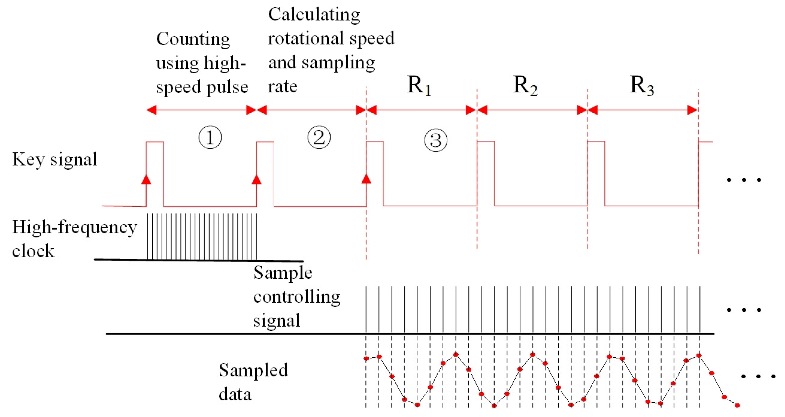
As with key-phase signal-based uniform angle sampling, the reference rotational speed signal is synchronized with the rotation frequency, producing only one square wave pulse within a single rotation cycle. The process is illustrated in Figure 6. Initially, a high-frequency counter is used to count the number of high-frequency clocks between two consecutive key-phase signals. This count is then used to calculate the rotational speed of the shaft. Subsequently, based on the obtained rotational speed and required angular resolution, the sampling frequency needed for subsequent sampling is calculated. Finally, the sampling control signal is employed for signal acquisition at the rising edge of the successive key-phase signal, achieving equal-angle sampling synchronized with the key-phase signal.
Since the experimental section of this paper involves data collection under stable rotational speed conditions, the aforementioned uniform angular sampling based on the key-phase signal is highly suitable for this experiment. In our experiment, the key signal is generated by an electrostatic sensor using the method introduced in reference [39]. In the reference, a PTFE strip is stuck on the rotation shaft and an electrode strip is fixed nearby the PTFE strip. When the shaft rotates, the PTFE strip accumulates charges on its surface and rotates across the electrode with every cycle; thus, the electrode can transform the periodical-induced charges into voltage waveform. Then, a hysteresis voltage comparator circuit is used to transform the periodical voltage waveform into a square wave, which provides the needed key signal. The sampling system used in this article is built based on AD7746, which is the same as that of reference [40]. The system implements uniform angle sampling, as referenced in Figure 6. Firstly, within the square wave ① of the key signal, a counter which starts at the rising edge and stops at the adjacent rising edge is used in the FPGA to count the number of high-frequency clock pulses. Thus, the periodic time of rotation can be obtained and the sampling rate needed for the required angle resolution can also be calculated within the square wave ②. Then, the FPGA chip can generate a sample controlling signal according to the needed sampling rate, which starts the first sampling at the rising edge between square wave ② and ③. The sample controlling signal is directly connected to the SYNC_IN pin on the AD7746 chip, which collects and converts one point of data after every pulse on the SYNC_IN pin.
Experiments are conducted at a rotational speed of 1800 rpm, and the electrostatic monitoring signals are collected using four working conditions of bearings, including normal, outer-race fault, inner-race fault, and rolling element fault. The fault bearings are manually pre-damaged using electrical discharge machining, and the size of the fault area is about 1 mm × 1 mm with a 0.5 mm depth. The detailed signal acquisition parameters are listed in Table 1.
The two-dimensional array images rearranged according to the parameters in Table 1 are shown in Figure 7. It can be seen that the image of the damaged outer ring bearings has obvious distributions of higher energy in the vertical direction. Moreover, the signal images of the inner ring faults and ball faults have obvious pinstripes, while the corresponding image of normal bearings is relatively uniform.
Subsequently, the experimental data are divided into training, validation, and testing sets in certain proportions. The total number of samples is 720, with 480 samples for training, 120 samples for validation, and the last 120 samples for testing, all randomly and evenly extracted from the datasets of every condition. After partitioning the datasets, an appropriate CNN network structure is constructed.
In this paper, a three-layer convolutional neural network (CNN) is employed, as illustrated in Figure 8. The dimensions of the convolutional kernels and the feature maps after pooling operations are displayed in the format [height width channel] in Figure 8. Thus, “16@[9 9 1]” means that there are 16 convolution kernels and the height, width, and channel of each kernel are equal to 9, 9, and 1, correspondingly. The annotation “#1” means the stride of the convolution is equal to 1. “Padding” denotes the zero-padding operation to maintain the dimensions of the resulting matrix consistent with the original matrix. After each convolutional layer, batch normalization and LeakyReLU activation functions are applied for rectification. Finally, the softmax layer is utilized to output the fault diagnosis results.
4. Experiment Results and Analysis
The initial learning rate is set to 0.01, the batch data processing size is set to 80 groups, and the maximum number of training epochs is set to 30 epochs, with each epoch consisting of 480/80 iterations. The maximum number of iterations is set to 180. During the training process, cross-entropy is chosen as the loss function to train the model. Figure 9 displays the accuracy of the training and validation data, as well as the model’s loss function during the training process. The proposed method is implemented by C++ using the MS Visual Studio 2013 in 64-bit.
4.1. Fault Diagnosis Results
Table 2 presents the classification results of the test data with a recognition accuracy of 97.5%. In Table 2, it can be observed that both the normal bearings and inner-race fault bearings are correctly identified, and no other states are recognized as these two states. Among the 30 sets of test data for inner-race fault bearings, 2 sets were identified as ball faults, and among the 30 sets of test data for ball fault bearings, 1 set was identified as an inner-race fault.
In order to observe the adaptive feature extraction capability of the CNN model, after the network training was completed, the distribution of intermediate-layer data was observed using the T-SNE method. The results are shown in Figure 10. The trained CNN architecture was fed with all data, encompassing training, validation, and testing sets, to show the feature extraction process. This process involves computing the intermediate-feature-layer data and subsequently applying t-SNE analysis to obtain a two-dimensional distribution of these feature-layer data. The observations gleaned from Figure 10 are as follows: After the initial convolutional pooling layer, the t-SNE two-dimensional distributions of various states already exhibit noticeable clustering, albeit with a considerable overlap among the four distinct conditions. Subsequent to the second convolutional pooling layer, the demarcation boundaries between these distributions become more pronounced. In the final phase, following the third convolutional pooling operation, the output features of the normal bearings and outer-race faulty bearings are notably distant from the distributions of the other two fault types. Consequently, distinct boundaries emerge among the distributions of the four fault conditions. By examining the t-SNE-based dimensionality reduction and visualization within Figure 10, it can be broadly inferred that instances of misclassification within the test data predominantly arise at the interface between the outer-race faults and ball faults. The high clustering of the testing data in conjunction with similar data types within Figure 10, despite the modeling process relying solely on training and validation data, underscores the model’s commendable generalization capability.
4.2. Process of Adaptive Feature Extraction
In order to see the self-adaptive feature extraction process and the priority of this method, this part lists the feature maps after every convolutional and pooling layer. Figure 11 gives an example of the pseudo-color image after passing through the first convolutional and pooling layer, giving a set of raw data samples as an example. Given the employment of color scaling to visualize the images, the intensity of colors corresponds to the relative magnitudes of the amplitudes within each individual image, but does not reflect the amplitude of the relationships between images. The first convolutional layer comprises 16 convolutional filters, each generating 16 corresponding feature maps after pooling. As discerned from the figure, the feature maps of samples with outer-race damage exhibit notably distinctive dissimilarities when compared to other states.
Based on the data presented in Figure 11, further progression involves subjecting the data to the second convolutional pooling layer, resulting in the outcomes depicted in Figure 12. At this stage, the individual image matrix dimensions are 16 × 32, with alterations in angle and periodic scale, leading to a diminished image resolution in comparison to Figure 11. The insights drawn from the eight feature maps in Figure 12 are as follows:
- (1)
- In T1, T3, and T7, the feature distribution of normal samples appears relatively uniform, sporadically exhibiting substantial feature values, while the localized maxima are notably pronounced in the damaged states.
- (2)
- A quasi-complementary relationship between different states is apparent in images T2 and T5. Normal samples display a higher occurrence of maximal feature values in T2.
- (3)
- The outer-race fault (ORF) feature map reveals prominent vertical stripes, indicating that larger feature values are concentrated around corresponding angular positions.
- (4)
- Ball fault (BF) samples exhibit localized maxima in regions near the left side in T1, T2, T3, T7, and T8. T5 and T6 reveal distinct horizontal stripe patterns.
Figure 13 illustrate the outcomes of the third convolutional pooling operation, as exemplified in Figure 12. The reduction in dimensions is evident through the pronounced mosaic effect within the images, representing the features adaptively extracted by the CNN. As the number of convolutional layers deepens, these features become increasingly abstract, making it challenging for human observation to extract meaningful information. Nevertheless, the t-SNE results depicted in Figure 10 reveal that the final features exhibit high clustering after dimensionality reduction, indicating strong generalization capabilities. This aspect is beneficial for the fully connected layers and decision-making layers of the CNN to effectively discriminate and classify data.
From the above analysis, it can be observed that the CNN’s adaptive feature extraction process involves progressive convolutional pooling layers, leading to a gradual reduction in dimensions and an increasing abstraction of features.
4.3. Comparison Analysis with Different Models
In order to highlight the advantages of equiangular periodic data arrangement, the following comparative experiments were designed for two models.
Comparative CNN Model 1: This model uses equiangular periodic data arrangement. The original 128 cycles are reduced by 8 cycles to obtain a 120 × 256 matrix, resulting in a total of 30,720 data points. The model structure is outlined in Table 3. In the table, [t b l r] signifies zero-padding on the [top bottom left right] positions of the corresponding matrix. In the model, zero-padding is applied only to convolution layers.
Comparative CNN Model 2: This model utilizes the first 30,720 data points from the original one-dimensional data. The total data points match those of Comparative Model 1. These points are divided into 96 segments, and each segment has 320 points of data. Then, concatenated sequentially to form a 96 × 320 matrix. The network parameters for this model are specified as shown in Table 4.
Table 5 presents the fault diagnosis results for the aforementioned models. From the table, it can be observed that the Comparative Model 1, which employs equiangular periodic matrix arrangement, maintains a recognition accuracy similar to the original approach. However, the recognition accuracy of Comparative Model 2, which uses the first 30,720 data points from the original one-dimensional data, is noticeably lower than the original model and Comparative Model 1.
Using t-SNE two-dimensional visualization, the observations of comparative Model 1 and Comparative Model 2 are displayed in Figure 14 and Figure 15, respectively. The images reveal that in the feature layers, after each convolutional pooling, the t-SNE two-dimensional distribution of data from non-equiangular periodic matrix inputs for Model 2 in Figure 15 demonstrates weaker intra-class clustering tendency compared to the results shown in Figure 14. Particularly, following the final convolutional pooling operation, the t-SNE two-dimensional distribution of Comparative Model 2 portrays a distinct intermingling of scatter points for the normal, inner-race damage, and ball damage states, indicating significant overlap, as well as poor overall clustering of the four states. As a result, the fault classification outcomes of Comparative Model 2 are comparatively suboptimal.
From the recognition outcomes and t-SNE visualizations, it is evident that the ACA-CNN based on equiangular periodic arrangement demonstrates a commendable performance in fault classification. As for Model 1, discarding several rotational cycles has an almost negligible impact on classification accuracy, showcasing the model’s robust generalization ability. On the other hand, despite utilizing equiangular sampling for data acquisition, employing a non-equiangular periodic arrangement similar to Comparative Model 2 results in a layout that lacks direct vertical data correlations. The inconsistent angular intervals within the convolution operation lead to a lack of representativeness in the final outcome, thereby causing a notable decline in recognition accuracy. The t-SNE visualization process of Comparative Model 2 underscores the poor intra-class data clustering and substantial feature distribution overlap among different states, suggesting a weaker generalization capacity for this model.
5. Conclusions
This article presented a technique to carry out fault classification using an equal-angle integer-period array convolutional neural network (EAIP-CNN) to process the electrostatic signal of working roller bearings. The proposed method utilized the rotational properties of roller bearings to construct a two-dimensional matrix with certain physical meaning, which can greatly reduce the influence of manual operation. The proposed method reserves the physical properties when the CNN processes data with convolution or pooling. The results show that the classification rate using this technique reaches 95.6%, which is higher than that of 2D CNNs without equal-angle integer-period arrays. This work did not make use of the time–space information carried by the feature maps in the convolutional and fully connected layers, which may contain information on fault area. Future work will be undertaken to employ this proposed method in the fault diagnosis of roller bearings working at variable rotational speeds with different fault sizes to try to find out the relationship between the data of all connected layers and the fault area.
Author Contributions
Conceptualization, writing—original draft, formal analysis, resources, L.L.; writing—review and editing, F.Z. and X.Y.; validation, C.C. All authors have read and agreed to the published version of the manuscript.
Funding
This work was funded by the Key Research and Development Project of Shaanxi Province (2023ZDLNY-61), the National Natural Science Foundation of China (62203345), and the Open Research Project of the State Key Laboratory of Industrial Control Technology, Zhejiang University, China (ICT2022B16).
Data Availability Statement
The data that support the findings of this study are available from the corresponding author upon reasonable request.
Conflicts of Interest
The authors declare no conflicts of interest.
References
- Orlowska-Kowalska, T.; Wolkiewicz, M.; Pietrzak, P.; Skowron, M.; Ewert, P.; Tarchala, G.; Krzysztofiak, M.; Kowalski, C.T. Fault Diagnosis and Fault-Tolerant Control of PMSM Drives-State of the Art and Future Challenges. IEEE Access 2022, 10, 59979–60024. [Google Scholar] [CrossRef]
- Attoui, I.; Fergani, N.; Boutasseta, N.; Oudjani, B.; Deliou, A. A new time-frequency method for identification and classification of ball bearing faults. J. Sound Vib. 2017, 397, 241–265. [Google Scholar] [CrossRef]
- Burda, E.A.; Zusman, G.V.; Kudryavtseva, I.S.; Naumenko, A.P. An Overview of Vibration Analysis Techniques for the Fault Diagnostics of Rolling Bearings in Machinery. Shock. Vib. 2022, 2022, 6136231. [Google Scholar] [CrossRef]
- Cui, L.L.; Jin, Z.; Huang, J.F.; Wang, H.Q. Fault Severity Classification and Size Estimation for Ball Bearings Based on Vibration Mechanism. IEEE Access 2019, 7, 56107–56116. [Google Scholar] [CrossRef]
- Heng, A.; Zhang, S.; Tan, A.C.C.; Mathew, J. Rotating machinery prognostics: State of the art, challenges and opportunities. Mech. Syst. Signal Process. 2009, 23, 724–739. [Google Scholar] [CrossRef]
- Hou, J.J.; Lu, X.K.; Zhong, Y.D.; He, W.B.; Zhao, D.F.; Zhou, F. A comprehensive review of mechanical fault diagnosis methods based on convolutional neural network. J. Vibroeng. 2024, 26, 44–65. [Google Scholar] [CrossRef]
- Patil, M.S.; Mathew, J.; RajendraKumar, P.K. Bearing signature analysis as a medium for fault detection: A review. J. Tribol. 2008, 130, 014001. [Google Scholar] [CrossRef]
- Yin, S.; Ding, S.X.; Xie, X.C.; Luo, H. A Review on Basic Data-Driven Approaches for Industrial Process Monitoring. IEEE Trans. Ind. Electron. 2014, 61, 6418–6428. [Google Scholar] [CrossRef]
- Farooq, U.; Ademola, M.; Shaalan, A. Comparative Analysis of Machine Learning Models for Predictive Maintenance of Ball Bearing Systems. Electronics 2024, 13, 438. [Google Scholar] [CrossRef]
- Ao, H.; Cheng, J.S.; Yang, Y.; Truong, T.K. The support vector machine parameter optimization method based on artificial chemical reaction optimization algorithm and its application to roller bearing fault diagnosis. J. Vib. Control 2015, 21, 2434–2445. [Google Scholar] [CrossRef]
- Liu, F.; Shang, Z.W.; Gao, M.S.; Li, W.X.; Pan, C.L. Bearing failure diagnosis at time-varying speed based on adaptive clustered fractional Gabor transform. Meas. Sci. Technol. 2023, 34, 095002. [Google Scholar] [CrossRef]
- Jiao, R.; Li, S.; Ding, Z.X.; Yang, L.; Wang, G. Fault diagnosis of rolling bearing based on BP neural network with fractional order gradient descent. J. Vib. Control 2023. [Google Scholar] [CrossRef]
- Lei, Y.G.; He, Z.J.; Zi, Y.Y. Application of an intelligent classification method to mechanical fault diagnosis. Expert Syst. Appl. 2009, 36, 9941–9948. [Google Scholar] [CrossRef]
- Merainani, B.; Rahmoune, C.; Benazzouz, D.; Ould-Bouamama, B. A novel gearbox fault feature extraction and classification using Hilbert empirical wavelet transform, singular value decomposition, and SOM neural network. J. Vib. Control 2018, 24, 2512–2531. [Google Scholar] [CrossRef]
- Satish, B.; Sarma, N.D.R. A fuzzy BP approach for diagnosis and prognosis of bearing faults in induction motors. In Proceedings of the IEEE Power Engineering Society General Meeting, San Francisco, CA, USA, 12–16 June 2005; Volume 2293, pp. 2291–2294. [Google Scholar]
- Zhang, L.; Xiong, G.L.; Liu, H.S.; Zou, H.J.; Guo, W.Z. Bearing fault diagnosis using multi-scale entropy and adaptive neuro-fuzzy inference. Expert Syst. Appl. 2010, 37, 6077–6085. [Google Scholar] [CrossRef]
- de Almeida, L.F.; Bizarria, J.W.P.; Bizarria, F.C.P.; Mathias, M.H. Condition-based monitoring system for rolling element bearing using a generic multi-layer perceptron. J. Vib. Control 2015, 21, 3456–3464. [Google Scholar] [CrossRef]
- Khajavi, M.N.; Keshtan, M.N. Intelligent fault classification of rolling bearings using neural network and discrete wavelet transform. J. Vibroeng. 2014, 16, 761–769. [Google Scholar]
- Li, Y.B.; Xu, M.Q.; Wang, R.X.; Huang, W.H. A fault diagnosis scheme for rolling bearing based on local mean decomposition and improved multiscale fuzzy entropy. J. Sound Vib. 2016, 360, 277–299. [Google Scholar] [CrossRef]
- Soualhi, A.; Medjaher, K.; Zerhouni, N. Bearing Health Monitoring Based on Hilbert–Huang Transform, Support Vector Machine, and Regression. IEEE Trans. Instrum. Meas. 2015, 64, 52–62. [Google Scholar] [CrossRef]
- Wang, Y.J.; Kang, S.Q.; Jiang, Y.C.; Yang, G.X.; Song, L.X.; Mikulovich, V.I. Classification of fault location and the degree of performance degradation of a rolling bearing based on an improved hyper-sphere-structured multi-class support vector machine. Mech. Syst. Signal Process. 2012, 29, 404–414. [Google Scholar] [CrossRef]
- Kou, Z.M.; Yang, F.; Wu, J.; Li, T.Y. Application of ICEEMDAN Energy Entropy and AFSA-SVM for Fault Diagnosis of Hoist Sheave Bearing. Entropy 2020, 22, 1347. [Google Scholar] [CrossRef]
- Yiakopoulos, C.T.; Gryllias, K.C.; Antoniadis, I.A. Rolling element bearing fault detection in industrial environments based on a-means clustering approach. Expert Syst. Appl. 2011, 38, 2888–2911. [Google Scholar] [CrossRef]
- Jing, T.; Azarian, M.H.; Pecht, M. Rolling element bearing fault detection using density-based clustering. In Proceedings of the 2014 International Conference on Prognostics and Health Management, Spokane, WA, USA, 22–25 June 2014; pp. 1–7. [Google Scholar]
- Bengio, Y.; Courville, A.; Vincent, P. Representation Learning: A Review and New Perspectives. IEEE Trans. Pattern Anal. 2013, 35, 1798–1828. [Google Scholar] [CrossRef] [PubMed]
- Zhao, R.; Yan, R.Q.; Chen, Z.H.; Mao, K.Z.; Wang, P.; Gao, R.X. Deep learning and its applications to machine health monitoring. Mech. Syst. Signal Process. 2019, 115, 213–237. [Google Scholar] [CrossRef]
- Jing, L.Y.; Zhao, M.; Li, P.; Xu, X.Q. A convolutional neural network based feature learning and fault diagnosis method for the condition monitoring of gearbox. Measurement 2017, 111, 1–10. [Google Scholar] [CrossRef]
- Luczak, D. Machine Fault Diagnosis through Vibration Analysis: Continuous Wavelet Transform with Complex Morlet Wavelet and Time-Frequency RGB Image Recognition via Convolutional Neural Network. Electronics 2024, 13, 452. [Google Scholar] [CrossRef]
- Shao, H.D.; Jiang, H.K.; Zhang, H.Z.; Duan, W.J.; Liang, T.C.; Wu, S.P. Rolling bearing fault feature learning using improved convolutional deep belief network with compressed sensing. Mech. Syst. Signal Process. 2018, 100, 743–765. [Google Scholar] [CrossRef]
- Shao, H.D.; Jiang, H.K.; Zhang, H.Z.; Liang, T.C. Electric Locomotive Bearing Fault Diagnosis Using a Novel Convolutional Deep Belief Network. IEEE Trans. Ind. Electron. 2018, 65, 2727–2736. [Google Scholar] [CrossRef]
- Wang, F.; Jiang, H.G.; Shao, H.D.; Duan, W.J.; Wu, S.P. An adaptive deep convolutional neural network for rolling bearing fault diagnosis. Meas. Sci. Technol. 2017, 28, 095005. [Google Scholar] [CrossRef]
- Jiao, J.; Zhao, M.; Lin, J.; Liang, K. A comprehensive review on convolutional neural network in machine fault diagnosis. Neurocomputing 2020, 417, 36–63. [Google Scholar] [CrossRef]
- Wen, L.; Li, X.Y.; Gao, L.; Zhang, Y.Y. A New Convolutional Neural Network-Based Data-Driven Fault Diagnosis Method. IEEE Trans. Ind. Electron. 2018, 65, 5990–5998. [Google Scholar] [CrossRef]
- Hoang, D.T.; Kang, H.J. A Motor Current Signal-Based Bearing Fault Diagnosis Using Deep Learning and Information Fusion. IEEE Trans. Instrum. Meas. 2020, 69, 3325–3333. [Google Scholar] [CrossRef]
- Wang, H.Q.; Li, S.; Song, L.Y.; Cui, L.L. A novel convolutional neural network based fault recognition method via image fusion of multi-vibration-signals. Comput. Ind. 2019, 105, 182–190. [Google Scholar] [CrossRef]
- Chen, Z.Q.; Li, C.; Sanchez, R.V. Gearbox Fault Identification and Classification with Convolutional Neural Networks. Shock. Vib. 2015, 2015, 390134. [Google Scholar] [CrossRef]
- Bahmani, M.H.; Esmaeili Shayan, M.; Fioriti, D. Assessing electric vehicles behavior in power networks: A non-stationary discrete Markov chain approach. Electr. Power Syst. Res. 2024, 229, 110106. [Google Scholar] [CrossRef]
- Shayan, M.E.; Najafi, G.; Ghobadian, B.; Gorjian, S.; Mamat, R.; Ghazali, M.F. Multi-microgrid optimization and energy management under boost voltage converter with Markov prediction chain and dynamic decision algorithm. Renew. Energy 2022, 201, 179–189. [Google Scholar] [CrossRef]
- Li, L.; Hu, H.L.; Qin, Y.; Tang, K.H. Digital Approach to Rotational Speed Measurement Using an Electrostatic Sensor. Sensors 2019, 19, 2540. [Google Scholar] [CrossRef]
- Li, L.; Hu, H.; Tang, K. A specially-designed electrostatic sensor for the condition monitoring of rolling bearings. Meas. Sci. Technol. 2021, 32, 035110. [Google Scholar] [CrossRef]
Figure 1.
Illustration of convolution operation.

Figure 2.
Illustration of multi-channel convolution operation.

Figure 3.
Program of fault diagnosis using CNN and uniform angle sampling.

Figure 4.
Transformation of uniform-angle sampled data into an equal-angle integer-period array.

Figure 5.
Properties of CNN feature layer.

Figure 6.
Uniform angle sampling using key signal.

Figure 7.
Equal-angle integer-period arrays of electrostatic signals under different conditions.

Figure 8.
CNN network architecture.

Figure 9.
The accuracy and loss functions of training and validation processes.

Figure 10.
Data visualization of different steps using TSNE.

Figure 11.
Feature data after the first convolution layer.

Figure 12.
Feature data after the second convolution layer.

Figure 13.
Feature data after the third convolution layer.

Figure 14.
Dimension reduction and visualization results using TSNE for Model 1.

Figure 15.
Dimension reduction and visualization results using TSNE for Model 2.


Table 1.
Signal acquisition parameters of each bearing condition.
| Parameter | Rotational Speed/rpm | Number of Sampling Points within One Cycle | Number of Cycles for Sampling | Number of Datasets |
|---|---|---|---|---|
| value | 1800 | 256 | 128 | 180 |
Table 2.
Fault diagnosis results of CNN using equal-angle integer-period array.
| Classification Results | Recall Rate/% | ||||
|---|---|---|---|---|---|
| NR | ORF | IRF | BF | ||
| 30 sets of NR data | 30 | 0 | 0 | 0 | 100 |
| 30 sets of ORF data | 0 | 30 | 0 | 0 | 100 |
| 30 sets of IRF data | 0 | 0 | 28 | 2 | 93.33 |
| 30 sets of BF data | 0 | 0 | 1 | 29 | 96.67 |
| Accuracy Pi% | 100 | 100 | 96.55 | 93.55 | A = 97.5% |
Table 3.
Network construction of Model 1 for comparison.
| Layer | Operation | Zero Fill | Step Length | Output Data Dimension |
|---|---|---|---|---|
| Input | / | / | / | [120 256 1] |
| Convolution 1 | 16@[9 9 1] | [4 4 4 4] | 1 | [120 256 16] |
| Pooling 1 | Max pooling 4 × 4 | [0 0 0 0] | 4 | [30 64 16] |
| Convolution 2 | 8@[5 5 16] | [2 2 2 2] | 1 | [30 64 8] |
| Pooling 2 | Max pooling 2 × 2 | [0 0 0 0] | 2 | [15 32 8] |
| Convolution 3 | 4@[3 3 8] | [1 1 1 1] | 1 | [15 32 4] |
| Pooling 3 | Max pooling 2 × 2 | [0 0 0 0] | 2 | [7 16 4] |
| Full connection | / | / | / | 448 |
Table 4.
Network construction of Model 2 for comparison.
| Layer | Operation | Zero Fill | Step Length | Output Data Dimension |
|---|---|---|---|---|
| Input | / | / | / | [96 320 1] |
| Convolution 1 | 16@[9 9 1] | [4 4 4 4] | 1 | [96 320 16] |
| Pooling 1 | Max pooling 4 × 4 | [0 0 0 0] | 4 | [24 80 16] |
| Convolution 2 | 8@[5 5 16] | [2 2 2 2] | 1 | [24 80 8] |
| Pooling 2 | Max pooling 2 × 2 | [0 0 0 0] | 2 | [12 40 8] |
| Convolution 3 | 4@[3 3 8] | [1 1 1 1] | 1 | [12 40 4] |
| Pooling 3 | Max pooling 2 × 2 | [0 0 0 0] | 2 | [6 20 4] |
| Full connection | / | / | / | 480 |
Table 5.
Classification accuracy of the three models.
| Model | Data Input Dimension | Accuracy/% |
|---|---|---|
| ACA-CNN | Equal-angle integer-period array 128 × 256 | 97.5 |
| ACA-CNN for comparison | Equal-angle integer-period array 120 × 256 | 95.0 |
| CNN | Normal permutation 96 × 320 | 87.5 |
Disclaimer/Publisher’s Note: The statements, opinions and data contained in all publications are solely those of the individual author(s) and contributor(s) and not of MDPI and/or the editor(s). MDPI and/or the editor(s) disclaim responsibility for any injury to people or property resulting from any ideas, methods, instructions or products referred to in the content. |
© 2024 by the authors. Licensee MDPI, Basel, Switzerland. This article is an open access article distributed under the terms and conditions of the Creative Commons Attribution (CC BY) license (https://creativecommons.org/licenses/by/4.0/).
Share and Cite
MDPI and ACS Style
Li, L.; Yuan, X.; Zhang, F.; Chen, C. Improved Fault Diagnosis of Roller Bearings Using an Equal-Angle Integer-Period Array Convolutional Neural Network. Electronics 2024, 13, 1576. https://doi.org/10.3390/electronics13081576
AMA Style
Li L, Yuan X, Zhang F, Chen C. Improved Fault Diagnosis of Roller Bearings Using an Equal-Angle Integer-Period Array Convolutional Neural Network. Electronics. 2024; 13(8):1576. https://doi.org/10.3390/electronics13081576
Chicago/Turabian StyleLi, Lin, Xiaoxi Yuan, Feng Zhang, and Chaobo Chen. 2024. "Improved Fault Diagnosis of Roller Bearings Using an Equal-Angle Integer-Period Array Convolutional Neural Network" Electronics 13, no. 8: 1576. https://doi.org/10.3390/electronics13081576
Note that from the first issue of 2016, this journal uses article numbers instead of page numbers. See further details here.