
Spatial–Temporal Fusion Gated Transformer Network (STFGTN) for Traffic Flow Prediction

1
School of Computer Science and Technology, Shandong University of Technology, Zibo 255000, China
2
Inspur (Jinan) Data Technology Co., Ltd., Jinan 250101, China
*
Author to whom correspondence should be addressed.
Electronics 2024, 13(8), 1594; https://doi.org/10.3390/electronics13081594
Submission received: 25 March 2024
/
Revised: 17 April 2024
/
Accepted: 18 April 2024
/
Published: 22 April 2024
(This article belongs to the Special Issue Applications of Deep Neural Network for Smart City)
Abstract
:Traffic flow prediction is essential for smart city management and planning, aiding in optimizing traffic scheduling and improving overall traffic conditions. However, due to the correlation and heterogeneity of traffic data, effectively integrating the captured temporal and spatial features remains a significant challenge. This paper proposes a model spatial–temporal fusion gated transformer network (STFGTN), which is based on an attention mechanism that integrates temporal and spatial features. This paper proposes an attention mechanism-based model to address these issues and model complex spatial–temporal dependencies in road networks. The self-attention mechanism enables the model to achieve long-term dependency modeling and global representation of time series data. Regarding temporal features, we incorporate a time embedding layer and a time transformer to learn temporal dependencies. This capability contributes to a more comprehensive and accurate understanding of spatial–temporal dynamic patterns throughout the entire time series. As for spatial features, we utilize DGCN and spatial transformers to capture both global and local spatial dependencies, respectively. Additionally, we propose two fusion gate mechanisms to effectively accommodate to the complex correlation and heterogeneity of spatial–temporal information, resulting in a more accurate reflection of the actual traffic flow. Our experiments on three real-world datasets illustrate the superior performance of our approach.
1. Introduction
Intelligent transportation systems (ITS) [1] are integral to the development of smart cities. Within ITS, traffic flow prediction [2] plays a crucial role by accurately forecasting future traffic conditions based on historical observations. Studies have demonstrated that precise traffic flow prediction is essential for tasks such as alleviating congestion and forecasting taxi demand [3] In the transportation domain, “demand” typically refers to the travel or transportation needs of people or goods between different locations. This encompasses factors like the quantity of trips or the volume of goods transported from one location to another. Short-term origin–destination (OD) flow prediction [4,5] is particularly significant for urban rail transit operation planning, control, and freight transport management.
The typical spatial and temporal characteristics observed in traffic flow prediction data pertain to the variations in data across time and location. This trait underscores the prevalence of correlation and heterogeneity within traffic flow data. Correlation primarily entails autocorrelation across both temporal and spatial dimensions. For instance, as depicted in Figure 1, a traffic incident occurring at a specific road node may have a prolonged impact on adjacent road segments’ traffic flow, persisting over multiple time intervals. Heterogeneity, conversely, is evidenced by diverse patterns observed at different temporal or spatial scales. For example, certain holidays or highly trafficked areas may exhibit distinct traffic flow features. So, the primary challenge in predicting traffic flow is effectively capturing and modeling the complex and dynamic correlation and heterogeneity of traffic data. Traditional methods, such as support vector regression (SVR) [6], Bayesian methods [6,7], and vector autoregressive models [8], often rely on complex feature engineering and have poor generalization capabilities.
In recent years, the field of traffic flow prediction has seen widespread use of hybrid neural networks based on convolutional neural networks (CNNs) and recurrent neural networks (RNNs) [8,9,10,11,12] due to the development of deep learning techniques. Examples of such networks include ConvLSTM [13] and PredRNN [14]. However, these methods have a limitation in that they cannot directly address non-Euclidean data inherent in urban systems, such as vehicle flows on road networks. Graph neural networks have rapidly developed to fill the gap in traffic flow prediction. For complex spatial–temporal dependencies, some approaches take into account the existence of multiple spatial relationships by constructing multiple graphs, such as STMGCN [15] and STFGNN [16]. Graph WaveNet [17] utilizes adaptive graph learning to learn spatial dependencies. Regarding temporal dependencies, there are various approaches, including TCNs that use receptive fields of different sizes, such as MTGNN [18]. There are also approaches that capture spatial–temporal dependencies by integrating different learning networks, such as ASTGCN [19]. Additionally, spatial–temporal synchronization graphs can be constructed to establish unified spatial–temporal dependencies between time.
But this adjacency matrix is based on road adjacency or time series similarity and only takes into account the static spatial dependence between roads. However, spatial relationships on real roads undergo dynamic changes influenced by factors such as weather conditions, holidays, and emergencies. Capturing this dynamic change is difficult with a single temporal or spatial module. Furthermore, spatial–temporal relationships in traffic flow tasks are often complex and diverse, involving multiple patterns at different time scales and spatial locations. To accurately and comprehensively fuse this complex information, it is crucial to design model structures that can adapt to different modes and dynamic changes. Consequently, enhancing the accuracy and robustness of traffic flow prediction hinges on the model’s adeptness at effectively fusing spatial–temporal information.
Compared to previous traffic flow prediction models based on encoder–decoder transformer architectures, STFGTN has made the following improvements:
- We introduce a novel spatial–temporal dependency fusion model (STFGTN) for traffic flow prediction, leveraging an attention mechanism. This model effectively captures spatial–temporal correlations, aggregates relevant information, and notably enhances traffic flow prediction accuracy.
- A novel dynamic graph convolutional neural network (DGCN) is employed to capture evolving spatial dependencies among traffic flow data nodes, complemented by an attention mechanism. This network adeptly mines spatial data correlations by dynamically adjusting node correlation coefficients and aggregating high-node-correlation information.
- Two gating mechanisms are incorporated to integrate various components within our model. Firstly, we fuse local spatial features from DGCNs with global spatial features from spatial multi-attention. Secondly, we introduce a gating nonlinearity to fuse previously integrated spatial features with temporal features obtained through temporal multi-head attention.
2. Relation Work
2.1. Deep Learning for Traffic Prediction
In recent years, there has been a surge in the development of deep learning frameworks aimed at addressing traffic flow prediction challenges, with the primary goal of enhancing prediction accuracy. Initially, spatial regions were divided into two or three-dimensional grids, serving as input windows for convolutional neural networks to forecast traffic flow. ST-ResNet [9] utilized residual convolution techniques for crowd flow prediction. Yao et al. [12] employed convolutional neural networks (CNNs) in the spatial domain and long short-term memory (LSTM) in the temporal domain to capture spatial–temporal dependencies in traffic flow data. These methods operate on gridded traffic data and apply convolution operations in a structured manner with respect to spatial dimensions to capture spatial correlations. However, they do not account for non-Euclidean dependencies between nodes.
Graph neural networks (GNNs) have showcased remarkable performance in modeling graph data, rendering them a favored choice for various graph-related tasks like graph classification [20], node classification [21], and recommender systems [22]. Recent studies have integrated spatial graphs into traffic prediction by employing spatial–temporal graph models to handle the graph structure of spatial–temporal data. This approach has been explored by numerous researchers [18,23,24,25,26,27]. The traffic data is organized as a graph using a spatial–temporal graph neural network (STGNN) and utilized for prediction. The STGNN model is divided into two methods: RNN-based and CNN-based. RNNs and CNNs are utilized in the respective methods to conduct forward computation along the temporal dimension. Attentional mechanisms have gained popularity in this domain due to their efficacy in capturing dynamic dependencies in traffic data [19,28,29,30,31]. However, these models do not comprehensively address the dynamic spatial–temporal dependencies between nodes within the road network, at both local and global scales.
Additionally, deep learning techniques aid in origin–destination (OD) estimation for traffic flow prediction [32], using deep learning methods and global sensitivity analysis to solve OD estimation and sensor location issues.
2.2. Graph Convolution Networks
Graph convolutional neural networks (GCNs) are powerful tools for capturing spatial dependencies in non-Euclidean spaces. The crux of GCNs lies in the adjacency matrix, which provides inherent topological information to the model. However, real-world traffic dynamics can vary significantly, even among locations with the same central point, due to factors such as temporal variations. Therefore, the static adjacency matrix constructed by GCNs fails to accurately capture the dynamic nature of traffic diffusion. In recent years, popular GCNs can be classified into three main types: spectral GCN [33,34], ChebNet [35], and GAT [36]. With regard to spectral GCN, Bruna et al. used Fourier transform to convert graph signals in the spatial domain to the spectral domain for convolution computations. In terms of ChebNet, to overcome the dependence on the graph Laplace matrix, Kipf et al. performed message passing in the spatial domain to simplify the graph convolution operation. In terms of GAT, to illustrate the importance of neighboring nodes in learning spatial dependencies, GAT integrates an attention mechanism into the node aggregation operation.
2.3. Transformer
The concept of the attention mechanism aims to enhance model performance by efficiently assigning weights and focusing on different parts of the information, thus making it more adaptable to various tasks and data contexts. This concept has been successfully applied in several deep learning models, including the Transformer architecture in natural language processing [37], and the Swin Transformer in computer vision [38], which achieved remarkable image classification performance. Additionally, numerous variants of the Transformer have demonstrated promising results in computer vision tasks.
Recent studies have shown that introducing the Transformer architecture to traffic flow prediction [27,30,39] addresses the limitations of static structures. The original Transformer architecture employs an encoder–decoder structure, utilizing encoder and decoder stacks to extract deep features, along with a multi-head mechanism to capture long-term dependencies in sequences. For example, in TFormer [40], the K-hop adjacency matrix is used to guide the model to focus on the nearby neighboring nodes and ignore the distant nodes. It describes the adjacency between nodes in the graph and helps the model to accurately capture local spatial features. Traffic Transformer [41] consists of a global encoder and a global–local decoder, integrating global and local spatial features through multi-head attention. It utilizes temporal embedding blocks to extract temporal features, positional encoding and embedding blocks to understand node locations, and concludes with a linear layer for prediction. In our approach, we leverage the Transformer solely as a spatial–temporal dependency extractor, deviating from the original Transformer’s encoder–decoder structure.
3. Problem Definition
Definition 1.
(Road network) We denote the road network as , where denotes the set of N nodes in the road network, E is the set of connectivity between nodes, and is the adjacency matrix of the road network used to describe the spatial distance between nodes. Where N is denoted as the number of nodes in the road network.
Definition 2.
(Traffic Signal Matrix) Therefore, the traffic state at any time step t can be regarded as a graph signal , where D is the dimension of the traffic state, and the state includes traffic flow, speed, etc. We use to denote the traffic flow tensor of all nodes on the total T time step.
Problem Formalization
Traffic flow prediction is the prediction of traffic flow in a future time period by analyzing the observed historical traffic data. In a transportation system, we have observed traffic flow data , and a known spatial graph . Our objective is to learn the mapping function f from the observed historical traffic flow at the T-steps, in order to predict the traffic flow at the future steps.
4. Methods
Figure 2 illustrates the architecture of STFGTNs, comprising a data embedding layer, multiple stacked spatial–temporal modules interconnected in sequence, and an output layer. We will provide a detailed description of each module below.
4.1. Data Embedding Layer
In this study, we introduce an input embedding, a widely employed and effective technical approach. The data embedding layer’s main task is to transform input data into a high-dimensional representation. Specifically, it first transforms the original input into which is a vector in a higher dimensional space through a fully connected layer.
where is the dimension of the embedding, is the traffic series in the previous T time timestamp, and the indicates a fully connected layer.
In order to better model the periodicity of traffic flow, we specifically design an embedding mechanism which can effectively incorporate the time-periodicity information into the model. The urban traffic flow is highly periodic as influenced by people’s traveling mode and lifestyle. For the time periodicity information, we introduce two embeddings to represent the weekly and daily periodicity, respectively, denoted as and , where is the number of days in a week and is the number of timestamp in a day. and denote the day of the week data and, for traffic flow sequences, the timestamped data, respectively. We extract the corresponding temporal embeddings and by using them as indexes. The periodicity embedding for the traffic time series is obtained by concatenating and broadcasting them.
In addition, we use the temporal position encoding from the original Transformer to introduce the position information of the input sequence.
Eventually, by connecting the embeddings above, we obtain the hidden spatial–temporal representation , as follows:
where the final embedding dimension .
4.2. Spatial–Temporal Block Layer
We present a spatial–temporal block comprised of parallel components in Figure 3, which includes a temporal transformer, a spatial transformer, and a dynamic spatial convolutional network. Within the spatial–temporal block, two gating mechanisms, namely the Spatial Fusion Gate (SFG) and the Spatial–Temporal Fusion Gate (STFG), are positioned for the fusion of spatial–temporal features.
4.3. Temporal Transformer
Traffic flow in cities typically exhibits a wide range of variations over extended periods, including daily traffic patterns, weekly periodic fluctuations, and other changes under diverse conditions. To capture these variations effectively, we utilize the temporal transformer, which excels at extracting long-term dependencies within traffic flow data. By leveraging global information, this component adeptly discerns trends and periodic variations, offering a critical advantage for traffic flow prediction. Formally, within the multi-heads self-attention mechanism [42], the core operation is the scaled dot-product attention. Here, queries, keys, and values represent equivalently time sequences of identical sliding windows. In other words, . The input sequence is projected into a high-dimensional subspace using linear mapping to learn the complex time dependence. A time sequence with a timestamp and dimension is inputted into the temporal transformer. The subspace is generated by the linear transformation, as follows:
where are learnable parameters and is the dimension of query, key, and value matrix.
To capture the temporal dependencies between all of the time slices of the node, the self-attention operation is applied in the time dimension, as follows:
where are queries, keys, values, and their dimension, respectively, and softmax is an activation function. The TSA refers to the weights obtained by scaling the dot product.
Temporal self-attention has been demonstrated to effectively detect dynamic temporal patterns across various nodes in traffic data. Moreover, it exhibits global adaptability and can capture long-range temporal dependencies spanning all time slices. The output of the temporal self-attention module can be expressed as:
where , is the number of attention heads, and is the final output projection matrix.
Furthermore, we employ a position-wise fully connected feedforward network on the output of the temporal multi-head self-attention block to produce the final output. To retain information from the original inputs, we integrate layer normalization and residual connections by combining the output of the temporal attention module with the original inputs.
During the final stage, layer normalization and residual connections are once again applied to the output of the temporal transformer. The residual connection aids in facilitating information flow throughout the entire temporal attention module, thereby ensuring model stability. This process is illustrated below:
where is the output of the temporal transformer after residual and is the final output of the temporal transformer. and are learnable parameters, LN is layer normalization, and ReLU is the activation function.
4.4. Spatial Transformer
Spatial transformers provide diverse representations of node relationships, enabling the model to flexibly learn various aspects of spatial features. This capability is particularly beneficial for handling correlated and heterogeneous node relationships in urban transportation scenarios. Therefore, we utilize a spatial self-attention module as a feature extractor to capture dynamic correlations in traffic time series.
Formally, given an input , with spatial features, we slice by node to obtain to introduce information about the topology of the traffic network, and we use the adjacency matrix to generate an initialization matrix . Then we add to the spatial input sequence of the query so that the dynamic feature embedding is integrated into the inputs of the model.
where is a learnable feature embedding of nodes initialized by the adjacency matrix. In the previous multi-attention-based model, all queries, keys, and values are represented as the same sequence, i.e., . However, this approach does not sufficiently consider the structural characteristics of the dynamical graphs, and the addition of feature embeddings in multi-head spatial attention serves to introduce additional node information, which helps to improve the ability of modeling relationships between nodes. The input data are linearly mapped to perform the same operation as the temporal transformer. This is performed by projecting the data into a high-dimensional subspace to learn complex spatial dependencies. We obtain the query, key, and value matrices for the self-attentive operation by linear transformation as follows:
where is the weight matrix of each of and the dimension of the query, key, and value matrices in this work. We then apply the self-attention operation to the spatial dimension to model the spatial dependency between nodes and obtain the attention scores between all nodes as follows:
where captures the spatial relations in different spatial nodes. The are queries, keys, values, and their dimension, respectively.
It is evident that the spatial dependency matrix between nodes undergoes dynamic changes across different time segments. Therefore, the SSA module can effectively capture these dynamic spatial dependencies. Finally, by multiplying the attention scores by the value matrix, we obtain the output of the spatial self-attention module (SSA) for each head as follows:
The final output is obtained by concatenating the outputs and projecting them further. Formally,
where h is the number of attention heads, and is the final output projection matrix.
The model is able to learn multiple potential subspaces to learn different spatial dependency patterns using the multi-head attention mechanism, and the feedforward neural network applies the dynamically learned representation of spatial relations between nodes to each node, represented by . This enables to dynamically impact the model learning of spatial features between nodes. To ensure model stability, we incorporate residual and layer normalization operations in the output of the model, similar to the temporal transformer. Finally, the output of the spatial transformer is obtained as follows:
where , , and are learnable parameters, LN is layer normalization, and ReLU is the activation function.
4.5. Dynamic Spatial Graph Convolution
The connectivity and global nature of road networks remain vital aspects of transportation infrastructure. To capture the spatial dynamics effectively, we employ a dynamic graph convolutional network (DGCN). The GCN derives node features by aggregating information from neighboring nodes [19,43,44], enabling a more thorough exploration of the transportation network’s topological structure. Building upon this approach, we integrate a traditional convolution operation, transitioning from structured data processing to graph data analysis, thereby capturing unstructured patterns inherent in graphs. Specifically, the GCN initially gathers information surrounding each node to form an intermediate representation, which is then refined using linear projection and nonlinear activation functions.
The input to the GCN comprises two components: the raw time series input for multi-head attention, and the feature matrix representing the relationships between nodes after conducting spatial multi-head attention across all nodes. When combined, these components yield a matrix denoted as:
where , represents the interplay between nodes, defined as follows:
is the adjacency matrix of the graph, and .
Traditional graph convolution operations are static, whereas in traffic road networks, the relationships between nodes may change over time. Therefore, a simple application of static GCN cannot capture these dynamic changes. Hence, we introduce a node feature matrix , which dynamically changes in the multi-head spatial self-attention mechanism. This enables the model to learn a different weight matrix at each time step in the GCN, resulting in changes to the adjacency relationships. Consequently, different spatial relationships are captured and integrated, as defined below:
In addition, we enhance the complexity of node representations by stacking two graph convolutional layers. Each GCN layer can be perceived as a mechanism for aggregating and propagating information concerning nodes and their neighboring nodes. By stacking multiple GCN layers, the model progressively extracts higher-level abstract features and enhances its representation of graph structures. In our case:
With this design, the model can glean information about the spatial relationships between nodes from the data, rather than depending on a predefined static adjacency matrix.
4.6. Gate Mechanism for Feature Fusion
As shown in Figure 2, we employ two gating mechanisms to merge the local spatial features derived from spatial graph convolution with the global spatial features acquired through multi-head attention. Additionally, another gating mechanism is utilized to combine the spatial fusion features with the temporal features learned via temporal multi-head attention.
4.6.1. Spatial Gate Mechanism
To comprehensively integrate the diverse spatial features learned by the model through spatial graph convolution and the multi-head attention mechanism, and to dynamically allocate weight shares between the DGCN and the multi-head attention for various scenarios, we employ a classical gating mechanism.
The outputs of the DGCN and the outputs of the multi-head attention mechanism, and , are each passed through a fused MLP unit. A weight is obtained as follows:
The output is obtained by weighting Ps and Rs with the gate y.
where the final output is the result of the dynamic spatial graph convolution and spatial transformer in the collection of time steps.
4.6.2. Spatial–Temporal Bilinear Gate Mechanism
To comprehensively capture both spatial and temporal dependencies in traffic flow prediction, we introduced gating nonlinearity. This design enables the model to more flexibly capture the intricate relationship between spatiotemporal features, which is crucial for addressing the complex spatiotemporal dependencies inherent in dynamic systems like urban traffic. Specifically, the outputs of the fused spatial information and the output of the temporal multi-attention mechanism are respectively passed through a neural network unit comprising a linear layer and an activation function to generate gating weights.
where the gating mechanism is constructed using a 2-sigmoid, which expands the range of gating weights to [0, 2] compared to the conventional sigmoid, thus increasing the sensitivity to the inputs, possibly to better account for the effect of spatial–temporal information.
where ⊙ denotes an element-by-element multiplication operation, and the output fused spatial–temporal information is used as input to the subsequent spatial–temporal blocks stacked by the model.
4.7. Output Layer
After passing through several stacks of spatial–temporal blocks, our input undergoes convolution with two additional layers to generate the final output. Specifically, the output features first undergo the first convolution operation and activation function to extract higher-level features and introduce nonlinearities. Then, a dimension substitution is performed to ensure that the tensor’s dimension matches the expectation of the subsequent convolutional layers. Subsequently, a second convolutional operation captures more feature information. Finally, another dimension substitution is performed to restore the tensor to its original order. This process is illustrated below:
where the prediction results for steps, denoted as involve 1 × 1 convolutions with and . In this approach, we opt for a direct method rather than a recursive one for multi-step prediction. This decision is made to account for cumulative errors while also prioritizing model efficiency. This series of operations helps properly extract features and integrate the Transformer output to prepare the model output for the final task.
5. Experiments
5.1. Datasets
We conducted comparative experiments on four real-world highway traffic public datasets: PeMS04, PeMS07, PeMS08 and PEMS-BAY [44]. The raw traffic data were aggregated into 5 min intervals and normalized to zero mean. In addition, a spatial neighborhood map was constructed for each dataset based on the actual road network. Table 1 shows more details about the datasets.
5.2. Baseline
We compare STFGTN with the following baseline: VAR: captures the relationship between two time series. SVR [6]: Support Vector Regression utilizes linear support vector machines to make predictions. DCRNN [45]: Diffusion graph convolutional network integrated into GRU to predict flow graph sequence data. STGCN [43]: uses ChebNet and 2D convolution to capture spatial and temporal correlations, respectively. GWNET [15]: combining graph convolution with temporal convolution while capturing spatial–temporal correlations. STSGCN [44]: captures both spatial and temporal correlations by constructing spatial–temporal synchronization maps. MTGNN [18]: an adaptive graph learning method for learning spatial correlation based on feature initialization. STFGNN [16]: Learning Hidden Spatial–Temporal Dependencies by Novel Fusion of Multiple Spatial and Temporal Graphs. GMAN [28]: learning spatial and temporal correlations and integrating them using self-attentive mechanisms. TFormer [40]: a transformer-based model where encoder and decoder are stacked to extract deep features. STGODE [46]: Applying Continuous Graph Neural Networks to Traffic Prediction in Multivariate Time Series Forecasting. STGNCDE [47]: developed a STGNN combined with neural control differential equations (neural CDE) for better continuous modeling. HDCFormer [48]: an evolved Transformer network based on hybrid dilated convolutions. DSTAGNN [30]: utilizes data-driven dynamic spatiotemporal-aware graphs instead of traditional static graph convolutions. EGFormer [49]: replaces dynamic decoding operations with a generative decoding mechanism to reduce time and memory complexity.
5.3. Experimental Settings
All experiments were trained and tested on windows server (CPU: Intel(R) Core (TM) i7-13700KF, GPU: NVIDIA GeForce GTX 4090). Based on the PyTorch1.11.0 framework, we divided the three public datasets into training, validation and testing sets in the ratio of 6:2:2. The PEMS-BAY dataset was divided in a ratio of 7:1:2. Additionally, we utilized data from the preceding hour (comprising 12 time steps) to conduct a multistep prediction, specifically forecasting the traffic flow for the subsequent hour (consisting of 12 time steps). We trained the model using the following hyperparameter configuration: the number of layers for both the spatial and temporal transformers was 3, and each layer contained 4 attention heads. Both input and prediction lengths were set to 1 h, i.e., . We trained using the Adam optimizer with the learning rate set to 0.001. The batch size was 64 and we implemented an early stopping mechanism if the validation error converged within 30 consecutive steps. To evaluate model performance, we used three widely used metrics: mean absolute error (MAE), mean absolute percentage error (MAPE), and root mean square error (RMSE).
5.4. Experimental Results
Table 2 demonstrates the predictive performance of the different models for the three evaluation metrics on the three datasets. STFGTN shows optimal performance on many different types of baseline models.
SVR solely considers temporal correlation and neglects spatial correlation, rendering it the least effective model. Conversely, while VAR accounts for both temporal and spatial correlations, it lacks the capability to effectively capture nonlinear and dynamic spatial–temporal relationships, resulting in predictions that are often highly unstable. DCRNN represents a typical RNN-based method for traffic flow prediction. However, its recursive structure necessitates sequence computations at each time step, leading to significantly increased computational costs and notably lower prediction accuracy compared to our STFGTN method, particularly for long-term predictions.
STGCN, Graph WaveNet, and STSGCN are representative CNN-based approaches employing 1D CNNs or TCNs along the time dimension to capture temporal correlations. Although they effectively mitigate the issue of heightened computational costs, the one-dimensional convolutional kernel of 1D CNNs only slides along the time axis, making it challenging to handle dependencies over extended periods. Furthermore, while TCNs employ dilated convolutions to expand the convolutional receptive field, the time complexity logarithmically increases with the number of convolutional layers as the receptive field expands. This may present accuracy challenges in long-term prediction compared to the self-attentive mechanism utilized by TCNs to capture sequence dependencies through convolution.
In the temporal dimension, our approach leverages an attention mechanism that dynamically adjusts across time segments, facilitating effective capture of long-term correlations. Across all three datasets, STFGTN outperforms MTGNN and STGNCDE in terms of MAE, MAPE, and RMSE, underscoring the enhancement in the model’s traffic flow prediction capability following integration of spatial–temporal features.
To validate the generalization ability of our model across different cities traffic conditions, we conducted experiments on traffic speed datasets with varying perspectives. The experimental results demonstrate that our model maintains good predictive performance compared to the baseline models, as shown in Table 3.
In this comparative analysis, we evaluated the competitiveness of STFGTN against other Transformer-based models. Our study focused on comparing their performance in capturing spatiotemporal correlations. The results, as presented in Table 4, highlight STFGTN’s competitive performance, achieved through the integration of temporal feature embeddings with both global and local spatial features. This underscores our approach’s effectiveness in leveraging both temporal and spatial information for improved prediction accuracy. Unlike traditional models like GMAN, which employ traditional gate fusion mechanisms, we utilize a non-linear gate fusion approach. Furthermore, unlike Transformer-based frameworks like TFormer and HDCFormer, our approach ensures more comprehensive spatiotemporal feature extraction with simplified computations.
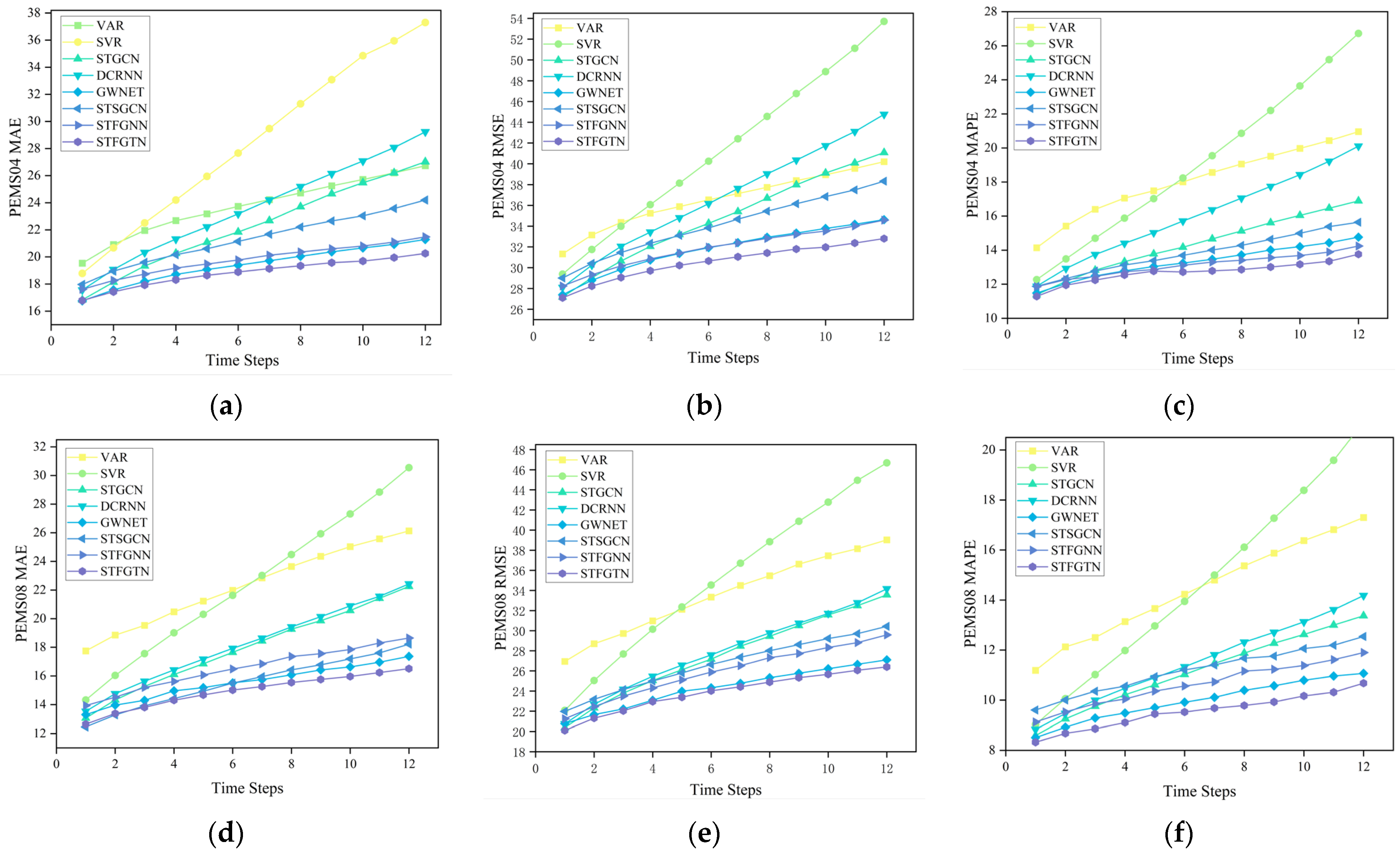
Figure 4 illustrates the performance comparison of our model with different types of methods over 12 time steps on the PEMS04 and PEMS08 datasets. Generally, as the prediction interval increases, the task becomes more challenging, resulting in performance degradation across all models. However, our model, STFGTN, exhibits the smallest decrease in performance compared to both GNN-based and attention-based models, highlighting its superiority in long-term prediction among other models. This also demonstrates the effectiveness of the improvements made on our proposed Transformer-based model.
5.5. Ablation Study
In order to further assess the validity of each component of STFGTN, we conducted an ablation study of four variants of our model on the PEMS04 and PEMS08 datasets:
- w/o s_gate: this variant removes the spatial fusion gating and simply splices the GCN with the output of spatial attention.
- w/o st_fusion_gate: this variant removes the spatial–temporal fusion gating mechanism and splices the output of fused spatial features with temporal attention.
- w/o Ttrans: this variant removes the time transformer.
- w/o Strans: this variant removes the spatial transformer.
Figure 5 illustrates a comparison of these variants, from which we draw the following conclusions: the integration of these components enables improved capture of spatial–temporal interaction information, validating the effectiveness of the overall model framework. The significant degradation in model performance upon removing the temporal and spatial attention mechanisms, respectively, indicates their crucial roles in capturing remote temporal dependencies across the temporal dimension and global spatial dependencies among different roads in the spatial dimension. In terms of spatial fusion, the effect of the spatial fusion gating mechanism is important for adjusting spatial information, and its absence leads to a decrease in model performance. By introducing the gating nonlinearity, the model can capture spatial and temporal dependence more flexibly, significantly improving the modeling effect.
By conducting a comparative analysis of replacing dynamic GCN with traditional GCN, as shown in Table 5, we are able to more clearly evaluate the role and effectiveness of dynamic GCN in our model. Traditional GCNs use static graphs to initialize relationships between nodes, while dynamic GCNs initialize them based on the road matrix during the initialization phase. Through attention mechanisms, the model’s weight matrices can dynamically adjust, focusing attention on the nodes and features most relevant to the prediction task. Additionally, by stacking multiple GCN layers, the model can gradually extract higher-level feature representations, thereby improving the model’s representation capability and prediction performance.
5.6. Visualization
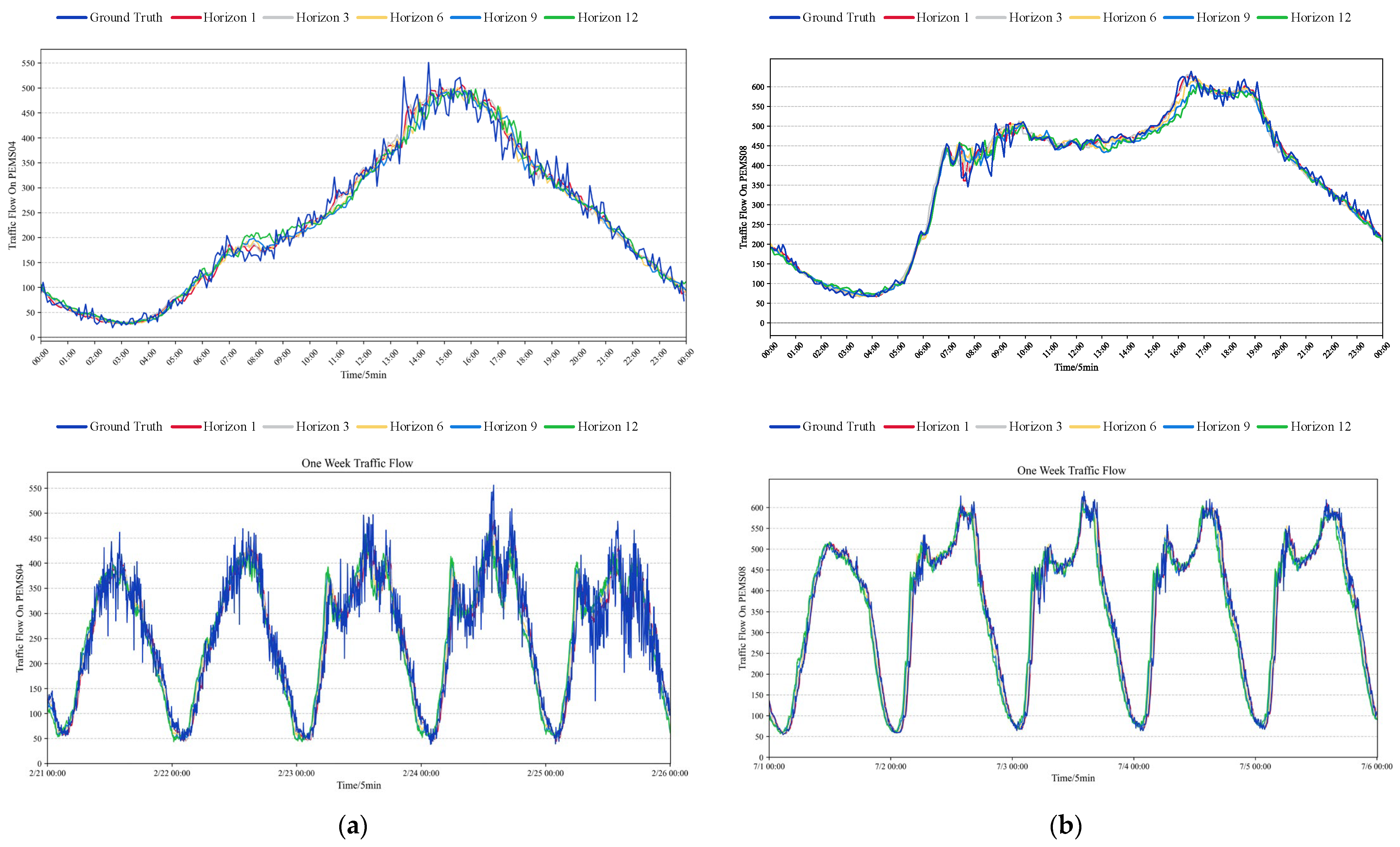
To demonstrate the prediction performance of our model, we conducted predictions on the test sets of sensor 100 from the PeMS04 dataset and sensor 80 from the PeMS08 dataset for both daily and weekly traffic flows. Figure 6 depicts that our predicted sequences closely align with the actual traffic flow on both the fitting curves for the PEMS04 and PEMS08 datasets, maintaining consistency despite variations in the field of view. This indicates that our model accurately forecasts by comprehensively considering the traffic flow characteristics within the real road network.
Figure 7 and Figure 8 display the absolute error of STFGTN for the 15 min, 30 min, 45 min, and 60 min prediction tasks on PEMS04 and PEMS08.
The model demonstrates proficiency in both short-term and long-term forecasting, effectively capturing temporal trends within traffic flow data. Nonetheless, its predictive efficacy diminishes with an extended prediction horizon, attributed to the heightened complexity and variability inherent in actual traffic conditions.
5.7. Effect of Hyperparameters
In our study, we explored the impact of variations in hyperparameters, including the number of attention heads, the number of layers in the spatiotemporal module, and changes in dimensionality.
In Figure 9, we observe a clear trend in traffic flow prediction performance as model dimensionality increases. Initially, there is a decrease followed by improvement. Notably, optimal performance is achieved at a dimensionality of 64, attributed to the model’s enhanced capability in capturing intricate traffic data features while mitigating overfitting risks. However, escalating model dimensionality may exacerbate overfitting and computational complexity, adversely affecting overall performance and generalization ability.
In Table 6 and Table 7, we looked at the effects of the number of attention heads and the number of layers of the spatial–temporal module on the performance of the STFGTN (h, l), where h is the number of heads of attention and l is the number of layers of the ST-block. The (*) indicates the parameter settings at which our model achieved optimal performance. The observed results show a gradual increase in model performance at the beginning of the increase in the number of attention heads. However, when the number of heads reaches eight, we observe a significant decrease in model performance. This phenomenon suggests that multi-head attention does not significantly improve the accuracy of traffic flow prediction. Conversely, an excessive number of attention heads introduces redundant information, potentially leading to overfitting or underutilization of the attention mechanism when dealing with traffic flow.
Similarly, for the number of layers of the spatial–temporal module, we find that the model achieves optimal performance at a layer number of three. However, as the number of layers increases to four, the model performance starts to show a decreasing trend. This suggests to us that increasing the number of layers in the spatial–temporal module does not lead to additional performance gains, but instead may introduce too much complexity and reduce computational efficiency, making the model too deep to train or generalize when dealing with spatial–temporal relationships.
6. Conclusions
In this study, we introduced a traffic flow prediction model that integrates spatial–temporal features using attention mechanisms. In this model, an embedding layer is utilized to incorporate periodic time features, and a spatial fusion gating module is proposed to integrate spatial dependencies and a spatial–temporal bilinear gating module to combine spatial–temporal dependencies. Further improvements were made to the original GCN by combining it with an attention mechanism to learn different spatial dependency patterns. The experiments were performed on four real datasets, experiments on ablation and parametric aspects of the individual modules were performed, and the results demonstrate the superiority of our model. In future work, we plan to explore the replacement of attention mechanisms and their broader application in the field of traffic flow prediction. We will particularly focus on investigating the impact of different types of attention mechanisms on model performance and generalization ability, aiming to further enhance the adaptability and prediction accuracy of the models in new environments.
Author Contributions
Writing—original draft preparation, H.X.; methodology, H.X.; software, H.X.; validation, H.X. and X.F.; formal analysis, H.X. and X.F.; data curation, X.F.; writing—review and editing, D.W. and K.Q.; supervision, C.R. All authors have read and agreed to the published version of the manuscript.
Funding
This research was funded by the Youth Innovation Team Development Plan of Shandong Province Higher Education (No. 2019KJN048).
Institutional Review Board Statement
Not applicable.
Data Availability Statement
The data presented in this study are available on request from the corresponding author.
Conflicts of Interest
Author Kaiyuan Qi and Dong Wu was employed by the company Inspur (Jinan) Data Technology Co., Ltd. The remaining authors declare that the research was conducted in the absence of any commercial or financial relationships that could be construed as a potential conflict of interest”.
References
- Yin, C.; Xiong, Z.; Chen, H.; Wang, J.; Cooper, D.; David, B. A literature survey on smart cities. Sci. China Inf. Sci. 2015, 58, 1–18. [Google Scholar] [CrossRef]
- Tedjopurnomo, D.A.; Bao, Z.; Zheng, B.; Choudhury, F.M.; Qin, A.K. A Survey on Modern Deep Neural Network for Traffic Prediction: Trends, Methods and Challenges. IEEE Trans. Knowl. Data Eng. 2022, 34, 1544–1561. [Google Scholar] [CrossRef]
- Wang, J.; Jiang, J.; Jiang, W.; Li, C.; Zhao, W.X. LibCity: An Open Library for Traffic Prediction. In Proceedings of the 29th International Conference on Advances in Geographic Information Systems, Beijing, China, 2–5 November 2021; pp. 145–148. [Google Scholar]
- Petrlik, J.; Fucik, O.; Sekanina, L. Multi objective selection of input sensors for SVR applied to road traffic prediction. In Proceedings of the International Conference on Parallel Problem Solving from Nature, Ljubljana, Slovenia, 13–17 September 2014; Springer: Cham, Switzerland, 2014; Volume 8672, pp. 79–90. [Google Scholar]
- Westgate, B.S.; Woodard, D.B.; Matteson, D.S.; Henderson, S.G. Travel time estimation for ambulances using Bayesian data augmentation. Ann. Appl. Stat. 2013, 7, 1139–1161. [Google Scholar] [CrossRef]
- Paliwal, C.; Bhatt, U.; Biyani, P.; Rajawat, K. Traffic estimation and prediction via online variational Bayesian subspace filtering. IEEE Trans. Intell. Transp. Syst. 2021, 1, 1–11. [Google Scholar] [CrossRef]
- Zivot, E.; Wang, J. Vector Autoregressive Models for Multivariate Time Series; Springer: New York, NY, USA, 2003; pp. 385–427. [Google Scholar]
- Zhang, J.; Zheng, Y.; Qi, D. Deep spatio-temporal residual networks for citywide crowd flows prediction. Proc. AAAI Conf. Artif. Intell. 2017, 31, 1655–1661. [Google Scholar] [CrossRef]
- Yao, H.; Tang, X.; Wei, H.; Zheng, G.; Li, Z. Deep STN+: Context-aware spatial-temporal neural network for crowd flow prediction in metropolis. Proc. AAAI Conf. Artif. Intell. 2019, 33, 1020–1027. [Google Scholar]
- Yao, H.; Wu, F.; Ke, J.; Tang, X.; Jia, Y.; Lu, S.; Gong, P.; Ye, J.; Li, Z. Deep multi-view spatial-temporal network for taxi demand prediction. Proc. AAAI Conf. Artif. Intell. 2019, 32, 2588–2595. [Google Scholar] [CrossRef]
- Shi, X.; Chen, Z.; Wang, H.; Yeung, D.-Y.; Wong, W.-K.; Woo, W.-C. Convolutional LSTM network: A machine learning approach for precipitation nowcasting. Proc. NeurIPS. 2015, 28, 802–810. [Google Scholar]
- Wang, Y.; Long, M.; Wang, J.; Gao, Z.; Yu, P.S. Predrnn: Recurrent neural networks for predictive learning using spatio-temporal lstms. Proc. NeurIPS. 2017, 30, 879–888. [Google Scholar]
- Geng, X.; Li, Y.; Wang, L.; Zhang, L.; Yang, Q.; Ye, J.; Liu, Y. Spatiotemporal multi-graph convolution network for ride-hailing demand forecasting. Proc. AAAI Conf. Artif. Intell. 2019, 33, 3656–3663. [Google Scholar] [CrossRef]
- Li, M.; Zhu, Z. Spatial-temporal fusion graph neural networks for traffic flow forecasting. Proc. AAAI Conf. Artif. Intell. 2021, 35, 4189–4196. [Google Scholar] [CrossRef]
- Wu, Z.; Pan, S.; Long, G.; Jiang, J.; Zhang, C. Graph WaveNet for Deep Spatial-Temporal Graph Modeling. In Proceedings of the International Joint Conference on Artificial Intelligence 2020, Virtual, 7–15 January 2021; pp. 1907–1913. [Google Scholar]
- Wu, Z.; Pan, S.; Long, G.; Jiang, J.; Chang, X.; Zhang, C. Connecting the dots: Multivariate time series forecasting with graph neural networks. In Proceedings of the KDD 2‘0: The 26th ACM SIGKDD Conference on Knowledge Discovery and Data Mining, Virtual, 6–10 July 2020; pp. 753–763. [Google Scholar]
- Guo, S.; Lin, Y.; Feng, N.; Song, C.; Wan, H. Attention based spatial-temporal graph convolutional networks for traffic flow forecasting. Proc. AAAI Conf. Artif. Intell. 2019, 33, 922–929. [Google Scholar] [CrossRef]
- Wen, T.; Chen, E.; Chen, Y. Tensor-view Topological Graph Neural Network. arXiv 2024, arXiv:2401.12007. [Google Scholar]
- Subramonian, A.; Kang, J.; Sun, Y. Theoretical and Empirical Insights into the Origins of Degree Bias in Graph Neural Networks. arXiv 2024, arXiv:2404.03139. [Google Scholar]
- Subram Zhao, J.; Zhou, Z.; Guan, Z.; Zhao, W.; Ning, W.; Qiu, G.; He, X. IntentGC: A scalable graph convolution framework fusing heterogeneous information for recommendation. In Proceedings of the KDD 1‘9: The 25th ACM SIGKDD Conference on Knowledge Discovery and Data Mining, Anchorage, AK, USA, 4–8 August 2019; pp. 2347–2357. [Google Scholar]
- Bai, L.; Yao, L.; Li, C.; Wang, X.; Wang, C. Adaptive Graph Convolutional Recurrent Network for Traffic Forecasting. Proc. NeurIPS Conf. 2020, 33, 17804–17815. [Google Scholar]
- Zhang, J.; Zheng, Y. Traffic Flow Forecasting with Spatial-Temporal Graph Diffusion Network. Proc. AAAI Conf. Artif. Intell. 2021, 35, 15008–15015. [Google Scholar] [CrossRef]
- Ye, J.; Sun, L.; Du, B.; Fu, Y.; Xiong, H. Coupled Layer-wise Graph Convolution for Transportation Demand Prediction. Proc. AAAI Conf. Artif. Intell. 2021, 35, 4617–4625. [Google Scholar] [CrossRef]
- Liu, D.; Wang, J.; Shang, S.; Han, P. MSDR: Multi-Step Dependency Relation Networks for Spatial Temporal Forecasting. In Proceedings of the KDD 2‘2: The 28th ACM SIGKDD Conference on Knowledge Discovery and Data Mining, Washington, DC, USA, 14–18 August 2022; pp. 1042–1050. [Google Scholar]
- Mao, X.; Wan, H. GMDNet: A graph-based mixture density network for estimating packages’ multimodal travel time distribution. Proc. AAAI Conf. Artif. Intell. 2023, 37, 4561–4568. [Google Scholar] [CrossRef]
- Zheng, C.; Fan, X.; Wang, C.; Qi, J. GMAN: A Graph Multi-Attention Network for Traffic Prediction. Proc. AAAI Conf. Artif. Intell. 2020, 34, 1234–1241. [Google Scholar] [CrossRef]
- Guo, S.; Lin, Y.; Wan, H.; Li, X.; Cong, G. Learning Dynamics and Heterogeneity of Spatial-Temporal Graph Data for Traffic Forecasting. IEEE Trans. Knowl. Data Eng. 2021, 34, 5415–5428. [Google Scholar] [CrossRef]
- Lan, S.; Ma, Y. DSTAGNN: Dynamic Spatial-Temporal Aware Graph Neural Network for Traffic Flow Forecasting. Proc. 39th Int. Conf. Mach. Learn. 2022, 162, 11906–11917. [Google Scholar]
- Jin, D.; Shi, J. Trafformer: Unify Time and Space in Traffic Prediction. Proc. AAAI Conf. Artif. Intell. 2023, 37, 8114–8122. [Google Scholar] [CrossRef]
- Bruna, J.; Zaremba, W.; Szlam, A.; LeCun, Y. Spectral networks and locally connected networks on graphs. arXiv 2013, arXiv:1312.6203. [Google Scholar]
- Defferrard, M.; Bresson, X.; Vandergheynst, P. Convolutional neural networks on graphs with fast localized spectral filtering. Proc. NeurIPS Conf. 2016, 29, 3844–3852. [Google Scholar]
- Kipf, T.N.; Welling, M. Semi-supervised classification with graph convolutional networks. arXiv 2016, arXiv:1609.02907. [Google Scholar]
- Veličković, P.; Cucurull, G.; Casanova, A.; Romero, A.; Lio, P.; Bengio, Y. Graph attention networks. arXiv 2017, arXiv:1710.10903. [Google Scholar]
- Xing, Z.; Huang, M.; Li, W. Spatial linear transformer and temporal convolution network for traffic flow prediction. Sci. Rep. 2024, 14, 4040. [Google Scholar] [CrossRef]
- Liu, Z.; Lin, Y.; Cao, Y.; Hu, H.; Wei, Y.; Zhang, Z.; Lin, S.; Guo, B. Swin transformer: Hierarchical vision transformer using shifted windows. In Proceedings of the IEEE/CVF International Conference on Computer Vision, Virtual, 11–17 October 2021; pp. 10012–10022. [Google Scholar]
- Jiang, J.; Han, C.; Zhao, W.X.; Wang, J. PDFormer: Propagation Delay-aware Dynamic Long-range Transformer for Traffic Flow Prediction. Proc. AAAI Conf. Artif. Intell. 2023, 37, 4365–4373. [Google Scholar] [CrossRef]
- Yan, H.; Ma, X. Learning dynamic and hierarchical traffic spatiotemporal features with Transformer. arXiv 2021, arXiv:2104.05163. [Google Scholar] [CrossRef]
- Cai, L.; Janowicz, K.; Mai, G.; Yan, B.; Zhu, R. Traffic transformer: Capturing the continuity and periodicity of time series for traffic forecasting. Trans. GIS 2020, 24, 736–755. [Google Scholar] [CrossRef]
- Vaswani, A.; Shazeer, N.; Parmar, N.; Uszkoreit, J.; Jones, L.; Gomez, A.N.; Kaiser, Ł.; Polosukhin, I. Attention is all you need. Adv. Neural Inf. Process. Syst. 2017, 30, 5998–6008. [Google Scholar]
- Yu, B.; Yin, H.; Zhu, Z. Spatio-temporal graph convolutional networks: A deep learning framework for traffic forecasting. arXiv 2017, arXiv:1709.04875. [Google Scholar]
- Song, C.; Lin, Y.; Guo, S.; Wan, H. Spatial-temporal synchronous graph convolutional networks: A new framework for spatial-temporal network data forecasting. Proc. AAAI Conf. Artif. Intell. 2020, 34, 914–921. [Google Scholar] [CrossRef]
- Li, Y.; Yu, R.; Shahabi, C.; Liu, Y. Diffusion Convolutional Recurrent Neural Network: Data-Driven Traffic Forecasting. In Proceedings of the 6th International Conference on Learning Representations, ICLR 2018, Vancouver, BC, Canada, 30 April–3 May 2018. [Google Scholar]
- Fang, Z.; Long, Q.; Song, G.; Xie, K. Spatial Temporal Graph ODE Networks for Traffic Flow Forecasting. In Proceedings of the KDD 2‘1: The 27th ACM SIGKDD Conference on Knowledge Discovery and Data Mining, Virtual, 14–18 August 2021; pp. 364–373. [Google Scholar]
- Choi, J.; Choi, H.; Hwang, J.; Park, N. Graph Neural Controlled Differential Equations for Traffic Forecasting. Proc. AAAI Conf. Artif. Intell. 2022, 36, 6367–6374. [Google Scholar] [CrossRef]
- Han, L.; Ma, X.; Sun, L.; Du, B.; Fu, Y.; Lv, W.; Xiong, H. Continuous-Time and Multi-Level Graph Representation Learning for Origin-Destination Demand Prediction. In Proceedings of the KDD 2‘2: The 28th ACM SIGKDD Conference on Knowledge Discovery and Data Mining, Washington, DC, USA, 14–18 August 2022; pp. 145–148. [Google Scholar]
- Yu, Q.; Ding, W.; Sun, M.; Huang, J. An Evolving Transformer Network Based on Hybrid Dilated Convolution for Traffic Flow Prediction. Collab. Com. 2024, 563, 329–343. [Google Scholar]
- Yun, I.; Shin, C.; Lee, H.; Lee, H.-J.; Rhee, C.E. EGformer: Equirectangular Geometry-biased Transformer for 360 Depth Estimation. In Proceedings of the IEEE/CVF International Conference on Computer Vision, Paris, France, 2–6 October 2023; pp. 6101–6112. [Google Scholar]
- Alshehri, A.; Owais, M.; Gyani, J.; Aljarbou, M.H.; Alsulamy, S. Residual Neural Networks for Origin–Destination Trip Matrix Estimation from Traffic Sensor Information. Sustainability 2024, 15, 9881. [Google Scholar] [CrossRef]
- Owais, M. Deep Learning for Integrated Origin–Destination Estimation and Traffic Sensor Location Problems. IEEE Trans. 2024, 1–13. [Google Scholar] [CrossRef]
Figure 1.
(a) This is a real-time road condition map from the high-speed highway traffic detection system in the Los Angeles area. The system installs detectors in various areas of the road to collect real-time traffic flow data. These data include metrics such as vehicle speed, vehicle density, traffic volume, etc., along with their variations over time and spatial locations. (b) Scenario of traffic flow correlations and heterogeneity in the road network. The traffic condition at one node will influence other nodes over time and space.

Figure 2.
Framework of the STFGTN. Comprising a data embedding layer, several stacked spatiotemporal modules, and an output layer.
Figure 2.
Framework of the STFGTN. Comprising a data embedding layer, several stacked spatiotemporal modules, and an output layer.

Figure 3.
The structure of the spatial–temporal block. (a) The spatial–temporal block. (b) The two gating modules used for fusing spatial–temporal features are respectively referred to as the Spatial Fusion Gate and Spatial–Temporal Fusion Gate.
Figure 3.
The structure of the spatial–temporal block. (a) The spatial–temporal block. (b) The two gating modules used for fusing spatial–temporal features are respectively referred to as the Spatial Fusion Gate and Spatial–Temporal Fusion Gate.

Figure 4.
The performance of different models on two datasets then varies at different time steps. (a–c) This represents the performance difference of STFGTN compared to other baseline models across different time steps in the PEMS04 dataset; (d–f) this represents the performance difference of STFGTN compared to other baseline models across different time steps in the PEMS08 dataset.

Figure 5.
Ablation study on PEMS04 and PEMS08. (a–c) This represents the performance variation of each key component across different evaluation metrics in the PEMS08 dataset; (d–f) this represents the performance variation of each key component across different evaluation metrics in the PEMS04 dataset.

Figure 6.
Visualization of traffic flow. (a) The fitting curve plot of sensor 100 in the PEMS04 dataset. (b) The fitting curve plot of sensor 80 in the PEMS08 dataset.
Figure 6.
Visualization of traffic flow. (a) The fitting curve plot of sensor 100 in the PEMS04 dataset. (b) The fitting curve plot of sensor 80 in the PEMS08 dataset.

Figure 7.
Heatmap shows the absolute errors between true and predicted values for different prediction horizons on PEMS04.
Figure 7.
Heatmap shows the absolute errors between true and predicted values for different prediction horizons on PEMS04.

Figure 8.
Heatmap shows the absolute errors between true and predicted values for different prediction horizons on PEMS08.
Figure 8.
Heatmap shows the absolute errors between true and predicted values for different prediction horizons on PEMS08.

Figure 9.
Different dimensions’ performance on different datasets: (a) Performance graph of different dimensions on PEMS04 dataset. (b) Performance graph of different dimensions on PEMS08 dataset.
Figure 9.
Different dimensions’ performance on different datasets: (a) Performance graph of different dimensions on PEMS04 dataset. (b) Performance graph of different dimensions on PEMS08 dataset.


Table 1.
Summary of datasets.
| Datasets | Nodes | Timesteps | Time Range |
|---|---|---|---|
| PEMS04 | 307 | 16,992 | 1/1/2018–2/28/2018 |
| PEMS07 | 883 | 28,224 | 5/1/2017–8/31/2017 |
| PEMS08 | 170 | 17,856 | 7/1/2016–8/31/2016 |
| PEMS-BAY | 325 | 52,116 | 1/1/2017–5/1/2017 |
Table 2.
Performance on PEMS04, PEMS07, and PEMS08.
| Model | PEMS04 | PEMS07 | PEMS08 | ||||||
|---|---|---|---|---|---|---|---|---|---|
| MAE | MAPE (%) | RMSE | MAE | MAPE (%) | RMSE | MAE | MAPE (%) | RMSE | |
| VAR | 23.750 | 18.090 | 36.660 | 101.200 | 39.690 | 155.140 | 22.320 | 14.470 | 33.830 |
| SVR | 28.660 | 19.150 | 44.590 | 32.970 | 15.430 | 50.150 | 23.250 | 14.710 | 36.150 |
| DCRNN | 22.737 | 14.751 | 36.575 | 23.634 | 12.281 | 36.514 | 18.185 | 11.235 | 28.176 |
| STGCN | 21.758 | 13.874 | 34.769 | 22.898 | 11.983 | 35.440 | 17.838 | 11.235 | 27.122 |
| GWNET | 19.358 | 13.301 | 31.719 | 21.221 | 9.075 | 34.117 | 15.063 | 11.211 | 24.855 |
| MTGNN | 19.076 | 12.964 | 31.564 | 20.824 | 9.032 | 34.087 | 15.396 | 9.514 | 24.934 |
| STSGCN | 21.185 | 13.882 | 33.649 | 24.264 | 10.204 | 39.034 | 17.133 | 10.170 | 36.785 |
| STFGNN | 19.830 | 13.021 | 31.870 | 22.072 | 9.212 | 35.805 | 16.636 | 10.961 | 26.206 |
| STGODE | 20.849 | 13.781 | 32.825 | 22.976 | 10.142 | 36.190 | 16.819 | 10.547 | 26.240 |
| STGNCDE | 19.211 | 12.772 | 31.088 | 20.620 | 8.864 | 34.036 | 15.455 | 10.623 | 24.813 |
| GMAN | 19.139 | 13.192 | 31.601 | 20.967 | 9.052 | 34.097 | 16.819 | 10.134 | 24.915 |
| TFormer | 18.916 | 12.711 | 31.349 | 20.754 | 8.972 | 34.062 | 15.455 | 9.925 | 24.883 |
| STFGTN | 18.829 | 12.703 | 30.532 | 20.549 | 8.673 | 33.802 | 14.987 | 9.638 | 23.950 |
Table 3.
Performance on PEMS-BAY.
| Datasets | Metric | DCRNN | STGCN | MTGNN | GMAN | STFGTN | |
|---|---|---|---|---|---|---|---|
| PEMS-BAY | Horizon 3 (15 min) | MAE | 1.38 | 1.36 | 1.33 | 1.35 | 1.33 |
| RMSE | 2.95 | 2.96 | 2.80 | 2.90 | 2.85 | ||
| MAPE | 2.90% | 2.90% | 2.81% | 2.87% | 2.83% | ||
| Horizon 6 (30 min) | MAE | 1.74 | 1.81 | 1.66 | 1.65 | 1.63 | |
| RMSE | 3.97 | 4.27 | 3.77 | 3.82 | 3.70 | ||
| MAPE | 3.90% | 4.17% | 3.75% | 3.74% | 3.63% | ||
| Horizon 9 (60 min) | MAE | 2.07 | 2.49 | 1.95 | 1.92 | 1.90 | |
| RMSE | 4.74 | 5.69 | 4.50 | 4.49 | 4.38 | ||
| MAPE | 4.90% | 5.79% | 4.62% | 4.52% | 4.44% |
Table 4.
Performance of the transformer-based model on the PEMS04 and PEMS08 datasets.
| Model | PEMS04 | PEMS08 | ||||
|---|---|---|---|---|---|---|
| MAE | MAPE (%) | RMSE | MAE | MAPE (%) | RMSE | |
| GMAN | 19.139 | 13.192 | 31.601 | 16.819 | 10.134 | 24.915 |
| TFormer | 18.916 | 12.711 | 31.349 | 15.455 | 9.925 | 24.883 |
| DSTAGNN | 19.304 | 12.700 | 31.460 | 15.671 | 9.943 | 24.772 |
| HDCFormer | 32.806 | 16.154 | 43.602 | 15.715 | 10.612 | 20.543 |
| EGFormer | 29.796 | 14.792 | 40.822 | 31.523 | 11.386 | 44.104 |
| STFGTN | 18.829 | 12.703 | 30.532 | 14.987 | 9.638 | 23.950 |
Table 5.
Performance of traditional GCN and DGCN on the PEMS04 and PEMS08 datasets.
| Datasets | Metrics | Classical GCN | DGCN |
|---|---|---|---|
| PEMS04 | MAE | 19.263 | 18.829 |
| MAPE(%) | 13.038 | 12.703 | |
| RMSE | 31.074 | 30.532 | |
| PEMS08 | MAE | 15.597 | 14.987 |
| MAPE(%) | 10.058 | 9.638 | |
| RMSE | 24.614 | 23.950 |
Table 6.
Examines the fluctuations in MAE, MAPE (%), and RMSE acquired by STFGTN (h, l) with varying numbers of attention heads and layers of ST-block in the PEMS04 dataset.
Table 6.
Examines the fluctuations in MAE, MAPE (%), and RMSE acquired by STFGTN (h, l) with varying numbers of attention heads and layers of ST-block in the PEMS04 dataset.
| PEMS04 | |||
|---|---|---|---|
| Model | MAE | MAPE (%) | RMSE |
| STFGTN (2, 3) * | 18.829 | 12.703 | 30.532 |
| STFGTN (1, 3) | 19.111 | 12.886 | 31.561 |
| STFGTN (4, 3) | 18.962 | 12.679 | 31.086 |
| STFGTN (8, 3) | 18.962 | 12.795 | 31.122 |
| STFGTN (2, 1) | 20.076 | 13.571 | 32.520 |
| STFGTN (2, 2) | 19.164 | 13.329 | 31.024 |
| STFGTN (2, 4) | 19.195 | 12.760 | 31.362 |
Table 7.
Examines the fluctuations in MAE, MAPE (%), and RMSE acquired by STFGTN (h, l) with varying numbers of attention heads and layers of ST-block in the PEMS08 dataset.
Table 7.
Examines the fluctuations in MAE, MAPE (%), and RMSE acquired by STFGTN (h, l) with varying numbers of attention heads and layers of ST-block in the PEMS08 dataset.
| PEMS08 | |||
|---|---|---|---|
| Model | MAE | MAPE (%) | RMSE |
| STFGTN (2, 3) * | 14.987 | 9.638 | 23.950 |
| STFGTN (1, 3) | 15.511 | 10.014 | 24.619 |
| STFGTN (4, 3) | 15.097 | 9.965 | 23.992 |
| STFGTN (8, 3) | 15.203 | 10.045 | 24.152 |
| STFGTN (2, 1) | 16.033 | 10.260 | 24.330 |
| STFGTN (2, 2) | 15.337 | 9.981 | 31.024 |
| STFGTN (2, 4) | 15.097 | 9.651 | 23.992 |
Disclaimer/Publisher’s Note: The statements, opinions and data contained in all publications are solely those of the individual author(s) and contributor(s) and not of MDPI and/or the editor(s). MDPI and/or the editor(s) disclaim responsibility for any injury to people or property resulting from any ideas, methods, instructions or products referred to in the content. |
© 2024 by the authors. Licensee MDPI, Basel, Switzerland. This article is an open access article distributed under the terms and conditions of the Creative Commons Attribution (CC BY) license (https://creativecommons.org/licenses/by/4.0/).
Share and Cite
MDPI and ACS Style
Xie, H.; Fan, X.; Qi, K.; Wu, D.; Ren, C. Spatial–Temporal Fusion Gated Transformer Network (STFGTN) for Traffic Flow Prediction. Electronics 2024, 13, 1594. https://doi.org/10.3390/electronics13081594
AMA Style
Xie H, Fan X, Qi K, Wu D, Ren C. Spatial–Temporal Fusion Gated Transformer Network (STFGTN) for Traffic Flow Prediction. Electronics. 2024; 13(8):1594. https://doi.org/10.3390/electronics13081594
Chicago/Turabian StyleXie, Haonan, Xuanxuan Fan, Kaiyuan Qi, Dong Wu, and Chongguang Ren. 2024. "Spatial–Temporal Fusion Gated Transformer Network (STFGTN) for Traffic Flow Prediction" Electronics 13, no. 8: 1594. https://doi.org/10.3390/electronics13081594
Note that from the first issue of 2016, this journal uses article numbers instead of page numbers. See further details here.