Article

Modeling of Induction Motors and Variable Speed Drives for Multi-Domain System Simulations Using Modelica and the OpenIPSL Library

by
Fernando Fachini
1,
Marcelo de Castro
2,
Tetiana Bogodorova
1 and
Luigi Vanfretti
1,*
1
Electrical, Computer and Systems Engineering Department, Rensselaer Polytechnic Institute, Troy, NY 12180, USA
2
Power Systems Engineering Department, Mitsubishi Electric Power Products, Inc., Warrendale, PA 15086, USA
*
Author to whom correspondence should be addressed.
Electronics 2024, 13(9), 1614; https://doi.org/10.3390/electronics13091614
Submission received: 19 March 2024 / Revised: 15 April 2024 / Accepted: 17 April 2024 / Published: 23 April 2024

Abstract

:
This paper introduces an innovative method for characterizing, implementing, and validating both three-phase and single-phase induction motor models, accompanied by a variable speed drive model. The primary goal is to investigate interactions between the electrical power grid and other dynamic domains (e.g., thermofluidic) that impact motor/load drive behavior. Our approach involves establishing a mechanical interface based on a physically meaningful equation linking motor torque/speed to the electrical model in the phasor domain. This allows seamless integration of diverse domain subsystems into a unified multi-domain model using Modelica v4.0.0 and the OpenIPSL library v3.0.1, overcoming co-simulation limitations. The proposed model, which requires only one Modelica-compliant tool for simulation, introduces additional dynamics through the mechanical interface, enabling explicit simulation of load disturbances based on constitutive physics. This deepens our understanding of dynamic interactions between the electrical power domain and other subsystems connected through the motor. We detail the modeled components using mathematical equations and textual descriptions, emphasizing the Modelica modeling approach. Simulation examples validate the implementation, demonstrating the multi-domain modeling capabilities of the newly developed components.

1. Introduction

1.1. Motivation

Electrical motors play a crucial role in converting electrical power into mechanical power for a wide range of applications, from handheld drills that use DC motors to massive industrial loads that use AC motors controlled by variable speed drives (VSDs). Their sizes vary significantly, with power consumption ranging from a few watts to thousands of kilowatts. According to the US Energy Information Administration (EIA), electrical motors collectively represented the largest share of electricity consumption by US manufacturers in 2018, representing approximately 51.6% of the total use of electricity in the industrial sector. Despite the long-standing knowledge and experience in the electrical machine sector, companies such as General Electric (GE) continue to improve motor efficiency and robustness. Notably, GE has recently introduced the world’s largest three-phase electrical motor, specifically designed for the liquefied natural gas (LNG) industry [1]. Given the importance of the induction motor in power system design and operation studies [2], power system simulation tools, such as Siemens PTI PSS® E [3], Power System Toolbox (PST) [4], Power System Analysis Toolbox (PSAT) [5], PowerWorld [6], and GE PSLF [7], all provide motor models that can simulate the dynamics of a three-phase induction motor in positive sequence phasor domain representation. The caveat to these induction motor models is that the driven load dynamics are simplified and represented by polynomial functions that are meant to “emulate” the load torque. This means that traditional induction motor modeling is detached from the physical representation of the load itself, and this is due to the modeling philosophy on which conventional power system tools were built. In fact, all physical domains that diverge from the electrical phasor domain representation of the motor are simplified by transfer functions that capture the dynamics of the main time constants of the real processes, efficiency expressions that substitute differential equation modeling, or even fitted polynomials [8]. While this approach is useful for macroscopic studies focused solely on the behavior of the power grid, it is insufficient for understanding more complex interactions driven by the actual dynamics of the loads. An example would be the creation of more substantial efficiencies and services from building-to-grid interactions by leveraging more microscopic control of the load behavior and that of the end user [9].
Over the years, the Western Electric Coordinating Council (WECC) has updated and proposed new load models for dynamic simulation of the power system, including a composite load model that aggregates motors and static loads into one single load model [10,11]. The composite load model can be used to represent residential, commercial, and industrial loads for dynamic studies by adjusting the built-in parameters of the model. Although it is an improvement over previous generations of load models, commercial power system tools are still limited when dealing with multiple domains, e.g., representing the underlying process driving the load using simplified mathematical expressions and not the process’ constitutive physics. In fact, a relevant example of the need to build more detailed motor models becomes clear when studying microgrids where the interaction of power and thermofluid systems exist [12]. Gas turbines, which are typically used in combined heat and power (CHP) plants, generate electricity, but also produce thermal energy, which is used to heat buildings within the microgrid. Electrical water pumps are utilized to transport heated fluid into buildings and also to pump it back to the thermal source (CHP). Thus, to model and study these multi-domain systems and processes, a motor model with its mechanical interface to connect with other domains is necessary. Therefore, in the process of developing motor models that display the mechanical interface, the term multi-domain model refers to the addition of a physically meaningful mechanical interface to the motor that allows it to be coupled to different domains represented by their constitutive physics. With the new addition to the motor model, the user can study the complex inter-domain interactions, creating a more comprehensive environment than traditional power system tools allow.
Instead of using common co-simulation approaches for the coupling of subsystems using different established tools for each specific domain [13], our aim is to integrate the subsystems into one monolithic model simulated in one tool using the Modelica language. In this way, one can avoid several limitations such as the following: (a) numerical stability issues of co-simulation, (b) difficulties in choosing the right co-simulation orchestration algorithm (master), and (c) difficulties in how to define the macro step size for a specific co-simulation, just to name a few [13]. Although the benefit of avoiding co-simulation is attractive, this implies that models not available in the Modelica language or provided as functional mock-up units for model exchange would need to be re-implemented in one of these standards, which naturally implies an investment of time and effort. While the simulation performance of Modelica-compliant tools has been a concern in the past [14], recent developments addressing this issue for large-scale complex models have resulted in major improvements [15], and the case of power systems, these tools are now as competitive as legacy domain-specific tools [16].
This work also implements a variable speed drive (VSD) model, which is not present in traditional power system analysis tools. Although VSDs are typically examined independently of the power grid by experts in power electronics, it is essential to recognize their significance in industrial settings as a means of regulating motor operations. This underscores the need for a suitable model, particularly when aiming to improve efficiency and services through interactions between buildings and the grid [9]. VSDs enhance motor performance by minimizing the potential for motor damage when starting and stopping, thus extending motor life, consequently decreasing the need for motor maintenance services, and improving energy conservation [17,18].
With this in mind, this article is focused on describing the implementation of the novel multi-domain models and the VSD drive, which were developed using the Modelica modeling language [19] and are compatible with the Open-Instance Power System Library (OpenIPSL) [20]. The Modelica language is an object-oriented multi-domain modeling language used to simulate complex cyber-physical systems [21], which allows for model representation in the form of equations, and seamless creation and connection of components from multiple different domains. OpenIPSL is an open-source Modelica-based library that was developed as an alternative to the standard commercial power system tools in the market.

1.2. Contributions

The current paper proposes the following contributions:
  • The implementation of phasor-based three-phase and single-phase multi-domain electrical motor models.
  • The implementation of a VSD model that allows for simulating the speed control operation over induction motors.
  • The description of a multi-domain model that illustrates the interaction between a thermofluidic system and the electrical grid.
These contributions will be expounded upon in the body of this manuscript, while a summary of each is described next.
In Contribution 1, the proposed models were developed so that they could be used in conventional power system simulations or multi-domain simulations. In the latter, the proposed models are capable of coupling the electrical domain (the motor and a three-phase VSD model for motor control studies) with the mechanical domain (the driven load). While the positive sequence modeling of motors is the de-facto modeling approach in dynamic power system tools, the motor model with an interface to couple with another domain using the Modelica language is novel and allows studying the dynamic interaction between the electrical and other domains.
In Contribution 2, we provide a capability that is neither found nor modeled in standard phasor domain dynamic power system tools. Because the new motor models can be coupled to the VSD model, this also implies that the motor models have frequency-varying stator and rotor impedances, which is also an improvement to the de-facto modeling approaches used by power system tools. Considering the numerous advantages of using the VSD in current induction motor applications, the proposed Modelica-based VSD model is a crucial addition for researchers studying interactions between the power grid and other energy systems.
Finally, in Contribution 3, the proposed two examples illustrate how the developed models allow for multi-domain modeling by including a thermofluidic system that is driven by a pump. In addition, it also displays the ability to couple components from different Modelica libraries into a single model thanks to the motor models developed in this paper.

1.3. Paper Organization

The remainder of this paper is divided into the following sections. Section 3 describes the Modelica modeling rationale used to develop the three- and single-phase induction motor models. Section 4 describes the implementation of the variable speed drive. Section 5 describes the validation process utilized for the motor models with multi-domain interfaces, simulations that test the performance of the motors, and multi-domain application examples. Finally, Section 6 presents the conclusions of this work and outlines future work.

2. Materials and Methods

It is strongly recommended that the reader refers to the actual implementation together with the presentation in this paper. The reader can access and test the models by downloading them from the following GitHub repository: OpenIMDML https://github.com/ALSETLab/OpenIMDML (accessed on 16 April 2024), and following the usage instructions described in [22].
Although the simulation results presented here were generated using the Dymola 2023x software [23], the repository tutorial provides instructions on how to run examples using OpenModelica, which is an open-source Modelica-compliant simulation environment [24].

3. Induction Motor Modeling

The industrial sector is the main electricity consumer in the world, consuming roughly half of the total power produced in the world. In countries such as the United States and Canada, of all industrial loads, electrical motors contribute approximately 75% of the consumed power [25]. Electrical motors convert electricity into driving torque, and most electrical motors can be grouped into two categories, namely alternate current (AC) and direct current (DC) motors. As their names imply, AC motors convert alternating voltage and current into mechanical power, while DC motors generate mechanical power out of direct voltage and current. From these two main categories, the AC induction motor is by far the most common and widely used type of electrical motor in residential, commercial, and industrial applications [25]. The induction motor requires a continuously rotating magnetic field in its stator to induce alternating current in the rotor circuit, which consequently induces electromagnetic torque. Of all the possible electrical motors, the induction motor is by far the most widely used type of electrical motor in industrial applications and is the main focus of the motor models developed. With the focal point of developing induction motor models in a multi-domain modeling environment that allows the coupling of multiple physical domains at once [26], the motor models described in this paper were developed to fill this gap.
The motor models described in this paper can be divided into two main categories, “non-multi-domain” (NMD) and “multi-domain”. The term “non-multi-domain” refers to models that represent mechanical loads according to power system modeling practices. Meanwhile, the term “multi-domain” (MD) refers to models with a physically meaningful equation-based interface that couples the motor shaft to a subsystem driven by the motor. Such a subsystem can be represented by a detailed dynamic model of the load, if desired.
  • Non-multi-domain (NMD) induction motor models: The non-multi-domain (NMD) group of models contains both single-phase and three-phase induction motor models. The single-phase induction motor models (single-phase induction motor model and the double-phase induction motor model) were derived from the “classic” Electric Machinery book by Fitzgerald [27], while the three-phase induction motor models (Type I, Type III, Type V, CIM5, and CIM6) were derived from the PSS® E and PSAT model manuals [3,8,28]. These NMD models do not include an interface for multi-domain (MD) modeling and, hence, are limited to the load torque polynomial function that is consistent with power system modeling practices. Nevertheless, to expand the features of these models, the implementation reported in this work is such that the impedances of the motor model vary with changing frequencies, i.e., they are frequency-dependent and not constant. Moreover, these models were used as a stepping stone toward the goal of implementing MD models, and since NMD and MD motor models have the electrical part in common with the difference in the mechanical interface, this paper focuses on describing the modeling process adopted to develop the MD models. Although the primary emphasis of this article lies in the development and elucidation of MD motor models, for completeness, Section 5.2 presents the validation results for the NMD CIM5 motor model.
  • Multi-domain (MD) induction motor models: The multi-domain (MD) group of models contains three-phase, single-phase, and double-phase MD induction motor models. These motor models were developed based on the description of the model in [3,8,28]; they were modified to account for changes in the impedance of the winding based on the change of the terminal voltage frequency and the mechanical interface that allows coupling with mechanical rotation components of the Modelica Standard Library (MSL) [29]. More details are provided in the following sections.
The electrical circuits of the induction motors described above are found in Appendix E. The following subsections detail the models, including the modeling structure of the motors developed. In order to avoid repetitiveness, the authors will exemplify the structure of the Modelica-based motor models through the description of one three-phase motor model, one single-phase, and a dual-phase motor.

3.1. Three-Phase Induction Motor Model

One of the key features of the Modelica modeling language is its object-oriented nature, which allows the extension of the behavior and properties of an existing class [19,21]. In Modelica (see the Modelica language specification: https://specification.modelica.org/ accessed on 16 April 2024). Each component of a model is presented as a class, and by using inheritance, a partial (the typewriter font is used to denote Modelica code and Modelica component names) class provides a base class from which a new class/model can be extended. The proposed three-phase induction motor models, whether multi-domain or not, have their own base class model. The following subsections are meant to explain the logic behind the base class and the extended model structure and elucidate the common characteristics between different induction motor models.

3.1.1. Base Class for Multi-Domain and Non-Multi-Domain Models

The NMD three-phase induction motor base class, named BaseNonMultiDomainThreePhase (the italic font is used to denote the names of the models that are being discussed), defines a common structure for all three-phase motor models, i.e., the basic equations that are ubiquitous to all three-phase NMD motor models. Similarly, the BaseMultiDomainThreePhase base model defines the common structure that is present in the developed MD three-phase motor models. Figure 1 depicts both the NMD and MD base classes in their “Icon” view (models in Modelica have multiple views or layers. The “Icon” view provides a user-facing graphical representation, the “Diagram” view is meant to graphically compose system models using multiple components, the “Text” view is where a component’s equations are defined, and the “Documentation” view provides information about the model. See the Modelica language specification: https://specification.modelica.org/ accessed on 16 April 2024).
Both base classes provide visual cues that help understand their modeling purposes; in particular, the red NMD acronym in the top left corner of the model stands for non-multi-domain, and the green MD acronym stands for multi-domain. More importantly, the NMD motor in Figure 1a has one physical (acasual) connector (pwpin) and two casual connectors (we, wr), where we is a RealInput connector that specifies the desired electrical speed and wr is a RealOuput connector that provides the mechanical rotor speed. Meanwhile, the MD motor in Figure 1b has the same acasual and casual connectors, in addition to an acasual connector (flange) and a casual connector (mech_torque), which are further explained below. The connector pwpin is an acasual connector specific to OpenIPSL, which is ubiquitous to all of the electrical component models in the library. It follows the grammar of several MSL subdomain packages, where the connector has potential and flow variables. In the case of OpenIPSL, the real and imaginary parts of the current that flow through the components arise from the real and imaginary parts of the voltage phasor values in the nodes of the system, defined by the buses [30].
While Figure 1 shows the icon view of the base class model, in Figure 2, the diagram view shows the structure of the base class model for the multi-domain version of the three-phase induction motor models.
The “Icon” view is the graphical representation of a model, and when dragged into a sub-system or system model, the user will interact with it (e.g., providing parameters). Meanwhile, the “Diagram” view shows how the model is composed of several other sub-components that are being used in the creation of the motor base class. For instance, in order for the model to interface with rotational components from the Modelica Standard Library, the rotor speed nr (which is calculated in the equation section of the base model within the “Text” view of the base component) is used as a reference value to the speed component, which forces the flange to rotate at the specified speed, converting the rotor speed nr into its equivalent torque and angle. For more information on the rotational components from the MSL and their modeling attributes, refer to [29].
Traditional power system stability software does not model motors as frequency and voltage-controlled equipment. However, in this work, both the NMD and MD models described in the work represent motor reactances based on the terminal bus frequency. The input connector we allows for adjusting the synchronous speed of the NMD motor model in rad/s, while the output connector wr is the resulting rotor speed in rad/s. In the case of traditional phasor domain power system tools, the impedance of all the components is tied to the system frequency (including the impedances in the motor), thus limiting motor simulations to grid-tied only. In contrast, the proposed motor models are more versatile, allowing for dynamic grid-tied motor simulation, grid-tied starting motor simulation, soft start motor simulation, and VSD-controlled motor simulation. All reactances of the rotor, stator, and magnetization windings vary with the frequency of the input voltage signal through the ratio w e X w b , where X represents reactances of the motor model and w b is the nominal synchronous speed of the electrical grid. For instance, the set of frequency-varying reactances of Motor Type III is defined as follows:
X m c o n t = w e w b X m n o m X s c o n t = w e w b X s n o m X r c o n t = w e w b X r n o m
where X m c o n t , X s c o n t , and X r c o n t are the frequency-varying magnetization, stator, and rotor reactances; X m n o m , X s n o m , and X r n o m are the nominal frequency magnetization, stator, and rotor reactance.
Exclusive to the MD model, its base class contains a flange connector port and the mech_torque input port. The acasual flange connector has a potential variable, which is the absolute rotation angle, and a flow variable, which is the cut torque. It is because of the flange connector that the model can be interfaced with rotational mechanical components from the MSL library [29], allowing the motor model to be coupled to any components with a matching flange connector. The load torque in the MD model is specified through mech_torque, which originates from a torque sensor that measures the torque in the MD load. The set of equations that define the base class model is shown in Listing 1.
Listing 1. Set of equations for the non-multi-domain and multi-domain motor base class in Modelica.
 (1) - Synchronous speed based on controllable boolean parameter
w_sync = (if Ctrl == true then we else w_b);
 (2) - Network Interface Equations
[Vr; Vi] = [p.vr; p.vi];
[Ir; Ii] = (1/CoB)*[p.ir; p.ii];
Imag = sqrt(Ir^2+Ii^2);
v = sqrt(p.vr^2+p.vi^2);
anglev = atan2(p.vi, p.vr);
 
 (3) - Active & Reactive Power Consumption on system base
P = p.vr*p.ir+p.vi*p.ii;
Q = (-p.vr*p.ii)+p.vi*p.ir;
 
 (4) - Active & Reactive Power Consumption on machine base
P_motor = P/CoB;
Q_motor = Q/CoB;
 
 (5) - Rotor speed equation
ns = w_sync/N;
nr = (1-s)*ns;
(6) - Conversion from SI torque to p.u. torque
Tmech_pu_sys = mech_torque/T_b;
Tmech_pu_motor = Tmech_pu_sys/CoB;
 (7) - Torque System base
T_b = S_b/w_b;
Listing 1 is the set of common equations from the BaseNonMultiDomainThreePhase and BaseMultiDomainThreePhase base models, and are divided into seven different sections.
  • Equation (1): Presents one equation that corresponds to the synchronous speed equation that enables all three-phase induction motor models from the library to be controllable. Ctrl is a user-defined Boolean parameter that, if chosen to be true, enables the motor model to connect to a motor control component, such as the VSD, and if deemed false, disables the controllable aspect of the motor model.
  • Equation (2): Defines the algebraic equations that are necessary for interfacing the motor model with power grid components through the pwpin connector that is instantiated as p with variables p.vr, p.vi, p.ir, and p.ii corresponding to the real and imaginary parts of the voltage and current at p.
  • Equation (3): Describes two algebraic equations that correspond to the active (P) and reactive power (Q) consumption of the motor model for the system’s apparent power base, linking the voltage and current variables from the pwpin connector.
  • Equation (4): Describes two algebraic equations for motor active and reactive power consumption, based on the motor’s apparent power base. Here, CoB is the motor change of the base from the system power base to the motor power base.
  • Equation (5): Defines the magnetic field synchronous speed ns and the effective rotor speed nr, respectively. The parameter N is the number of pairs of poles of the motor and s is the motor slip variable.
  • Equation (6): Specifies the mechanical torque expressed in per unit [ p . u . ] for the system base and the motor base. The variable T_b is the torque system base; it is used to convert mechanical torque from the Newton meter [ N . m ] to [ p . u . ].
  • Equation (7): Defines a system base torque value for unit conversion.
The next subsection explains how the base model is extended to create the three-phase induction MD and NMD motor models.

3.1.2. Creating Multi-Domain and Non-Multi-Domain Motor Models with Inheritance

This subsection describes the implementation of the extended MD model of the three-phase motor that applies to all its variants (see Appendix E, Figure A1a–d). In order to avoid repetitiveness, this subsection will only describe the model extension of the motor model Type III MD model. The modeling procedures for the other developed three-phase induction motor models are similar to the one described in this section and, thus, for the sake of brevity, they will be omitted.
As mentioned in the previous subsection, given the object-oriented nature of the Modelica modeling language, the creation of base classes allows us to define all common variables, parameters, equations, etc., which can be inherited in a new model class. As a result, the NMD AND ND motor models share the same icons in Figure 1 and equations as in Listing 1. Meanwhile, Listing 2 contains the set of complementary equations that uniquely defines the Type III induction motor model, divided into five sections.
Listing 2. Modelica set of equations for the three-phase multi-domain induction motor model type III.
 (8) - Rotor impedance based on controllable model
X0 = if Ctrl == false then Xs+Xm else (we_fix.y/w_b)*(Xs+Xm);
Xp = if Ctrl == false then Xs+X1*Xm/(X1+Xm) else we_fix.y*(Xs+X1*Xm/(X1+Xm))/w_b;
Tp0 = if Ctrl == false then (X1+Xm)/(w_b*R1) else (we_fix.y/w_b)*(X1+Xm)/(w_b*R1);
 
 (9) - The real and imaginary current relationship
Vr = epr+Rs*Ir-Xp*Ii;
Vi = epm+Rs*Ii+Xp*Ir;
 
 (10) - Electromagnetic differential equations
der(epr) = w_sync*s*epm-(epr+(X0-Xp)*Ii)/Tp0;
der(epm) = (-w_sync*s*epr)-(epm-(X0-Xp)*Ir)/Tp0;
 
 (11) - Mechanical Slip Equation
der(s) = (Tmech_pu_motor-Te_motor)/(2*H);
 
 (12) - Electromagnetic torque equation in system and machine base
Te_sys = Te_motor*CoB;
Te_motor = if Ctrl == false then (epr*Ir+epm*Ii) else (epr*Ir+epm*Ii)/(we_fix.y/w_b);
  • Equation (8): Defines two distinct induction motor reactance calculations, X0 and Xp, as well as an open-circuit time constant, Tp0, which are used to determine the real and imaginary components of the consumed current in Equation Set (9) and the change in real and imaginary voltages behind the stator resistance in Equation (10).
  • Equation (9): Defines two equations and two unknowns, namely Ir and Ii. The unknown variables are the real and imaginary parts of the consumed motor current, defining the current flow parameters from the pwpin connector. It is important to note that Vr and Vi (real and imaginary components of the motor terminal voltage) are potential parameters and are thus known at the initialization step of the simulation. The same can be said for the direct transient magnetization voltage epr and quadrature transient magnetization voltage epm.
  • Equation (10): Describes two differential equations for the direct transient magnetization voltage epr and quadrature transient magnetization voltage epm.
  • Equation (11): Describes the slip’s differential equation, representing the rate of change in the rotor speed as the motor drives a mechanical load. The slip is defined as the ratio between the mechanical and electromagnetic torque difference divided by double the motor’s inertia constant.
  • Equation (12): Defines the electromagnetic torque equation in both the system and machine bases.

3.2. All-in-One Multi-Domain and Non-Multi-Domain Motor Model

In order to encompass all types of three-phase induction motor model types (in Appendix E, see Figure A1a–d for a circuit diagram of the included models) into a single component, two models were developed, namely MultiDomainMotor and NonMultiDomainMotor. Both encompass one replaceable base class component, either NMD or MD. In Modelica, the replaceable keyword is used to designate components in a model whose type can be changed or redeclared, making the model reconfigurable [31].
The use of replaceable and redeclared allowed us to fully exploit the features of the object-oriented modeling language in Modelica to make the use of all variants of the model more accessible to the user. The user can, through one component only, choose which three-phase motor model type to utilize in the system’s simulation model, and whether or not to enable the multi-domain features. This makes it easier to use all available models from a user’s perspective, in addition to allowing the user to quickly modify the fidelity of the motor model without the need to change the system model.
The icon view of the MultiDomainMotor and NonMultiDomainMotor components are similar to the motor icon in Figure 1, differentiating itself with a written “ALL-IN-ONE” text in the icon. Figure 3 shows the parameter selection screen of the MultiDomainMotor motor model. The model contains four parameter groups:
  • Power flow data: Parameter section that defines the initialization values for the dynamic simulation. It is worth mentioning that it does not make sense to enable the user to input values to all parameters because the model is MD. Being MD, the initialization of the model is based on the mechanical model and not on solving a power flow [32]. Therefore, only the parameter M_b is enabled, allowing the user to change the value of the motor base power, while the rest are disabled and have a gray fill, indicating that they do not need to be provided to the user.
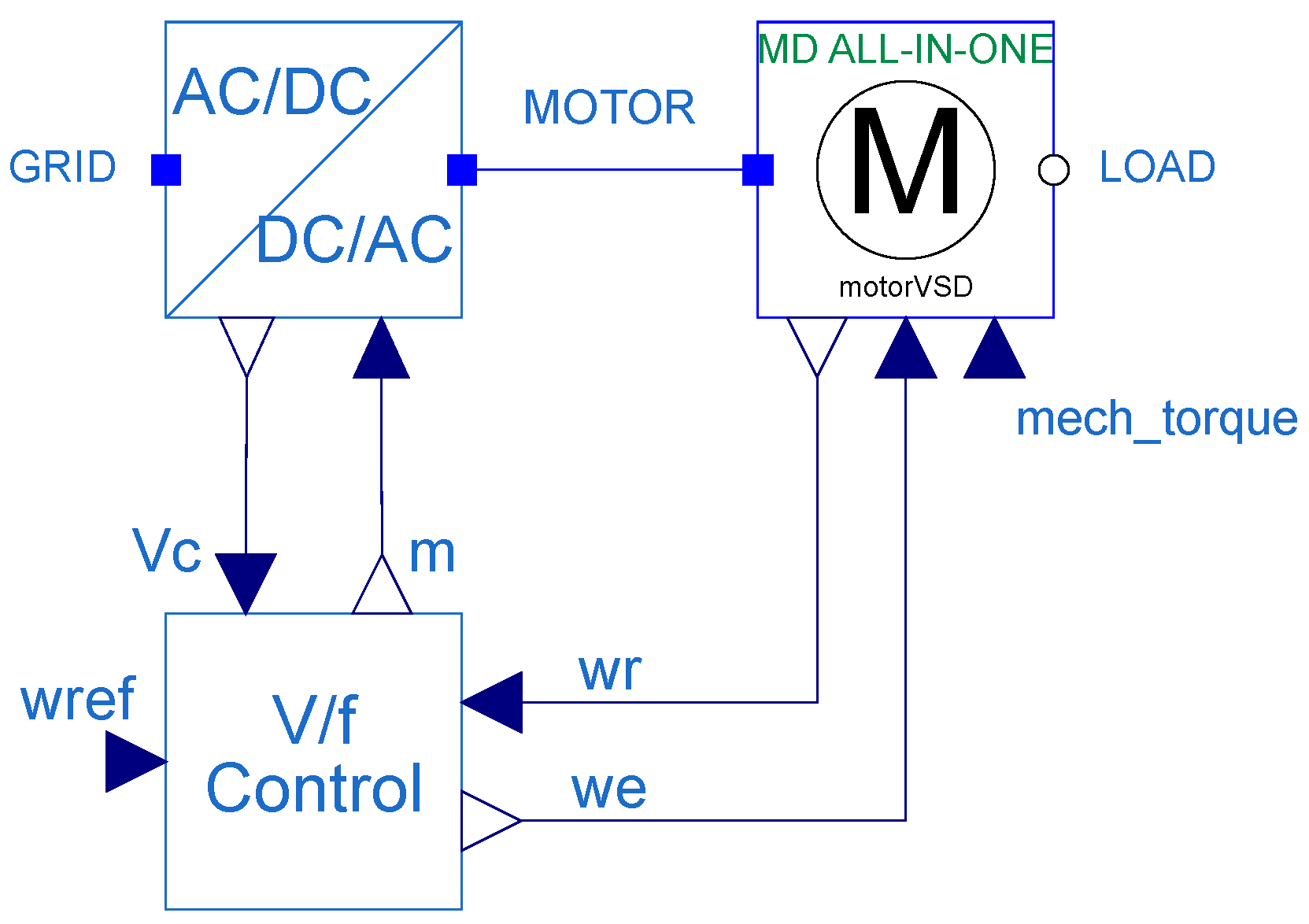
  • Motor setup: Parameter section that allows the user to select whether the motor is controllable and whether or not the motor will undergo startup. If Ctrl is true, then the motor can be controlled via an output signal that is fed to the we real input from Figure 1. If Ctrl is false, the motor is non-controllable, meaning that the motor’s impedance calculations are based on the nominal synchronous speed value defined inside the model. The parameter Sup defines the initial slip, when true, the motor rotor starts from the halt position, and false starts from the steady state.
  • Machine parameters: Parameter section where the user defines values for parameters that are ubiquitous to all motor models, which are the number of pairs of poles (N) and the rotor inertia (H).
  • Motor selection: Parameter section where the user defines the motor model for simulation. The drop-down item allows the user to choose between different models (MotorTypeI, MotorTypeIII, MotorTypeV, CIM5, and CIM6). The icon to the right of the drop-down option is the ‘Edit’ option, where the user can manually type the values of the parameters of the chosen induction motor model. For an example of a MotorTypeIII parametrization, refer to Appendix C.
The same model structure is present in the NonMultiDomainMotor, differentiating itself from the MultiDomainMotor by the lack of a flange connector; therefore, due to its modeling similarity, the explanation of the NonMultiDomainMotor model is omitted.

3.3. Single-Phase and Dual-Phase Induction Motor

Similar to how the MD and NMD three-phase induction motor models were developed, the single-phase induction motor (SPIM) and the dual-phase induction motor (DPIM) have a base class that allows for inheritance. One peculiarity of the SPIM is that due to the physical placement of the main stator poles, the resulting magnetic field pulsates instead of rotating, which is the case for the three-phase induction motor [33]. The consequence of having a pulsating magnetic field is that the motor will not rotate without an initial external torque applied to the rotor. Therefore, single-phase motors in real life include an auxiliary circuit that is switched on during the motor start process and is switched off once the motor reaches a user-defined rotational speed [27]. Due to this fact, single-phase motors can be modeled in two distinct ways: (a) steady-state operation, where the motor is assumed to be in a steady state and the startup process is neglected, and (b) full modeling of the main and auxiliary circuits, leading to the ability to simulate both startup and steady-state conditions. In this paper, when using the term “single-phase” motor models, the authors describe the steady-state representation of the motor, while the term “dual-phase” motor simply refers to the motor that can simulate both startup and steady-state operations. Because of the more complex circuit representation in the dual-phase motor model and because it can represent both steady-state and startup circuitry, the main focus in the following sections is to describe the DPIM motor model in the MD form.

3.3.1. Base Class for Multi-Domain and Non-Multi-Domain Models

The non-multi-domain and multi-domain base class applies to both SPIM and DPIM models, BaseNonMultiDomainSinglePhase and BaseMultiDomainSinglePhase, respectively, as shown in Figure 4.
The base class model for the SPIM and DPIM models, either MD or not, is very different from the structure shown for the base class of the three-phase induction motors. This is because the SPIM and DPIM induction motors have very few variables in common and, therefore, models derived from each base class will have different parameters and variables. The NMD base model is mainly comprised of power flow initialization parameters; therefore, all specific parameters and variables that describe each different model are expressed in the (derived) extended model. Figure 5 displays the diagram view of the MD base class model of the SPIM and DPIM models.
The difference between this class and the base class depicted in Figure 2 is the absence of the we, RealInput connector, and its aggregate components. The reason is that small machinery using these types of motors typically does not have variable speed drives connected to them, as they are generally used in applications requiring constant rotating speeds. The equation section of the MD base class model for the single-phase and dual-phase motors is shown below.
It is not surprising that Equations (1)–(3) from Listing 3 are identical to Equations (5)–(7) from Listing 1 since the interface follows the same structure on both models. The reader is directed to Section 3.1.1 for an explanation of the equation.
Listing 3. Modelica set of equations for the multi-domain single-phase and double-phase base class model.
 (1) - Rotor speed equation
ns = w_b;
nr = (1-s)*ns;
 
 (2) - Conversion from SI torqur to p.u. torque
Tmech_pu_sys = mech_torque/T_b;
Tmech_pu_motor = Tmech_pu_sys/CoB;
 
 (3) - Torque System base
T_b = S_b/w_b;

3.3.2. Creating Multi-Domain and Non-Multi-Domain Motor Models with Inheritance

The multi-domain DPIM extended motor model was developed to represent the startup and steady-state dynamics of the single-phase motor; to do so, the model required representation of both the main and auxiliary electrical winding circuits [27]. Due to the specific utility of the auxiliary winding, which involves generating a rotating electromagnetic torque during startup in single-phase motors, several different auxiliary winding circuit implementations are found in real-life single-phase motors. This paper will focus on describing two motor configurations, namely split-phase and capacitor-start single-phase motors (see Figure A1f,g in Appendix E). Split-phase motors have a modest starting torque and are used for applications that do not require high starting torques (fans, blowers, and centrifugal pumps). Meanwhile, capacitor-starter motors are more expensive, as they are implemented with an extra capacitor in the auxiliary winding for high starting torque capability (typically found in compressors, pumps, and air conditioners) [34]. Once the auxiliary winding circuit is disconnected, the single-phase motor operates under the magnetic field generated by the main winding, which is how the SPIM motor is modeled in the literature. For that reason, because of DPIM’s dual modeling capabilities, this section will focus on describing the Modelica equations that constitute the DPIM model. Listing 4 contains the set of complementary equations that uniquely defines the DPIM motor model, divided into twelve sections—three that are presented in Listing 3 and attributed by inheritance, and the reminder presented in Listing 4.
Listing 4. Modelica set of equations for the dual-phase multi-domain induction motor model.
 (4) - Reactance of the Capacitor, Main and Aux Winding
Xc = 1/(w_b*Cc);
Xmain = w_b*Lmain;
Xaux = w_b*Laux;
 
 (5) - Main and Aux Flux Linkage Coefficient Calculations
Kplus = (s*w_b)/(2*(Rr + j*s*w_b*Lr));
Kminus = (2 - s)*w_b/(2*(Rr + j*(2 - s)*w_b*Lr));
 
 (6) - Main and Aux Flux Linkage Calculations
Lambda_main = if s > switch_open_speed then (Lmain - j*Lmainr^2*(Kplus + Kminus))*Imain + 
   Lmainr*Lauxr*(Kplus - Kminus)*Iaux else (Lmain - j*Lmainr^2*(Kplus + Kminus))*Imain;
Lambda_aux = if s > switch_open_speed then - Lmainr*Lauxr*(Kplus - Kminus)*Imain + (Laux - 
   j*Lauxr^2*(Kplus + Kminus))*Iaux else 0*j;
 
 (7) - Main and Aux Winding Voltage
Vmain = V_b*(p.vr + j*p.vi);
Vaux = if sm > switch_open_speed then Vmain else 0*j;
 
 (8) - Main and Aux Winding Current
Imain = (Vmain - j*w_b*Lambda_main)/Rmain;
if sm > switch_open_speed and init == 1 then
Vaux = Iaux*Raux + j*w_b*Lambda_aux;
elseif sm > switch_open_speed and init == 2 then
Vaux = Iaux*Raux + j*w_b*Lambda_aux - j*Iaux/(w_b*Cc);
else
Iaux = 0*j;
end if;
 
 (9) - Conversion of calculated current to OpenIPSL connector current
p.ir = real(Imain + Iaux)/I_b;
p.ii = imag(Imain + Iaux)/I_b;
 
 (10) - Active and Reactive Power Calculation;
P = p.vr*p.ir + p.vi*p.ii;
Q = (-p.vr*p.ii) + p.vi*p.ir;
 
 (11) - Electromagnetic Torque Calculation
Te_pre = (Lmainr^2*Imain*conj(Imain) + Lauxr^2*Iaux*conj(Iaux))*conj(Kplus - Kminus) +
        j*Lmainr*Lauxr*(conj(Imain)*Iaux - Imain*conj(Iaux))*conj(Kplus + Kminus);
Te = (N/T_bm)*real(Te_pre);
 
 (12) - Mechanical Slip Equation
der(s) = (Tmech_pu_motor - Te)/(2*H);
  • Equation (4): Defines the reactance of the capacitor (Xc), the reactance of the main winding (Xmain), and the reactance of the auxiliary winding (Xaux). The parameter (Cc) is the auxiliary winding capacitance, the (Lmain) is the main winding inductance, and (Laux) is the auxiliary winding inductance.
  • Equation (5): Kplus and Kminus are coefficients that are used during the calculation of the electromagnetic torque.
  • Equation (6): Describes the flux linkage of the main (Lambda_main) and auxiliary (Lambda_aux) winding. Both flux linkage equations have if statements that are related to the auxiliary winding switching. During the startup process, the main winding circuit is parallel with the auxiliary winding circuit and the resulting flux linkage is different from when the main winding is the only circuit generating flux.
  • Equation (7): Defines the main and auxiliary winding complex voltage values. Once more, (Vaux), which is the auxiliary winding terminal voltage, has a different value during the startup and steady-state operations, determined by an if statement.
  • Equation (8): Defines the current through the main winding (Imain) and the auxiliary winding (Iaux). The reader will notice that there are two distinct equations for determining the (Iaux) value, related to the auxiliary winding configuration (decided as a parameter (init) that the user can choose).
  • Equation (9): Conversion of real and imaginary currents from ampere to per unit to comply with the pwpin OpenIPSL connector, instantiated as p.
  • Equation (10): Active (P) and reactive (Q) power calculation on the system base S_b.
  • Equation (11): Calculation of the electromagnetic torque (Te) generated by the DPIM motor model.
  • Equation (12): Describes the slip differential equation, representing the rate of change in the rotor speed as the motor drives a mechanical load. The slip is defined as the ratio between the mechanical and electromagnetic torque difference divided by double the motor’s inertia constant.

4. Variable Speed Drive Modeling

Conventional three-phase induction motors connected directly to the grid, once in a steady-state condition, operate at a single speed defined by the frequency of the grid’s voltage. However, in many industrial applications, one must control the motor’s speed and torque in order to fulfill a specific task, or with the overall goal of improving productivity and energy savings in pumps, fans, compressors, etc. Thus, induction motors are controlled via variable speed drives (VSDs), which are power electronic converters that enable the control of the motor’s terminal voltage magnitude or frequency. The power electronic interface of a standard VSD is shown in Figure 6.
The power electronic circuit of a VSD is typically built using a rectifier, a DC link circuit, an inverter, and its controller. The diode bridge (on the grid side) is composed of passive components, i.e., there is no means of controlling the diodes. However, the controllable side of the power electronic interface is on the thyristor bridge (on the motor side), where the frequency and angle of the AC motor voltage side are controlled through the switching of the thyristors. To reduce the simulation time required to represent the switching operations from the VSD power electronics interface, the authors chose to model the VSD power electronic interface in its “averaged” form. This representation provides an approximate “average response” that allows for much faster run times and avoids the problem of creating state events during simulation. Since the average model does not account for the switching component, the rectifier and inverter can be represented as shown in Figure 7.
The average rectified DC voltage V d o is defined as follows:
V d o = 3 2 π V s cos φ
where V s is the magnitude of the AC phasor voltage of the grid and φ is the angle of the diode rectifier ( φ = 0). The capacitor in the DC link circuit is responsible for holding a constant DC voltage, V c , during the steady state. The magnitude of the AC phasor voltage, V m , on the motor side, is modeled as a function of V c and a pulse width modulation (PWM) index, m. The phasor voltage on the motor side is as follows:
V m = 3 2 2 m V c
The motor voltage angle is chosen to be zero as it is the new reference to the motor and its magnitude depends on V c , the capacitor’s voltage, and the PWM modulation index.
The controllable parameter on the inverter side is the PWM index, which characterizes the amplitude modulation of the motor terminal voltage. Together with the voltage magnitude, the VSD controls the frequency of the motor terminal voltage, which automatically impacts the synchronous speed of the rotating magnetic field in the three-phase induction motor. The VSD control strategy that is the most common in industrial applications is scalar control, specifically the volts/hertz control. By increasing the motor terminal voltage and frequency at a constant ratio, it is possible to maintain an almost constant magnetic flux density in the motor air gap. Maintaining constant magnetic flux ensures constant electromagnetic torque in the motor, which is a desirable outcome. The volts/hertz logic diagram is shown in Figure 8.
The controller inputs are the green variables ω r (rotor speed) and ω r e f (synchronous reference speed), while the controller outputs are the blue variables m (PWM modulation index) and ω e (synchronous speed). The m output variable is limited in the range of 0 < m < 1 as the inverter can only modulate the voltage magnitude and not increase it above its nominal value. The limit to how much the synchronous speed can vary depends on the specific motor operation and is set through the limit values, w m a x and w m i n . The diagram view of the complete volts/hertz VSD model in Modelica is shown in Figure 9.
The reader will notice several common input and output variables between the block diagram in Figure 8 and the Modelica model in Figure 9. The sensed motor rotor speed, wr, which is an output in the MD motor model, is used as an input to the volts/hertz controller block, while an external angular reference (wref) determines the frequency/synchronous speed reference. The synchronous speed we and the PWM index m are calculated in the V/f control block, which is then used to control the magnitude and frequency of the voltage at the motor terminal. For more details on the modeling aspects of the Modelica ‘average’ VSD model from Figure 9, refer to [35].

5. Validation and Illustrative Results

To demonstrate the features of the developed models, the authors devised a set of simulations shown in this section. To verify that the results are consistent with the first-principles models/physics laws, we provide validation examples that test the behavior of the motor models. Furthermore, to present the innovative features suggested in this study, we offer illustrative examples. These examples encompass the operations of the variable speed drive (VSD) and multi-domain system models, incorporating the power grid, motor, and fluid domains.
The simulations are divided into five different categories:
  • Three-phase multi-domain motor validation example: Evaluates the performance of all the three-phase multi-domain motors compared to the reference simulation results from the Power System Toolbox (PST).
  • Three-phase non-multi-domain motor validation example: Evaluates the performance of the CIM5 NMD motor compared to the reference simulation results from Siemens PTI PSS® E.
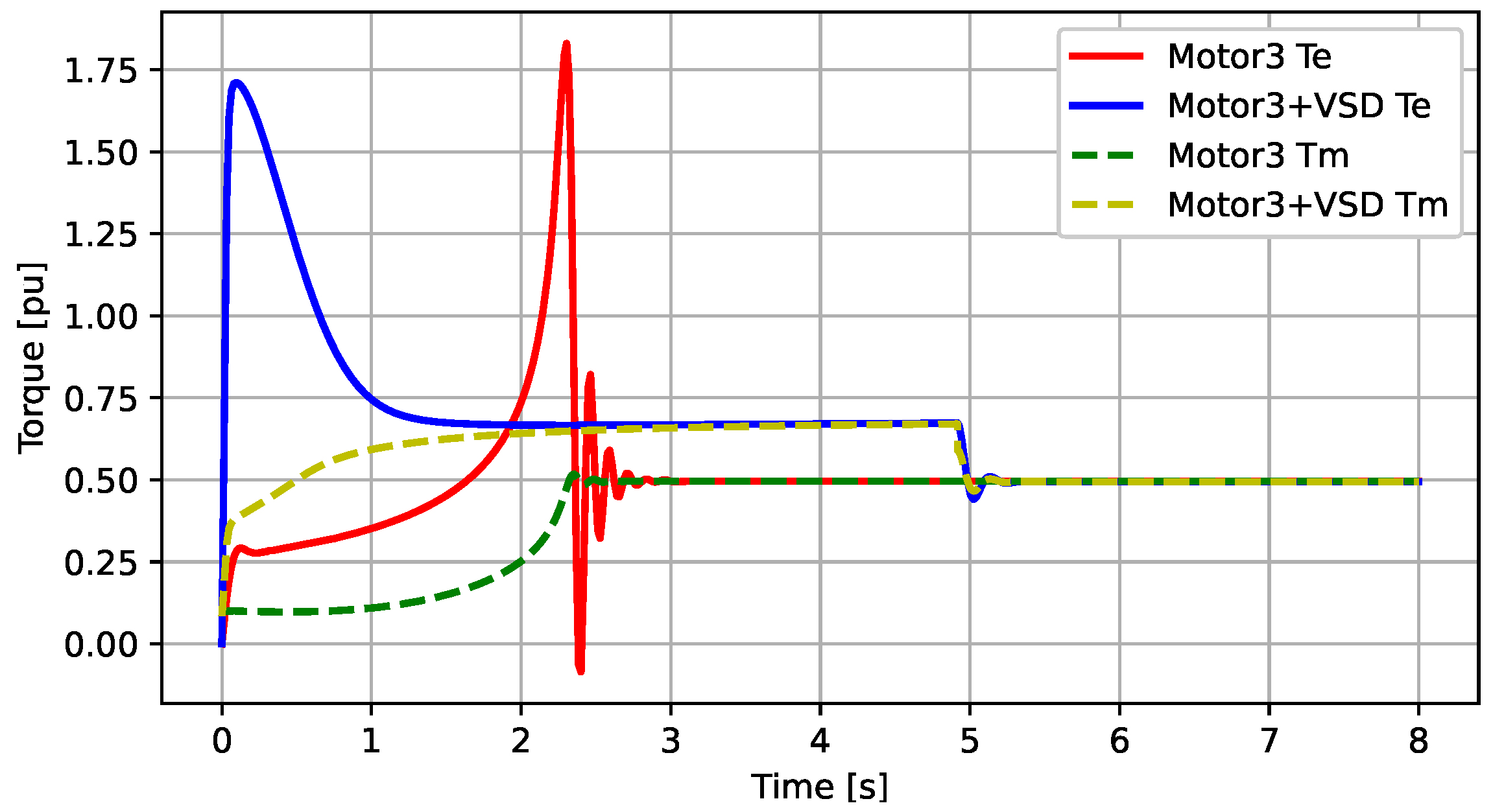
  • VSD-controlled motor startup example: Evaluates the performance of the VSD together with the three-phase MD motor for the case of a motor startup simulation.
  • Multi-domain SPIM and DPIM examples: Evaluates the performances of all MD variants of the single-phase induction motor (SPIM) and dual-phase induction motor (DPIM).
  • Multi-domain system application example: Demonstrates the capability of simulating multi-domain systems (power grid, multi-domain motor, and a fluidic system) in one holistic example.
  • Microgrid example with multiple generation units and load models: Demonstrates how the developed models can be integrated with a microgrid system example.
In all dynamic simulations exemplified in this section, we employ the DASSL solver (differential/algebraic system solver) [36]. This method is used for solving systems of differential-algebraic equations (DAEs). DASSL’s key strength is in functionally handling stiff systems of differential-algebraic equations, which are prevalent in dynamic power system simulations.

5.1. Three-Phase Multi-Domain Motor Validation Examples

To verify the accuracy of the three-phase MD induction motor models, we reproduced Example 11.7 from the book Power System Modeling, Computation, and Control by Chow et al. [37]. The authors of the book used the Power System Toolbox v3.0 (PST) [4], which is a MATLAB-based software, to perform a motor start simulation. The parameter values for the example are presented in Appendix B.
In the following study, we recreated the same system model as the one presented in [37], ensuring that all model parameters in the Modelica models matched precisely the reference models. The only modification made in both software environments was to use the infinite bus model to represent the grid. This adjustment was made to simplify the comparisons between the Modelica and PST-based models, i.e., to allow the excitation of the motor dynamics without any interference of other dynamic responses from other grid components. Figure 10 displays an example of the motor start in Modelica. No figure for the model in PST is available, as models in PST are defined through predefined data matrices and have no graphical schematic associated with them.
In Figure 10, the ALL-IN-ONE motor allows the user to simulate different MD three-phase motors simply by changing the selected motor model as a parameter. Meanwhile, the PST_Voltage, PST_Slip, PST_Pmotor, and PST_Qmotor components are lookup tables and are used to store the simulation results from PST to be used to compare with the Modelica model’s response. Figure 11 presents a comparison between active and reactive power consumption, highlighting distinct behavior in Motor1 when compared to the others. In Figure 11a, two noticeable oscillations in the active power consumption of Motor3, Motor5, CIM, and PST’s model, are observed: one at the beginning of the simulation and another around t = 2.35 s. The oscillation at t = 0 originates from the modeling assumption that the initial voltage behind the stator resistance R s is zero, i.e., e r e ( 0 ) = 0 and e i m ( 0 ) = 0 . Linearization of the non-linear equations at t = 0 reveals a pair of complex eigenvalues that are stable (with a negative real component) and exhibit an oscillation frequency of 60.0684  Hz, confirming the observed oscillation in Figure 11. Since the active and reactive power signals of the PST serve as our reference points for comparing multi-domain simulations, if the modified model can replicate the same response as the target value, we assume the correctness of the multi-domain model. However, as mentioned earlier, Motor1 does not incorporate the dynamics associated with the flux linkage in the motor rotor. Consequently, the output response of this model differs from the reference and its more detailed counterparts.
Figure 12 displays the initial slip values over time for all MD three-phase induction motors modeled using the ALL-IN-ONE motor component, including the reference simulation result generated from PST.
In the context of simulating the induction motor startup process, the slip is initialized at s = 1 when t = 0 (representing the motor starting from a halted condition). As the rotor speed increases, the slip progressively decreases until it reaches its steady-state value of s = 0.004 . Figure 12 clearly illustrates the distinctive behavior of Motor1 in comparison to other motors, especially as they approach their steady-state values. Note that Motor1 exhibits no oscillatory behavior at around t = 2.35 s due to its modeling assumptions. Unlike Motor3, Motor5, CIM, and PST’s model, Motor1 does not include the rotor cage modeling, resulting in the simplest possible three-phase induction motor model. As a result, it does not factor in fluctuations in the flux linkage within the rotor and stator coils. Motor1 is characterized by a single differential equation that describes the relationship between slip and torque, distinguishing it from the more detailed motor models. On the other hand, Motor3, Motor5, and CIM show similar results when compared to the reference model, confirming the validation process.
The results depicted in this subsection align with the characteristics observed in Example 11.7 of [37], simulated using the PST v3.0 software tool [4].

5.2. Three-Phase Non-Multi-Domain Motor Validation Example

Section 5.1 presents the validation procedure and results for the three-phase MD motor models, in which their responses are compared with those obtained from the PST software. Because the MD motor models implemented can be coupled to Modelica rotational components, the load torque expression is defined outside of the motor component. Siemens PTI PSS® E, on the other hand, has different induction motor models, where each model contains a different load torque expression built into it. The load torque equation from the validation example shown in Section 5.1 differs from the expression defined by the motor models CIM5 and CIM6 in PSS® E; therefore, this section is meant to compare the non-multi-domain motor models implemented against the reference software, PSS® E. To keep it concise, this section presents only the verification results that compare the implementation of the CIM5 model with PSS® E. The NMD CIM5 validation model is similar to the one presented in Figure 10; the sole difference is that there is no flange in the model and, thus, no mechanical interface components. For this reason, the graphical representation of the Modelica model is not shown in this section, although the parameter values for the validation example are presented in Appendix B. Figure 13 and Figure 14 show the active and reactive power consumption of the CIM5 motor model and its slip curve compared to the reference simulation obtained using PSS® E. Similar to the previous section, the results displayed here point to the accuracy of the induction motor model implemented in Modelica.

5.3. VSD-Controlled Motor Startup Example

In this example, a three-phase multi-domain motor model is simulated in two similar system models, as shown in Figure 15, where one model includes a VSD controller (top) and the second one does not (bottom). Observe that the power system is modeled using OpenIPSL components (components to the left of buses bus4_mt1 and bus4_mt2), followed by the components described in this paper. The system models were built based on Example 11.7 from [37], and the parameter values for the aforementioned example are presented in Appendix C.
The goal of this example is to show the impact of having a VSD on the motor startup process. The novelty shown in this example is the capability to vary the synchronous speed and terminal motor voltage in order to control the startup process, as well as having models that span multiple domains, which is not possible with power system simulation tools. The motor startup process involves gradually ramping up the synchronous speed and terminal voltage, resulting in reduced current draw from the motor during startup.
Figure 16 displays the current magnitude drawn by the Type III MD model connected to a VSD compared to the motor connected to the grid. For the sake of clarity in the plots, the authors show only one comparison example utilizing a Type III MD motor model. The red curve presents the current magnitude of the motor in the system without VSD, while the blue curve reflects the current magnitude of the motor in the system with VSD. The case with VSD displays a significantly smaller current magnitude during the startup process, which is set for 5 s. For this particular example, the voltage and synchronous speed increase at the same rate for a duration of 5 s until a peak voltage value of 1 p.u. and a frequency of 60 Hz (equivalent to achieving a synchronous speed of 2 π f rad/s). The spike in the blue torque curve demonstrates the transient response of the motor as the voltage and frequency increase, while the constant torque value after transient, from t = 1.5 s to t = 5 s, reflects the constant torque region of the motor with the variable voltage and variable frequency power supply. The red curve corresponds to the electromagnetic torque of the Type III motor connected to the grid with no VSD startup control. As expected, the VSD-driven motor experiences a constant torque during the startup process (after its initial transient), which is higher than the grid-connected motor. It is worth pointing out that the mechanical torque in both scenarios also changes; a higher initial motor torque from a halted position results in a counter-mechanical torque that is proportional to the applied force. For that reason, in Figure 17, the mechanical torque in the case with VSD (yellow dashed curve) is greater than the mechanical torque in the motor without VSD (green dashed curve).

5.4. Multi-Domain SPIM and DPIM Motor Model Validation Examples

In these examples, validation of the multi-domain SPIM and DPIM motor models is conducted through three different simulation scenarios that are designed to demonstrate the steady-state and startup operations of the SPIM and DPIM motor models.
As mentioned in Section 3.3, the SPIM motor model is intended to simulate post-startup scenarios, where the motor start process is not of interest and the user wants to initialize the simulation from its steady-state operation. To test the steady-state operation of the motor, the validation is carried out using the SPIM model, as shown in Figure 18, while the parameter values for this particular example are found in Appendix D.
This example is constructed in a way that the VariableTorque component will act like a ramp, linearly increasing the load torque applied to the motor until it reaches a new steady state condition. Figure 19 displays the result of the SPIM example simulation for a duration of 5 s. The red curve displays the electromagnetic torque of the SPIM model, while the blue curve displays the slip of the motor model. Initially, the plots of both curves in an interval of t = 0 to t = 1 start flat, which means that the simulation is initialized in a steady-state condition. From t = 1 to t = 4 s, the mechanical torque increases, and as such, the electromagnetic torque of the SPIM motor must increase to maintain the motor operation. Consequently, the slip also increases, which confirms that the motor under increasing loads has a reduction in the rotor speed. It is worth mentioning that in the circuit of Figure 18, the electrical system from the load_bus to the left represents one of the three phases of a three-phase electrical grid, which means that the model can emulate the operation of a single-phase induction motor in a single-phase electrical circuit common to North American households.
To test the startup dynamics of the single-phase induction motor, the validation is conducted utilizing the DPIM model. The model configuration closely resembles the one depicted in Figure 18, with the only distinction being the utilization of a DPIM motor model.
The developed DPIM model can model both a split-phase dual-phase and a capacitor-start dual-phase induction motor (their differences are highlighted in Section 3.3.2). Figure 20 displays the electromagnetic torque of the split-phase and capacitor-based startup configurations.
As expected, the capacitor-start DPIM motor is configured to experience a 90-degree shift between the main and auxiliary winding circuits, which consequently generates a higher startup torque versus the split-phase scheme. The black dashed curve displays the electromagnetic torque for the capacitor start, whereas the red solid curve represents the split-phase startup. In both cases, the auxiliary circuit is turned off once the slip reaches a predefined value of 0.1 [p.u.], in which case, the torque reduces to a value that the main stator winding can generate. It is worth mentioning that the results are consistent with the description in Chapter 9, Sections 9.2.1 and 9.2.2 of the book Electrical Machinery by Fitzgerald et al. [27].

5.5. Multi-Domain System Application Example

A simple yet illustrative example that demonstrates the capability of combining different libraries and creating a multi-domain system is shown in Figure 21.
The system model is configured to simulate an induction motor driving a mechanical pump that feeds water into a reservoir. This example, although very simple, can be used to mimic the fundamental functioning of a motor pumping water into a reservoir, similar to the pumping operation in a pumped storage hydro-power plant after its energy generation stage [38]. The component SOURCE is an infinite source of water, the pump component represents a centrifugal water pump, and the pipe and reservoir components represent the piping and water storage, correspondingly, inherited from the MSL Fluid library [39]. Another advantage of having such multi-domain models is the capability to analyze the impact of different contingencies (i.e., failures that deteriorate the system’s dynamic performance) in the different domains. For instance, the fault component simulates an electrical three-phase to ground fault, while the clogged_pipe valve component emulates an obstruction in a pipe. Figure 22a displays the active power and rotor speed for the Motor Type I case study during a 50 s simulation.
In this case study, the obstruction in the pipe starts to emerge at t = 25 s, clogging 90% of the pipe in 1 s. An electrical fault is set to occur at t = 35 s, for a duration of 0.3 s. The obstruction reduces the cross-section area of the pipe to 10%, increasing the load torque and, consequently, increasing the power drawn by the motor. The increase in power comes with a reduction in rotor speed (see the red curve in Figure 22a). Due to the electrical fault, the motor’s terminal voltage decreases, which consequently reduces the power drawn by the motor momentarily. Once the electrical fault is cleared, the motor returns to its previous state. Note that given the short electrical fault duration, there is no major impact on the hydraulic behavior (pipe mass flow and reservoir level). Thus, this example shows the value of expanding modeling capabilities beyond conventional scenarios common to power system tools.

5.6. Microgrid Example with Multiple Generation Units and Load Models

This example demonstrates how the developed models can be integrated with a microgrid. To model the grid, the OpenIPSL Library provides different generation sources, load models, and other component models, which together with the models developed in this manuscript, can be combined into a single and unified simulation model. In addition, we extend the model with a fluid sub-system, illustrating how the integrated model allows simulating the electrical, mechanical, and fluidic domains simultaneously within a single software environment.
The developed example is shown in Figure 23, representing a microgrid connected to the utility grid through a single point of common coupling (PCC).
The microgrid is represented by the system inside the green solid line, while the utility grid is represented by the system in the blue solid line. The microgrid consists of various generation units, including a combustion-based turbine-driven generator system, a photovoltaic (PV) plant, and a battery energy storage system (BESS) unit. The PV plant contains an irradiance-to-power block that allows to model of the variability of the injected DC going from PV cells/array. The synchronous generator is equipped with a primary-level control system comprising a speed governor and an automatic voltage regulator (AVR), while renewable sources have active and reactive power controls. All components responsible for energy production within the microgrid are categorized as distributed energy resources (DERs). DERs are small-scale energy sources typically located near the point of use or within the distribution network, with an energy production limit of 10 MW [40]. For this study, the synchronous generator in the microgrid has a capacity of 10 MW, while the rated active power of renewable energy sources is 5 MW. Lastly, the microgrid presents a mix of static and dynamic loads. The dynamic loads are a mix of the multi-domain motor and non-multi-domain motor models, including motor speed control with VSDs, which were presented in this paper. The static load represents the usual residential/commercial electrical loads.
The utility grid model includes a section of the power distribution system, a hydropower plant, and the remaining grid infrastructure. In this study, the synchronous generator serves as the primary energy source determining the voltage and frequency within the microgrid, while the renewable DERs function as “grid-following” components.
This example expands on the simulation capabilities demonstrated in the previous example from Section 5.5. It incorporates multiple motor philosophies, a grid, and a grid-connected microgrid into a single example. The static load includes a sinusoidal component, resulting in a sinusoidal variation in the active power consumption of the load.
In the context of motors, the non-multi-domain motors simulate a ventilation system, where one variable speed drive (VSD) controls the speed of three identical motors. In contrast, the multi-domain Type III motor represents a water pumping unit, which in this example could represent the water pumping station of a campus microgrid, for instance.
Overall, this example illustrates how—by using the developed models in this work—a user could now simulate multiple domains simultaneously.
In this example, the following sequence of events is applied to illustrate the model’s features, as follows:
  • Event 1: At t = 10 s, a reduction of 30% of the reference speed ω r e f of the VSD that controls the three non-multi-domain motors is applied. The reduction in ω r e f decreases both the motor terminal voltage magnitude and frequency, thus also reducing the power consumption.
  • Event 2: At t = 20 s, a reduction of 25% in the reference speed ω r e f of the VSD that controls the multi-domain motor is applied. Similar to Event 2, the multi-domain motor will also experience a reduction in power consumption.
  • Event 3: At t = 30 s, a reduction of 50% in irradiance levels (from 666.66 W / m 2 to 333.33 W / m 2 ) is applied to the solar PV plant. This results in a 50% reduction of the injected power from the PV generation unit.
  • Event 4: At t = 40 s, the circuit breaker tripping signal at the point of common coupling (PCC) is triggered, causing the microgrid to become isolated from the utility grid. Before isolation, the microgrid imported 3.3 MW of power from the utility, resulting in a power imbalance. Consequently, the overall frequency of the microgrid falls below the nominal value of 60 Hz during the islanding scenario.
Figure 24 showcases the simulation results for the microgrid system that withstood the four events detailed above.
When the microgrid becomes islanded at t = 40 s, the system loses approximately 4 MW of power from the utility grid (as seen in Figure 24a). The primary controllers of the microgrid generation units lack the capability of eliminating the frequency error (which is the task of the secondary level controller); thus, immediately after the circuit breaker trip, microgrid frequency displays a dip and reaches a new steady-state value of around 59.35 Hz (as seen in Figure 24e). Microgrid active power import is related to how much power the microgrid itself can generate; thus, at t = 30 s, when there is a reduction in irradiance levels, the amount of imported power must increase to balance power (as seen in Figure 24a). In Events 1 and 2, there is a reduction in the reference speed of the VSDs of all the induction motors involved in the simulation. The VSD reduces both the voltage magnitude and input frequency, leading to reduced power consumption (as seen in Figure 24b,c). Consequently, the pump operates at a reduced rotational speed and the mass flow in the water system is also reduced proportionally (as seen in Figure 24d).
These simulation results illustrate what is possible to study using multi-domain modeling, as enabled by the models developed in this paper, integrating them with models from the Modelica Standard Library and OpenIPSL.

6. Conclusions

This work presents the development, implementation, and validation of multi-domain and non-multi-domain three-phase and single-phase motor models that are voltage-/ frequency-controlled and, thus, can be coupled to a VSD model. The set of implemented motor models, along with the VSD, was developed to address a gap in traditional phasor domain power system modeling, enabling both rotational speed controllability over motor models as well as the ability to enrich the representation of the load processes coupled to the mechanical dynamics of the motor. Consequently, the new phasor domain motor models can now be coupled with detailed representations of the driven load, giving unique modeling capabilities that are unavailable in standard power system simulation tools, which only use a simplified torque equation to represent them. Simulation studies showed that the developed components are crucial for the detailed study of multi-domain systems, such as the electrical and hydraulic systems.

Author Contributions

Conceptualization, F.F., T.B. and L.V.; methodology, F.F. and L.V.; software, F.F., M.d.C. and L.V.; validation, F.F. and L.V.; formal analysis, F.F. and L.V.; investigation, F.F. and L.V.; resources, L.V.; writing—original draft preparation, F.F.; writing—review and editing, T.B., M.d.C. and L.V.; supervision, L.V.; project administration, L.V.; funding acquisition, L.V. All authors have read and agreed to the published version of the manuscript.

Funding

This research was funded by the U.S. Department of Energy’s Office of Energy Efficiency and Renewable Energy (EERE) under the Advanced Manufacturing Office, Award Number DE-EE0009139.

Data Availability Statement

The GitHub repository containing all the models and validation tests presented in this work can be found here: https://github.com/ALSETLab/OpenIMDML (accessed on 16 April 2024).

Acknowledgments

The authors would like to thank Abdul Rauf of the National Power Control Center, Islamabad, Pakistan, for assisting in conducting simulations to validate the implemented models against the PSS® E software. This paper was prepared as an account of work sponsored by an agency of the United States Government. Neither the United States Government nor any agency thereof, nor any of their employees, makes any warranty, express or implied, or assumes any legal liability or responsibility for the accuracy, completeness, or usefulness of any information, apparatus, product, or process disclosed, or represents that its use would not infringe privately owned rights. Reference herein to any specific commercial product, process, or service by trade name, trademark, manufacturer, or otherwise does not necessarily constitute or imply its endorsement, recommendation, or favoring by the United States Government or any agency thereof. The views and opinions of the authors expressed herein do not necessarily state or reflect those of the United States Government or any agency thereof.

Conflicts of Interest

Author Marcelo de Castro was employed by the company Mitsubishi Electric Power Products, Inc. The remaining authors declare that the research was conducted in the absence of any commercial or financial relationships that could be construed as a potential conflict of interest.

Abbreviations

The following abbreviations are used in this manuscript:
ACalternate current
CHPcombined heat and power
DCdirect current
DPIMdual-phase induction motor
GEGeneral Electric
MDmulti-domain
MSLModelica Standard Library
NMDnon-multi-domain
OpenIPSLOpen Instance Power System Library
PSATPower System Analysis Toolbox
PSTPower System Toolbox
VSDvariable speed drive
WECCWestern Electric Coordinating Council

Appendix A. Induction Motor Model Type III Parameters and Variables

  • w_sync: Synchronous speed variable toggled to either utilize the system nominal frequency parameter w_b or the input connection port we.
  • Ctrl: Boolean parameter that allows the user to choose between the controllable if Ctrl == true or non-controllable if Ctrl == false. If Ctrl == true, then motor impedance and motor frequency will vary based on an input value from the connector we, or else the motor frequency will be determined by w_b, which is the nominal system frequency in rad/s.
  • we: Modelica input connector for inputting the motor’s synchronous speed. In the case where Ctrl == false, the connector is eliminated from the model.
  • s: Induction motor slip, defined by the ratio between the difference in rotor and synchronous speeds to the synchronous speed of the rotating magnetic field. This variable is unitless.
  • w_b: Base frequency parameter, defined as w _ b = 2 π f n [rad/s], where f n = 60 [Hz].
  • Vr: Real component of the motor terminal voltage, expressed in per unit [p.u.], on the system base.
  • Vi: Imaginary component of the motor terminal voltage, expressed in per unit [p.u.], on the system base.
  • Ir: Real component of the motor consumed current, expressed in per unit [p.u.], on the system base.
  • Ii: Imaginary component of the motor consumed current, expressed in per unit [p.u.], on the system base.
  • pwpin: Ubiquitously used connector from OpenIPSL that contains four variables: two potential {pwpin.vr, pwpin.vi} and two flow {pwpin.ir, pwpin.ii} variables [41].
  • mech_torque: Mechanical torque in the Newton meter [N.m], which is both the input connector and a motor equation variable.
  • T_b: Base torque [N.m] of the system.
  • Tmech_pu_sys: Mechanical torque variable, expressed in per unit [p.u.], on the system base.
  • Tmech_pu_motor: Mechanical Torque variable, expressed in per unit [p.u.], on the motor base.
  • S_b: System apparent power base.
  • Xs: Stator winding impedance, expressed in per unit [p.u.], on the motor base.
  • Xm: Magnetization impedance, expressed in per unit [p.u.], on the motor base.
  • X1: Rotor winding impedance, expressed in per unit [p.u.], on the motor base.
  • X0: The sum of the stator impedance and the magnetization impedance, expressed in per unit [p.u.], on the motor base. In the case where Ctrl == false, the induction motor is not controllable and, thus, the impedance parameter is constant. If Ctrl == true, the induction motor is indeed controllable, and the impedance parameter is determined via the frequency ratio, w e X 0 w b .
  • Xp: The sum of the stator impedance and the parallel impedance Xm X 1 , expressed in per unit [p.u.], on the motor base. In the case where Ctrl == false, the induction motor is not controllable and, thus, the impedance parameter is constant. If Ctrl == true, the induction motor is indeed controllable, and the impedance parameter is determined via the frequency ratio, w e X p w b .
  • Tp0: Defines the open-circuit time constant of the induction motor [s]. In the case where Ctrl == false, the time constant is fixed, while if Ctrl == true, the induction motor time constant is determined via the frequency ratio, w e T p 0 w b .
  • epr: Real component of the voltage behind the stator resistance, r s , also known as the direct transient magnetization voltage.
  • epm: Imaginary component of the voltage behind the stator resistance, r s , also known as the quadrature transient magnetization voltage.

Appendix B. Non-Multi-Domain and Multi-Domain Motor Startup System Parameters

Table A1. Example Parameter Values.
ComponentParameterValueUnit
Inf1Machine Base (M_b)600MVA
Inertia (H)0s
Damping (D)0p.u.
Armature Resistance (R_a)0p.u.
d-axis reactance (X_d)0p.u.
bus1_mt1Base Voltage (V_b)16kV
Voltage Magnitude (V_0)1.05p.u.
Angle (angle_0)0°
bus2_mt1Base Voltage (V_b)230kV
Voltage Magnitude (V_0)1.03p.u.
Angle (angle_0)−6.739°
bus3_mt1Base Voltage (V_b)230kV
Voltage Magnitude (V_0)1.023p.u.
Angle (angle_0)−12.666°
bus4_mt1Base Voltage (V_b)23kV
Voltage Magnitude (V_0)1.015p.u.
Angle (angle_0)−12.882°
tf1_mt1Sending End Voltage (V_b)16kV
Voltage Rating (Vn)16kV
Resistance (rT)0p.u.
Reactance (xT)0.025p.u.
tf2_mt1Sending End Voltage (V_b)230kV
Voltage Rating (Vn)230kV
Resistance (rT)0p.u.
Reactance (xT)0.15p.u.
line_mt1Resistance (R)0p.u.
Reactance (X)0.02p.u.
Shunt Half Conductance (G)0p.u.
Shunt Half Susceptance (B)0p.u.
Load1Initial Active Power (P_0)500MW
Initial Reactive Power (Q_0)0Mvar
Voltage Magnitude (V_0)1.023p.u.
Angle (angle_0)−12.666°
Multi-Domain/Non-Multi-DomainMachine Base (M_b)15MVA
Number Pair Poles (N)1-
Inertia Constant (H)0.4s
Stator Resistance (Rs)0p.u.
Stator Reactance (Xs)0.0759p.u.
1st Cage Rotor Resistance (R1)0.0085p.u.
1st Cage Rotor Reactance (X1)0.0759p.u.
Magnetization Reactance (Xm)3.1241p.u.
load_inertia1Moment of Inertia (J)1kg · m 2
Torque EquationTorque (PST) 0.1 s + 0.5 ( 1 s ) 2 N · m
Torque (PSS® E) 0.534 ( 1 s ) 2 p.u. Machine Base
Synchronous_Speedsync_speed 2 π 60 rad/s

Appendix C. VSD-Controlled Motor Startup System Parameters

Table A2. Example Parameter Values.
ComponentParameterValueUnit
Inf1/Inf2Machine Base (M_b)600MVA
Inertia (H)0s
Damping (D)0p.u.
Armature Resistance (R_a)0p.u.
d-axis reactance (X_d)0p.u.
bus1_mt1/bus1_mt2Base Voltage (V_b)16kV
Voltage Magnitude (V_0)1.05p.u.
Angle (angle_0)0°
bus2_mt1/bus2_mt2Base Voltage (V_b)230kV
Voltage Magnitude (V_0)1.03p.u.
Angle (angle_0)−6.739°
bus3_mt1/bus3_mt2Base Voltage (V_b)230kV
Voltage Magnitude (V_0)1.023p.u.
Angle (angle_0)−12.666°
bus4_mt1/bus4_mt2Base Voltage (V_b)23kV
Voltage Magnitude (V_0)1.015p.u.
Angle (angle_0)−12.882°
tf1_mt1/tf1_mt2Sending End Voltage (V_b)16kV
Voltage Rating (Vn)16kV
Resistance (rT)0p.u.
Reactance (xT)0.025p.u.
tf2_mt1/tf2_mt2Sending End Voltage (V_b)230kV
Voltage Rating (Vn)230kV
Resistance (rT)0p.u.
Reactance (xT)0.15p.u.
line_mt1/line_mt2Resistance (R)0p.u.
Reactance (X)0.02p.u.
Shunt Half Conductance (G)0p.u.
Shunt Half Susceptance (B)0p.u.
Load1/Load2Initial Active Power (P_0)500MW
Initial Reactive Power (Q_0)0Mvar
Voltage Magnitude (V_0)1.023p.u.
Angle (angle_0)−12.666°
motor/motorVSDMachine Base (M_b)15MVA
Number Pair Poles (N)1-
Inertia Constant (H)0.4s
Stator Resistance (Rs)0p.u.
Stator Reactance (Xs)0.0759p.u.
1st Cage Rotor Resistance (R1)0.0085p.u.
1st Cage Rotor Reactance (X1)0.0759p.u.
Magnetization Reactance (Xm)3.1241p.u.
load_inertia1/load_inertia2Moment of Inertia (J)1kg · m 2
Torque_EquationTorq 0.1 s + 0.5 ( 1 s ) 2 N · m
TorqVSD 0.1 s + 0.5 ( 1 s ) 2 N · m
Synchronous_Speedsync_speed 2 π 60 rad/s

Appendix D. SPIM/DPIM Validation Example System Parameters

Table A3. Example Parameter Value.
ComponentParameterValueUnit
InfMachine Base (M_b)100MVA
Inertia (H)0s
Damping (D)0p.u.
Armature Resistance (R_a)0p.u.
d-axis reactance (X_d)0p.u.
inf_busBase Voltage (V_b)230V
Voltage Magnitude (V_0)1.0p.u.
Angle (angle_0)0°
load_busBase Voltage (V_b)230V
Voltage Magnitude (V_0)0.999p.u.
Angle (angle_0)0.016°
SPIMMachine Base (M_b)3.5kVA
Base Voltage (V_b)230V
Number Pair Poles (N)1-
Inertia Constant (H)0.1s
Stator Winding Resistance (R1)0.01p.u.
Rotor Winding Resistance (R2)0.05p.u.
Stator Winding Reactance (X1)0.01p.u.
Rotor Winding Reactance (X2)0.01p.u.
Magnetization Reactance (Xm)0.1p.u.
DPIMMachine Base (M_b)3.5kVA
Base Voltage (V_b)230V
Number Pair Poles (N)1-
Inertia Constant (H)0.1s
Aux Winding cut-off speed (switch_open_speed)0.1-
Mutual-inductance of the main winding (Lmainr)0.6mH
Self-inductance of the magnetizing branch (Lmain)0.0860H
Mutual-inductance of the auxiliary winding (Lauxr)0.9mH
Self-inductance of the auxiliary winding (Laux)0.1960H
Self-inductance of the equivalent rotor windings (Lr)4.7 μ H
Resistance of the main winding (Rmain)0.58 Ω
Resistance of the rotor winding (Rr)0.0376m Ω
Resistance of the auxiliary winding (Raux)3.37 Ω
Capacitance of the capacitor-start (Cc)0.3mF
load_inertiaMoment of Inertia (J)0.1kg · m 2
VariableTorqueInitialTorque0.041p.u.
FinalTorque0.649p.u.
startTime1s
duration3s

Appendix E. Induction Motor Steady-State Model Diagrams

Figure A1. Electrical circuit for different induction motor models. (a) Electrical circuit for the PSAT-based three-phase induction motor type I. (b) Electrical circuit for the PSAT-based three-phase induction motor type III. (c) Electrical circuit for the PSAT-based three-phase induction motor type V, PSS® E CIM5, and CIM6 Type (A). (d) Electrical Circuit for the three-phase PSS® E CIM5, and CIM6 Type (B). (e) Electrical circuit for the single-phase induction motor. (f) Electrical Circuit for the split-phase dual-phase induction motor. (g) Electrical circuit for the capacitor-start dual-phase induction motor.
Electronics 13 01614 g0a1

References

  1. Electric, G. GE Successfully Completed the No-Load Testing of One of the World’s Largest 80-Megawatt Induction Motors for the LNG Industry. 2024. Available online: https://www.gepowerconversion.com/news/ge-successfully-completed-no-load-testing-one-worlds-largest-80-megawatt-induction (accessed on 16 April 2024).
  2. IEEE Standard 399; Recommended Practice for Industrial and Commercial Power Systems Analysis. IEEE: Piscataway. NJ, USA, 1997.
  3. Siemens PTI. PSS®E 34.2.0 Model Library; Siemens Power Technologies International: Schenectady, NY, USA, 2017. [Google Scholar]
  4. Chow, J.H.; Cheung, K.W. A toolbox for power system dynamics and control engineering education and research. IEEE Trans. Power Syst. 1992, 7, 1559–1564. [Google Scholar] [CrossRef]
  5. Milano, F.; Vanfretti, L.; Morataya, J.C. An open source power system virtual laboratory: The PSAT case and experience. IEEE Trans. Educ. 2008, 51, 17–23. [Google Scholar] [CrossRef]
  6. Overbye, T.J.; Sauer, P.W.; Marzinzik, C.M.; Gross, G. A user-friendly simulation program for teaching power system operations. IEEE Trans. Power Syst. 1995, 10, 1725–1733. [Google Scholar] [CrossRef]
  7. Manual, P.U. PSLF Version 18.1 _01. 18th ed. 2020. Available online: https://www.gevernova.com/consulting/software/pslf (accessed on 18 February 2022).
  8. Milano, F. Power System Modelling and Scripting; Springer Science & Business Media: Berlin/Heidelberg, Germany, 2010. [Google Scholar]
  9. Neukomm, M.; Nubbe, V.; Fares, R. Grid-Interactive Efficient Buildings Technical Report Series: Overview of Research Challenges and Gaps; Tech. Rep. DOE/GO-102019-5227; DOE: Washington, DC, USA, 2019.
  10. Kosterev, D.; Meklin, A.; Undrill, J.; Lesieutre, B.; Price, W.; Chassin, D.; Bravo, R.; Yang, S. Load modeling in power system studies: WECC progress update. In Proceedings of the 2008 IEEE PES GM, Pittsburgh, PA, USA, 20–24 July 2008; pp. 1–8. [Google Scholar]
  11. Ma, Z.; Wang, Z.; Wang, Y.; Diao, R.; Shi, D. Mathematical representation of WECC composite load model. J. Mod. Power Syst. Clean Energy 2020, 8, 1015–1023. [Google Scholar] [CrossRef]
  12. US Department of Energy. Combined heat and power technology fact sheet series. Reciprocating Engines 2016, 1123, 1–5. [Google Scholar]
  13. Schweiger, G.; Gomes, C.; Engel, G.; Hafner, I.; Schoeggl, J.; Posch, A.; Nouidui, T. An empirical survey on co-simulation: Promising standards, challenges and research needs. Simul. Model. Pract. Theory 2019, 95, 148–163. [Google Scholar] [CrossRef]
  14. Jorissen, F.; Wetter, M.; Helsen, L. Simulation Speed Analysis and Improvements of Modelica Models for Building Energy Simulation. In Proceedings of the 11th International Modelica Conference, Versailles, France, 21–23 September 2015; pp. 59–69. [Google Scholar]
  15. Braun, W.; Casella, F.; Bachmann, B. Solving Large-scale Modelica Models: New Approaches and Experimental Results using OpenModelica. In Proceedings of the 12th International Modelica Conference, Prague, Czech Republic, 15–17 May 2017; pp. 557–563. [Google Scholar]
  16. Henningsson, E.; Olsson, H.; Vanfretti, L. DAE Solvers for Large-Scale Hybrid Models. In Proceedings of the 13th International Modelica Conference, Regensburg, Germany, 4–6 March 2019; p. 12. [Google Scholar]
  17. US Department of Energy. Improving Motor and Drive System Performance: A Sourcebook for Industry; US Department of Energy: Washington, DC, USA, 2014.
  18. Nyserda. Put Energy to Work. 2024. Available online: https://www.nyserda.ny.gov/PutEnergyToWork/Energy-Program-and-Incentives/Industrial-and-Special-Equipment-Programs-and-Incentives (accessed on 16 April 2024).
  19. Fritzson, P. Principles of Object-Oriented Modeling and Simulation with Modelica 3.3: A Cyber-Physical Approach; John Wiley & Sons: Hoboken, NJ, USA, 2014. [Google Scholar]
  20. de Castro, M.; Winkler, D.; Laera, G.; Vanfretti, L.; Dorado-Rojas, S.A.; Rabuzin, T.; Mukherjee, B.; Navarro, M. Version [OpenIPSL 2.0. 0]-[iTesla Power Systems Library (iPSL): A Modelica library for phasor time-domain simulations]. SoftwareX 2023, 21, 101277. [Google Scholar] [CrossRef]
  21. Fritzson, P.; Engelson, V. Modelica—A unified object-oriented language for system modeling and simulation. In Proceedings of the European Conference on Object-Oriented Programming; Springer: Berlin/Heidelberg, Germany, 1998; pp. 67–90. [Google Scholar]
  22. Fachini, F.; Castro, M.d.; Bogodorova, T.; Vanfretti, L. OpenIMDML: Open Instance Multi-Domain Motor Library utilizing the Modelica modeling language. SoftwareX 2023, 24, 101591. [Google Scholar] [CrossRef]
  23. Brück, D.; Elmqvist, H.; Mattsson, S.E.; Olsson, H. Dymola for multi-engineering modeling and simulation. In Proceedings of the 2nd International Modelica Conference, Oberpfaffenhofen, Germany, 18–19 March 2022; Volume 2002, pp. 55-1–55-8. [Google Scholar]
  24. Fritzson, P.; Aronsson, P.; Lundvall, H.; Nyström, K.; Pop, A.; Saldamli, L.; Broman, D. The OpenModelica modeling, simulation, and development environment. In Proceedings of the 46th Conference on Simulation and Modelling of the Scandinavian Simulation Society (SIMS2005), Trondheim, Norway, 13–14 October 2005. [Google Scholar]
  25. Saidur, R. A review on electrical motors energy use and energy savings. Renew. Sustain. Energy Rev. 2010, 14, 877–898. [Google Scholar] [CrossRef]
  26. Mattsson, S.E.; Elmqvist, H.; Otter, M. Physical system modeling with Modelica. Control Eng. Pract. 1998, 6, 501–510. [Google Scholar] [CrossRef]
  27. Fitzgerald, A.E.; Kingsley, C.; Umans, S.D.; James, B. Electric Machinery; McGRAW-Hill: New York, NY, USA, 2003; Volume 5. [Google Scholar]
  28. Milano, F. An open source power system analysis toolbox. IEEE Trans. Power Syst. 2005, 20, 1199–1206. [Google Scholar] [CrossRef]
  29. Pelchen, C.; Schweiger, C.; Otter, M. Modeling and simulating the efficiency of gearboxes and of planetary gearboxes. In Proceedings of the 2nd International Modelica Conference, Oberpfaffenhofen, Germany, 18–19 March 2022; pp. 257–266. [Google Scholar]
  30. Vanfretti, L.; Rabuzin, T.; Baudette, M.; Murad, M. iTesla Power Systems Library (iPSL): A Modelica library for phasor time-domain simulations. SoftwareX 2016, 5, 84–88. [Google Scholar] [CrossRef]
  31. Tiller, M. Introduction to Physical Modeling with MODELICA; Springer Science & Business Media: Berlin/Heidelberg, Germany, 2012; Volume 615. [Google Scholar]
  32. Monticelli, A.J. Load Flow in Electric Power Networks; Edgard Blucher: Sao Paulo, SP, Brazil, 1983. (In Portuguese) [Google Scholar]
  33. Ong, C.M. Dynamic Simulation of Electric Machinery: Using MATLAB/SIMULINK; Prentice Hall PTR: Upper Saddle River, NJ, USA, 1998; Volume 5. [Google Scholar]
  34. Chapman, S.J. Electric Machinery Fundamentals; McGraw-Hill: New York, NY, USA, 2004. [Google Scholar]
  35. Fachini, F.; De Castro, M.; Liu, M.; Bogodorova, T.; Vanfretti, L.; Zuo, W. Multi-Domain Power and Thermo-Fluid System Stability Modeling using Modelica and OpenIPSL. In Proceedings of the 2022 IEEE Power & Energy Society General Meeting (PESGM), Denver, CO, USA, 17–21 July 2022; pp. 1–5. [Google Scholar]
  36. Petzold, L.R. Description of DASSL: A Differential/Algebraic System Solver; Technical Report; Sandia National Labs: Livermore, CA, USA, 1982. [Google Scholar]
  37. Chow, J.H.; Sanchez-Gasca, J.J. Power System Modeling, Computation, and Control; John Wiley & Sons: Hoboken, NJ, USA, 2020. [Google Scholar]
  38. Rehman, S.; Al-Hadhrami, L.M.; Alam, M.M. Pumped hydro energy storage system: A technological review. Renew. Sustain. Energy Rev. 2015, 44, 586–598. [Google Scholar] [CrossRef]
  39. Franke, R. Standardization of thermo-fluid modeling in Modelica Fluid. In Proceedings of the 7th Modelica Conference, Como, Italy, 20–22 September 2009; pp. 1–10. [Google Scholar]
  40. US. Department of Energy, Federal Energy Management Program. Using Distributed Energy Resources-A How-to Guide for Federal Energy Managers. Cogener. Compet. Power J. 2002, 17, 37–68. [Google Scholar]
  41. Baudette, M.; Castro, M.; Rabuzin, T.; Lavenius, J.; Bogodorova, T.; Vanfretti, L. OpenIPSL: Open-instance power system library—Update 1.5 to “iTesla power systems library (iPSL): A modelica library for phasor time-domain simulations”. SoftwareX 2018, 7, 34–36. [Google Scholar] [CrossRef]
Figure 1. Icon view of the (a) non-multi-domain base class model; (b) multi-domain base class model.
Electronics 13 01614 g001
Figure 2. Diagram view of the multi-domain base class model for three-phase induction motors.
Electronics 13 01614 g002
Figure 3. All-in-one MultiDomainMotor parameter selection screen.
Electronics 13 01614 g003
Figure 4. Icon view of the (a) non-multi-domain base class model; (b) multi-domain base class model.
Electronics 13 01614 g004
Figure 5. Diagram view of the multi-domain base class model for single-phase and dual-phase induction motors.
Electronics 13 01614 g005
Figure 6. Typical VSD three-phase power electronic circuit.
Electronics 13 01614 g006
Figure 7. Typical VSD three-phase average power electronic circuit.
Electronics 13 01614 g007
Figure 8. Closed−loop volts/hertz control diagram.
Electronics 13 01614 g008
Figure 9. Diagram view of a complete VSD model.
Electronics 13 01614 g009
Figure 10. Multi-domain induction motor validation example.
Electronics 13 01614 g010
Figure 11. Comparison between the induction motor simulation results and the PST reference: (a) active power; (b) reactive power.
Electronics 13 01614 g011
Figure 12. Comparison between the induction motor slip values and the PST reference.
Electronics 13 01614 g012
Figure 13. Comparison between the induction motor simulation results and PSS® E reference: (a) active power; (b) reactive power.
Electronics 13 01614 g013
Figure 14. Comparison between the induction motor slip values and the PSS® E reference.
Electronics 13 01614 g014
Figure 15. VSD startup multi-domain induction motor comparison example.
Electronics 13 01614 g015
Figure 16. Startup current comparison.
Electronics 13 01614 g016
Figure 17. Mechanical and electromagnetic torque comparison.
Electronics 13 01614 g017
Figure 18. Multi-domain SPIM model validation example.
Electronics 13 01614 g018
Figure 19. SPIM electromagnetic torque (Te) and slip characteristics.
Electronics 13 01614 g019
Figure 20. Electromagnetic torque versus slip for the split-phase and capacitor-start DPIM motor.
Electronics 13 01614 g020
Figure 21. Multi-domain example that comprises OpenIPSL, newly developed components, and MSL Fluid components.
Electronics 13 01614 g021
Figure 22. Simulation results: (a) motor active power and rotor speed; (b) load reservoir level and pipe mass flow.
Electronics 13 01614 g022
Figure 23. Microgrid system example with multiple generation units and multiple load sources.
Electronics 13 01614 g023
Figure 24. Simulation results: (a) microgrid active power import; (b) total active power consumption from the three non-multi-domain induction motors; (c) total active power consumption of the multi-domain motor; (d) water system mass flow rate; (e) microgrid frequency.
Electronics 13 01614 g024aElectronics 13 01614 g024b
Disclaimer/Publisher’s Note: The statements, opinions and data contained in all publications are solely those of the individual author(s) and contributor(s) and not of MDPI and/or the editor(s). MDPI and/or the editor(s) disclaim responsibility for any injury to people or property resulting from any ideas, methods, instructions or products referred to in the content.

