
Research on 3D Visualization of Drone Scenes Based on Neural Radiance Fields
1
State Key Laboratory of Resources and Environmental Information System, Institute of Geographic Sciences and Natural Resources Research, Chinese Academy of Sciences, Beijing 100101, China
2
College of Resource and Environment, University of Chinese Academy of Sciences, Beijing 100049, China
*
Author to whom correspondence should be addressed.
Electronics 2024, 13(9), 1682; https://doi.org/10.3390/electronics13091682
Submission received: 3 April 2024
/
Revised: 20 April 2024
/
Accepted: 25 April 2024
/
Published: 26 April 2024
(This article belongs to the Special Issue Advances in Computer Vision and Deep Learning and Its Applications)
Abstract
:Neural Radiance Fields (NeRFs), as an innovative method employing neural networks for the implicit representation of 3D scenes, have been able to synthesize images from arbitrary viewpoints and successfully apply them to the visualization of objects and room-level scenes (<50 m2). However, due to the capacity limitations of neural networks, the rendering of drone-captured scenes (>10,000 m2) often appears blurry and lacks detail. Merely increasing the model’s capacity or the number of sample points can significantly raise training costs. Existing space contraction methods, designed for forward-facing trajectory or the 360° object-centric trajectory, are not suitable for the unique trajectories of drone footage. Furthermore, anomalies and cloud fog artifacts, resulting from complex lighting conditions and sparse data acquisition, can significantly degrade the quality of rendering. To address these challenges, we propose a framework specifically designed for drone-captured scenes. Within this framework, while using a feature grid and multi-layer perceptron (MLP) to jointly represent 3D scenes, we introduce a Space Boundary Compression method and a Ground-Optimized Sampling strategy to streamline spatial structure and enhance sampling performance. Moreover, we propose an anti-aliasing neural rendering model based on Cluster Sampling and Integrated Hash Encoding to optimize distant details and incorporate an L1 norm penalty for outliers, as well as entropy regularization loss to reduce fluffy artifacts. To verify the effectiveness of the algorithm, experiments were conducted on four drone-captured scenes. The results show that, with only a single GPU and less than two hours of training time, photorealistic visualization can be achieved, significantly improving upon the performance of the existing NeRF approaches.
1. Introduction
In recent years, neural network-driven implicit representation methods [1,2,3,4,5] have demonstrated exceptional performance in applications such as high-precision 3D reconstruction, thereby attracting extensive attention from researchers in the field of computer graphics. This approach takes the coordinates of a spatial point as input to predict the attributes of an object at that point. Compared to traditional explicit representation methods (such as point clouds, voxels, and meshes), the neural network-based implicit representation allows for the fine sampling of 3D objects at any spatial resolution. This results in the seamless reconstruction of scenes with rich geometric texture details and realistic visual effects that better meet the demands for authenticity.
One of the most notable works in this area are Neural Radiance Fields (NeRFs) [6]. NeRFs achieve an end-to-end process of scene modeling and rendering, enabling highly realistic reconstructions of scenes from just a set of multi-view photos, and allowing the viewing of 3D scenes from arbitrary angles. This method has developed rapidly in recent years and has broken through the limitations of explicit data structures in previous 3D surface models, with a particular focus on enhancing the ability to capture the details of real scenes. It is characterized by a high degree of automation, efficient training and rendering processes, and high fidelity in rendering effects. Notably, it addresses common issues in photogrammetry such as texture distortion and loss. Despite drawbacks such as significant computational demand and insufficient geometric precision, the technology is continually being optimized and has shown immense potential for application in various fields, including virtual reality (VR) and augmented reality (AR) [7], autonomous driving [8], robotic vision [9], large-scale scene generation [10], and film production [11].
While NeRFs and their derivative algorithms have shown their potential as powerful and easily optimizable 3D scene visualization algorithms, they face significant challenges when dealing with scenes captured by drones. For open scenes, the vanilla NeRF compresses the forward-unbounded scenes into a unit cube, while Mip-NeRF 360 [12] encapsulates 360-degree unbounded scenes within a bounded spherical space. However, these two methods of spatial compression are only suitable for camera trajectories that are either fixed in orientation or rotate 360 degrees, and not for the multi-loop circling shots typical of drones. Furthermore, to precisely locate surfaces in larger scenes, NeRFs needs to sample more points along the light ray. Although DoNeRF [13] and Mip-NeRF 360 [12] have optimized the distribution of sampling points through improved sampling functions, they tend to concentrate points near the camera, whereas the areas of interest in drone scenes are often at a distance. Under outdoor open scenes, NeRFs are constrained by model complexity, as capturing and expressing the full information contained in drone scenes requires a larger neural network and more GPU memory. Mega-NeRF [14] uses multiple neural networks to represent different aspects of the scene, but this demands significant computational resources, necessitating several GPUs working continuously for days or even weeks. DVGO, Plenoxels, TensoRF, and Instant-NGP [15,16,17,18] introduce feature grids to simplify the neural network architecture, significantly improving training and inference speeds, but this may lead to speckle noise during visualization. In drone scenes, the spatial area covered by a single pixel increases significantly with distance from the camera. Mip-NeRF [19] encodes LOD (Levels of Detail)-like information into the neural network’s input, allowing the model to dynamically adjust rendering precision based on the distance between observer and object, but the training cost for this method is high and the speed is slow. Moreover, complex lighting variations and sparse data capture in outdoor scenes can cause outliers and fog artifacts, further affecting rendering quality. Faced with these challenges, this paper seeks to address the following question: How can we achieve higher-quality visualization of drone scenes with limited computational resources and relatively fast convergence speed?
Considering the shortcomings of existing NeRF methods in drone-captured scenes, we introduce a NeRF framework specifically designed for the 3D visualization of drone scenes. The framework incorporates multi-resolution hash grids [18], which store features directly in a hash table to obtain prior information about the scene and alleviate the computational burden on the neural network, thus overcoming the high computational cost and long training time associated with the vanilla NeRF model. Our major contributions can be summarized as follows:
- We introduce a novel spatial compression technology to specifically address the multi-circle surround top-down flight paths performed by drones, and to integrate it with an efficient drone scene sampling method to significantly reduce the number of sampling points and enhance the performance of NeRFs;
- We combine the speed advantages of the feature grid-based approach with methods that maintain quality at a distant scale to accelerate the training process and effectively eliminate aliasing in long-range views, thereby enhancing the rendering quality when observed from a distance;
- Under the constraints of using only drone imagery as the data source and limited computational resources, we have realized the rapid convergence of the radiance field and improved the visual quality of drone-scene visualizations.
2. Related Work
The classic Neural Radiance Fields (NeRFs) paper [6] has sparked a plethora of subsequent research endeavors. We will discuss several approaches from a non-exhaustive list that pertain to aspects relevant to our work.
2.1. NeRFs for Sample Strategy Improvement
The hierarchical volume sampling technique introduced by the vanilla NeRF has made a significant impact on enhancing sampling outcomes. Further research has continued to refine this sampling method from a variety of perspectives. “NeRF in detail” [20] optimizes sample collection in NeRFs with a differentiable module, enhancing training and outperforming the vanilla model in view synthesis quality while lowering computational costs. NeuSample [21] accelerates rendering by substituting NeRFs’ coarse sampling with a neural sample field without sacrificing quality. DONeRF [13] reduces needed samples with a logarithmic strategy and depth priors. AdaNeRF [22] achieves real-time rendering with an innovative dual network that improves sampling efficiency. Enerf [23] boosts rendering speed with a depth-guided sampling that relies on predicted coarse geometry. TermiNeRF [24] efficiently maps camera rays to influential ray positions, streamlining neural-field model rendering and training. In this paper, we have adopted a simple yet effective sampling strategy that is particularly suited to drone-captured scenes.
2.2. Unbounded Scenes NeRFs
Generally, NeRF models are confined to encoding bounded scenes. To extend their application to unbounded scenes, current research has introduced a series of spatial contraction techniques. NeRF++ [25] introduces an “inverted sphere parametrization” to map unbounded scenes into a finite space by separating foreground and background into different coordinate systems. Mip-NeRF 360 [12] by Barron et al. maps infinite spherical spaces into bounded ones for unbounded scene rendering. MeRF [26] offers a contraction function for real-time large-scale rendering, maintaining linearity within a bounded space. Nerfstudio [27] adopts an L∞ norm to compress into a cubic space, enhancing compatibility with voxel-based encoding and addressing discontinuities present in other methods. ImmersiveNeRF [28] proposes a novel foreground–background hybrid representation, focusing on unbounded scenes captured from an inside-out configuration. MMPI [29] and Nex360 [30] expand MPI representation for complex scene synthesis from multiple perspectives. We have utilized an intuitive and efficient spatial contraction approach that is particularly well-suited for handling drone-captured surround top–down trajectories.
2.3. Large-Scale Scene NeRFs
The vanilla NeRF framework was designed primarily for small-scale scenes or objects. However, extending a NeRF to handle large-scale scenes would greatly expand its range of applications. A mega-NeRF [14] partitions the scene into segments and employs a sub-NeRF to implicitly represent each block. A block-NeRF [10] reconstructs urban-scale scenes from street-view images, using appearance embeddings and dynamic composition of NeRF blocks for neural rendering. Switch-NeRF [31] employs a gating network for scene decomposition and assigns points to various NeRF subnetworks for efficient large-scale reconstruction. Urban Radiance Fields [32] enhance new viewpoint synthesis by merging RGB and LiDAR data, adjusting for exposure, and using image segmentation for ray density control. SUDS [33] innovatively encodes urban scenes using separate structures for static, dynamic, and distant elements and reconstructs them using various unlabeled signals, achieving detailed decomposition of background and object motion. However, these methods typically encounter issues of prolonged training durations and low efficiency. We adopt the feature grid representation to speed up the large-scale scene optimization.
2.4. Grid-Based NeRFs
In the vanilla NeRF, each sample point’s position and direction require forward propagation through a massive MLP neural network, and excessive MLP queries significantly slow down a NeRF’s training speed. The feature grid method offers an efficient solution strategy. NSVF [34] utilizes a sparse voxel octree to organize voxel boundaries and uses an MLP network for predicting each voxel’s geometry and appearance. DVGO [15] and Plenoxels [16] optimize radiance fields using a sparse voxel-grid storing scene prior information, enabling fast, efficient end-to-end optimization. TensoRF [17] reduces the memory footprint and increases reconstruction speed by representing the radiance field as a 4D tensor and applying tensor decompositions. Instant-NGP [18] employs a multi-resolution hash table that reduces computational costs while maintaining quality, allowing for high-resolution detail capture in short training times and reducing computation during rendering. In this paper, following Instant-NGP [18], we replace the traditional large MLP of NeRFs with the fusion of a multi-resolution hash table and a smaller MLP.
2.5. Anti-Aliasing NeRFs
To eliminate blurring and aliasing artifacts, recent work assesses the density and color of volumes rather than individual points during the rendering process. Mip-NeRF [19] proposes a continuous multiscale NeRF representation, using frustums instead of direct ray sampling, and introduces Integrated Positional Encoding (IPE) for the finer characterization of spatial regions. BungeeNeRF [35], also known as CityNeRF, expands NeRFs’ scale range to render scenes from individual objects to entire city scales. It employs a progressively refined NeRF with a hierarchical network structure that incrementally introduces new modules during training to capture details at varying observation distances. Exact-NeRF [36] improves the Exact Integral Positional Encoding (EIPE) using a pyramidal frustum integral formula, reducing edge blur and aliasing. LIRF [37] predicts local volumetric radiance fields using samples within truncated cones to render high-quality images of new viewpoints on a continuous scale. Meanwhile, we incorporate multilevel detail information by defining the representation of volume as the mean feature of points within the volume.
3. Preliminaries
3.1. NeRF
NeRF [6] represents scenes with a five-dimensional vector function through a Multi-Layer Perceptron (MLP), encoding 3D positions and 2D-viewing directions to color and density : . Training adjusts weights to match 5D inputs to correct color and density. Training involves casting rays through the scene, encoding sampling points via Fourier transforms: . Volume rendering integrates sampled colors along rays as follows: , where . And is the distance between samples. Minimizing the mean squared error (MSE) loss between predicted and true pixel colors iteratively improves the model: .
3.2. Grid-Based Acceleration
The feature grid method offers an effective acceleration strategy that involves storing features directly within a feature grid to obtain prior information about the scene, thereby streamlining the process of querying the MLP network’s outputs. DVGO and Plenoxels [15,16] use complexity voxel grids for space discretization. TensoRF [17] lowers complexity to with vector–matrix decomposition. Multi-resolution hash grids [18] increase efficiency further by representing scenes with hierarchical grids and reducing complexity to through hashing, allowing higher resolution with less memory and providing lookup time.
By constructing multi-resolution hash grids, the input coordinates can be encoded into trainable feature vectors indexed by multi-scale hash table indices. The multi-resolution hash encoding encodes scene coordinates through the function where represents the trainable encoding parameters, and inputs the result into an MLP network. The specific steps of multi-resolution hash encoding are as follows. First, for any given input coordinate , locate its grid position in the conceptually different resolution layers, creating a hash mapping that establishes indices from each grid vertex coordinate to the hash table. Next, at different resolution levels, retrieve the feature vectors corresponding to each vertex index from the hash tables (these feature vectors are trainable). Based on the relative position of the input coordinate in the grids of various resolutions, interpolate the feature vectors of each vertex using trilinear interpolation to form a single feature vector. Finally, concatenate the feature vectors from the grids of different resolutions to complete the multi-resolution hash encoding. As the hash tables store a significant amount of prior scene information, this method allows for the acceleration of training and rendering through a smaller MLP network while maintaining rendering quality.
4. Methods
4.1. Overview
This study is dedicated to developing a NeRF framework specifically tailored for drone-scenario 3D visualization. It begins by adopting a spatial compression approach (Section 4.2) designed for drone scenes, which facilitates a compact representation of space. Following this, an efficient sampling method (Section 4.3) is introduced, focusing on increasing sample point coverage in areas proximate to the ground. Additionally, a higher-resolution implicit voxel model is built using a multi-resolution hash grid. An oversampling technique (Section 4.4) is then implemented to improve the representation of distant scene information within the feature grid. Lastly, we outline the design of the loss function (Section 4.5).
As shown in Figure 1, our NeRF framework starts by sampling 3D points along rays emanating from pixels. During this process, we employ Space Boundary Compression to effectively confine the scene within a smaller region and optimize the sampling procedure using a Ground-Optimized Sampler. Subsequently, we generate additional sample points in the vicinity of each sampled point on the ray using Cluster Sampling. These sampling points then undergo Multi-Resolution Hash Encoding to obtain multi-resolution grid features with geometric significance. These features, after being concatenated with direction vectors encoded by spherical harmonics, are fed into a neural network. The network predicts the density (σ) and color values (c). In the final step, image colors and opacities (α) can be computed through volumetric rendering, followed by the calculation of the loss function.
4.2. Space Boundary Compression
Under the premise of limited computational resources, it becomes particularly important to precisely define scene boundaries. In unbounded scenes, mainstream strategies for setting the values of the near and far planes to limit the sampling range include Normalized Device Coordinate (NDC) Warping and Inverse-Sphere Warping [6,12]. The former maps the infinite view frustum to a bounded cube, setting the near and far to 0 and 1, respectively, which is appropriate for forward unbounded scenes, as shown in Figure 2a; the latter, designed for inward-facing 360° unbounded scenes, sets near and far to a fixed very small and very large value, respectively, and then maps the space beyond a certain range into a sphere bounded by 2, as shown in Figure 2b.
However, in drone scenes, these two methods may distort the space around the camera, thereby reducing the efficiency of spatial allocation. NDC Warping maps the view frustum inside a unit cube, and while this is a reasonable approach for forward unbounded scenes, it can only express a limited area of the scene as the field of the view of the frustum cannot exceed 120° without causing significant distortion. Inverse-Sphere Warping usually assumes the camera center as the center of the scene, whereas drone imagery is often taken from a height of one hundred to three hundred meters, tilting down twenty to forty degrees, with the camera center significantly higher than the center of the scene. In this case, Inverse-Sphere Warping centered on the camera would lead to the oversampling of blank areas, potentially creating fluffy clouds of noise. Therefore, we propose a spatial compression algorithm specifically designed for drone scenes.
This algorithm is named Space Boundary Compression, mainly aimed at large-scale complex unbounded 3D spaces, to use the known boundaries of a given scene to reduce computational complexity and improve rendering efficiency. The Axis-Aligned Bounding Box (AABB) is a rectangular box that can completely encapsulate a 3D object or scene, with its edges aligned with the coordinate axes. The AABB can be seen as a “container” representing the height, width, and depth of the scene that NeRFs can render. It approximates the geometric shape of the object in a simplified form, thus simplifying the process of testing the intersection of light rays with the object. The Space Boundary Compression method uses the AABB to shrink the scene to a smaller area close to the ground.
Specifically, an AABB cube with edge lengths of 2 is first set, with its minimum vertex coordinates set to [−1, −1, −1] and maximum vertex coordinates set to [1, 1, 1]. Then, for drone imagery, the camera is proportionally shrunk and placed above the AABB to ensure that all cameras are generally pointing toward the origin of the AABB, i.e., the center of the scene. After certain training steps, a NeRF has successfully learned the contour features of the scene. At this point, the range of the AABB is adjusted through the scene viewer [27] so that it can just enclose all the cameras and the entire 3D scene, thus completing the Space Boundary Compression. At this stage, the scale of the bounding box changes in various dimensions, which can be referred to as “variable-scale axis-aligned bounding box”, as shown in Figure 2c. Finally, the values of near and far are determined by calculating the intersection points of the camera rays with the variable-scale axis-aligned bounding box. In summary, this method not only defines the scene boundaries more effectively but also enhances the efficiency of the NeRF sampling process by focusing on regions that significantly contribute to the scene’s visual integrity. The values of the near and far planes are dynamically determined by calculating the intersection points of the camera rays with this bounding box, optimizing resource use and rendering quality.
4.3. Ground-Optimized Sampling
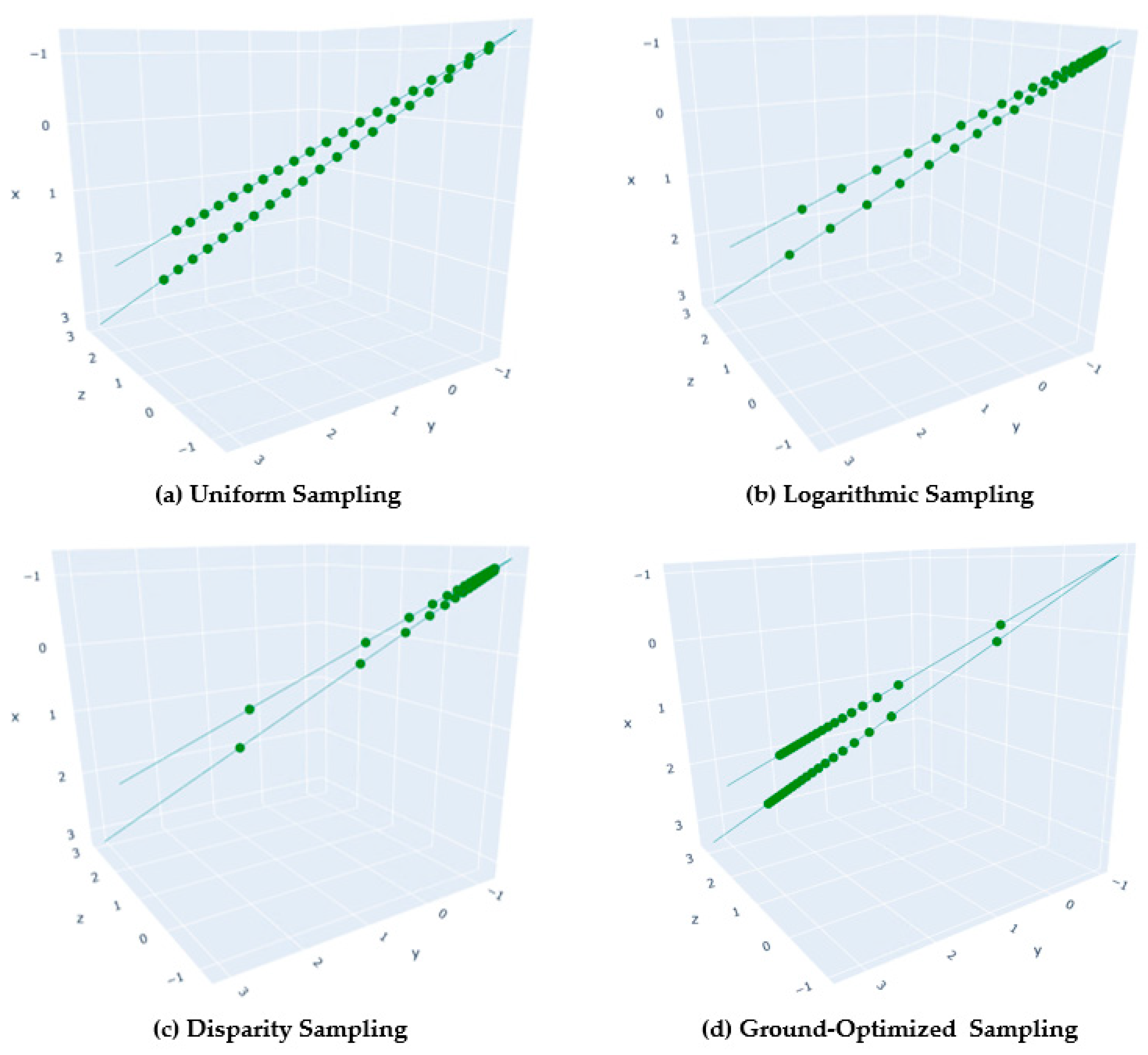
During the rendering of scenes by NeRFs, the process commences by generating a set of rays for each pixel within the image. Subsequently, the algorithm samples points along these rays and queries the neural network to calculate the radiance and volume density for each point. A pivotal challenge lies in determining the positions of these sample points on the rays. The vanilla NeRF [6] employs a Uniform Sampling method, where sample points are allocated equally between the near and far planes, resulting in an excessive allocation of sample points in blank scenes. DoNeRF [13] introduces a Logarithmic Sampling approach, which concentrates more samples closer to the camera, while Mip-NeRF 360 [12] adopts an even more pronounced Disparity Sampling technique, which significantly reduces the sampling distance for close samples, as demonstrated in Figure 3a–c. However, these sampling strategies are not suitable for drone-based scenarios. Drone imagery is often captured from high altitudes, with the camera focusing more on the ground-level scene information rather than areas close to the camera. Adhering to Logarithmic or Disparity Sampling would lead to under-sampling of the ground, which lies farther from the camera, and over-sampling of the air, resulting in an abundance of fluffy artifacts floating above the scene. Dense sampling in areas rich with scene content is crucial; otherwise, the visual quality will be severely compromised.
Therefore, we propose a novel sampling scheme named “Ground-Optimized Sampling”, designed to optimize the distribution of sample points and reduce the frequency of network queries, thereby enhancing the efficiency of the rendering process, as depicted in Figure 3d. The formula for Ground-Optimized Sampling is as follows:
where denotes the origin of the ray, represents the direction of the ray, is the number of the samples placed, and and correspond to the distance from the camera to the near and far planes, respectively. During the execution of Ground-Optimized Sampling, each sample undergoes what is termed “random perturbation”. The unique characteristic of this perturbation is that it maintains the consistency of sample ordering while not altering the overall statistical distribution of the sample group. In addition, we employ a proposal network [12] aimed at further reducing the number of sampling points during training and more effectively concentrating these points on the ground surface. In conclusion, this sampling method concentrates a greater number of sampling points in the areas of the drone-captured scene that are rich in detail, ensuring that even the surfaces at the furthest extents of the scene receive adequate sampling density. This significantly enhances the reconstruction quality of these regions.
4.4. Cluster Sampling
Given that conventional MLP networks primarily tend to learn low-frequency functions [38], they exhibit relatively weaker performance when tasked with fitting high-frequency functions. A solution to this issue is the application of Fourier Encoding, which projects sample points onto the frequency space, causing mutations in Euclidean space to appear relatively smooth in frequency space. This transformation enables the MLP to more easily fit these high-frequency variations, thereby enhancing the resolution of neural rendering results [39]. Similarly, Hash Encoding [18] projects sample points from Euclidean space into hash tables of varying resolutions, allowing grids of different resolutions to capture information at corresponding frequencies. However, both of these encoding methods adopt a discrete form, leading to a single sampling point’s limited ability to capture and represent pixel details at different scales, which results in aliasing effects in distant views. In drone scenarios, the training set naturally leans towards distant views due to the camera’s elevation above the ground.
Mip-NeRF [19] introduced an anti-aliasing encoding strategy. Rather than sampling rays directly for each pixel, it projects a cone and subdivides it into several frustums, which correspond to the sampling intervals. To approximate these frustums, Mip-NeRF employs multivariate Gaussian functions, parameterizing each frustum as a Gaussian distribution with a mean and covariance, thus fitting a uniform distribution of all sampling points within the frustum. Subsequently, this method applies Fourier Encoding to the Gaussian distribution and integrates it, achieving Integrated Fourier Encoding. This strategy effectively prevents the generation of aliasing artifacts in distant views.
To improve the accuracy of scene rendering, increasing the sampling rate is an effective strategy. Inspired by the super-sampling methods in NeRF-SR [40] and LIRF [37], we introduce a novel super-sampling method termed “Cluster Sampling”. This method aims to integrate the advantages of multi-resolution hash grids in terms of speed and memory optimization with the superior distant view rendering capabilities of Integrated Fourier Encoding. In Cluster Sampling, each sampling point on a ray generates a group of additional sampling points, forming a “star cluster”. For each pixel, we cast a cone in the multi-resolution hash grid and use star clusters to approximate each cone section. To fit a uniform distribution of sampling points within a frustum, we sample one point at equal distances in six orthogonal directions around the center point of each frustum. The distance is defined as the radius of a sphere that is tangential to the frustum’s sides and centered on the frustum’s center point. The following formula calculates the new sampling points’ positions:
where represents the coordinates of the original sampling point, is the direction of the ray, denotes the offset vector indicating offsets along the six orthogonal directions of the three-dimensional Cartesian coordinate system, is the radius of the sphere tangential to the frustum sides, is the origin of the ray, is the radius of the frustum’s top surface, and is the distance from the ray’s origin to the top surface of the frustum. is the number of original sampling points.
In Mip-NeRF [19], the scale characteristics of Integrated Fourier Encoding are determined by the covariance of a Gaussian distribution. As shown in Figure 4a, as the covariance increases, the high-frequency encoding gradually decreases to near zero, homogenizing the high-frequency characteristics of all sample points within the frustum. Conversely, as the covariance decreases, the volume of the frustum tends towards a single sampling point, and the Integrated Fourier Encoding will degenerate to the Fourier Encoding of the vanilla NeRF model, thus retaining more high-frequency information. In effect, Integrated Fourier Encoding can be seen as an anti-aliasing Fourier Encoding that allows for the smooth adjustment of encoding space volume and shape. It essentially acts as a Gaussian low-pass filter that can filter out high-frequency signals when rendering low-resolution distant views, achieving an anti-aliasing effect.
Considering that the size of the frustum is proportional to the depth of its location, the decay of the encoding features also increases accordingly. To address this issue, it is necessary to apply a weight to the encoding features of the sample points that decreases with the extension of the ray. By applying Hash Encoding to the star cluster sample points and performing a weighted average, the expected characteristics of the frustum can be determined, thus achieving feature representation of the frustum. This process is called “Integrated Hash Encoding”. Integrated Hash Encoding is designed to achieve a function similar to Integrated Fourier Encoding, as illustrated in Figure 4b. We set a covariance value proportional to the weights of the weighted average Hash Encoding. With an increase in covariance, higher-level grid encoding features will be smoothed to near zero, reducing fluctuations in the high-frequency range. However, as covariance decreases, integrated hash encoding will degenerate to the vanilla Hash Encoding, leading to the reappearance of high-frequency noise. Overall, this encoding method applies diminishing weights to voxel features, thereby balancing the capability to capture details at varying depths. It effectively suppresses the high-frequency noise generated within the hash grid due to excessive discretization, resulting in a more continuous frequency representation post-Hash Encoding.
4.5. Loss Function
In scenarios captured by drones, each image can only capture a limited amount of scene details. Especially for the vanilla NeRF model that utilizes the minimization of mean squared error (MSE) loss, this characteristic could lead to certain issues. Since the model solely relies on the true pixel colors as supervision information when optimizing the radiance field, it might result in overfitting in areas with sparse scene information or encountering local minima during gradient descent, which could produce outliers or noise in those areas. To address this problem, we introduce the L1 norm as a regularization term.
The L1 norm loss, also known as Least Absolute Deviations, can be calculated with the following formula:
where is the predicted value of the pixel, and is the true value of the pixel. The advantage of the L1 loss function is its robustness to outliers, as the penalty it imposes on errors is linear and directly proportional to the size of the error, thus avoiding excessive punishment for larger errors. In contrast, the MSE loss function squares the errors, which can lead to a further magnification of larger errors. Therefore, the L1 loss function is more advantageous in handling outliers.
When the scene includes various transient factors, such as moving objects, changes in lighting, and shadows, which do not persist, there often arise view-dependent effects, or what are called ‘floaters’. This is because the volumetric density prediction in large scenes is not very accurate. To effectively handle these unstable factors, we employ entropy regularization techniques, which tend to encourage opaque rendering and penalize semi-transparent rendering.
Entropy regularization loss is a method that utilizes the concept of information entropy and is inclined to encourage the model to generate outputs with strong certainty (i.e., opacity). In this context, low information entropy means that the distribution of the volumetric density is more likely to be unimodal. Its calculation formula is as follows:
where is the cumulative transmittance, indicating the probability that light travels from the near plane to the far plane without being intercepted, and is the transparency of sample point . This formula is a special form of binary cross-entropy for the case when the true class is 1 (the loss when the true category is 1), and it takes smaller values when is close to 1, thus encouraging the model to generate transparency values close to 1. The goal of entropy regularization loss is to concentrate the weights on the ray into as small a region as possible, thereby optimizing the volumetric density distribution in space.
We chose the following formula to minimize the loss function:
where and are hyperparameters used to balance the main loss items , , and .
5. Results
5.1. Dataset
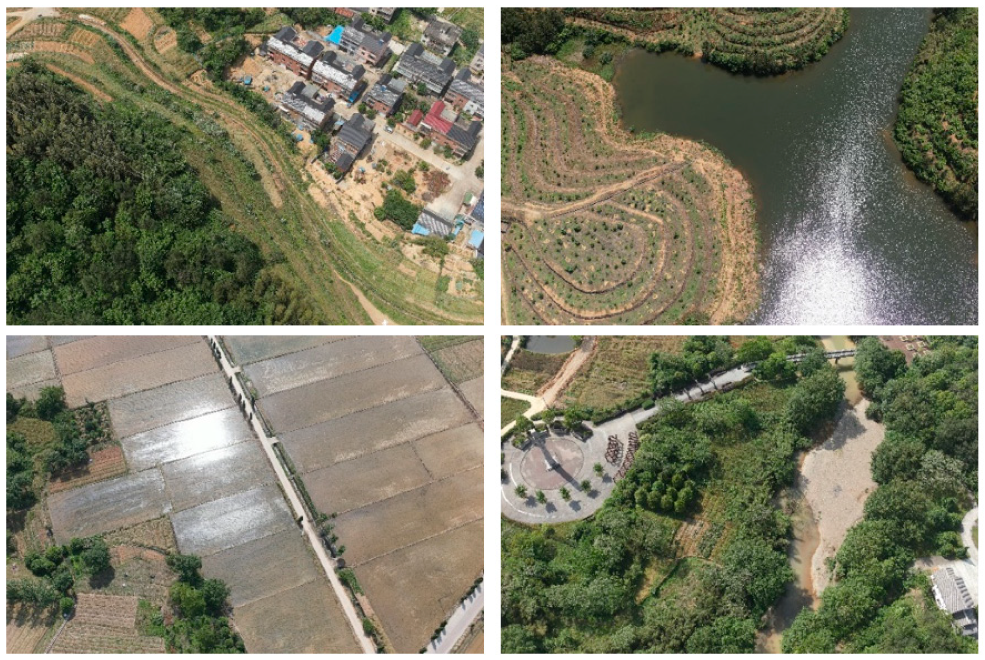
To validate the effectiveness of the proposed framework, we employ circumnavigational flight paths for drone route planning and image capture, using the Metashape 1.8.0 software to restore the camera’s position and orientation. Figure 5 illustrates four distinct scenes in our experiments, each spanning an approximate area of 100,000 square meters. The rural household scene includes a complete village where the rooftops of farmhouses exhibit high reflectivity due to sunlight exposure. The farmland scene encompasses extensive agricultural land, parts of which also show high reflectance due to intense solar radiation. The water body scene comprises a large expanse of water surface, presenting a challenge with its low texture and prominent reflective properties. The vegetation scene covers a vast natural vegetative area, containing many smaller objects. The characteristics of these scenes pose significant challenges in accurately capturing and reproducing the nuanced details of the physical environment. Our method is particularly suited to these static scenes, especially for sampling points near the ground surface, which makes it unsuitable for high-density urban environments. In urban settings, the presence of tall buildings and dynamic factors such as vehicles and pedestrians can interfere with image capture, compromising the effectiveness of the method. Therefore, we chose to focus on natural scenes that are compatible with our methodology, ensuring the accuracy and reliability of our experimental results.
For the dataset, each image with a resolution of 8192 × 5460 was downsampled by a factor of 8. This downsampling is crucial for several reasons. (1) Insufficient Pose Accuracy: High-resolution images make pixel-level pose accuracy difficult, as minor movements cause large pixel shifts. Downsampling reduces this complexity, allowing models to focus on broader, more significant visual features. (2) Incomplete Pixel Coverage: Handling over 44 million pixels per image is not feasible due to hardware and time constraints. Downsampling reduces the number of pixels, enabling more efficient training and better use of computational resources. These adjustments are necessary to balance detail retention with practical computational demands in drone imagery analysis. Of these, 90% of the images were used for model training, while the remaining images were assessed using three image quality metrics, PSNR, SSIM, and LPIPS [41,42,43], to evaluate the model.
5.2. Implementation Details
In the experiments conducted for the framework proposed in this study, the RAdam optimizer was utilized for optimization, with an initial learning rate set at 0.01 and an epsilon value of 1 × 10⁻¹⁵. Throughout the training process, logarithmic decay was applied to adjust the learning rate, gradually reducing it from 0.01 to 0.001. In the allocation of sample points, the experiment incorporated a two-stage proposal network sampling [12], selecting 16 samples in each phase. Subsequently, during the final sampling stage, 8 samples were chosen for optimization. Concerning the configuration of grid parameters, the hierarchy levels of the multi-resolution hash grid were set at 20, with the lowest and highest resolutions established at 16 and 8192, respectively. The hash table was sized at 221, and each entry in the hash table was designed to have a feature dimension of 4. Regarding the model architecture, the MLP used for learning the volumetric density features comprised a layer with 64 neurons, while the MLP for learning appearance features consisted of three layers, each with 256 neurons.
We implemented our proposed method in Nerfstudio [27], a widely used codebase. The framework proposed in this study was implemented on the Windows Server 2022 Standard platform using PyTorch 1.13.1 and CUDA117 and was trained over 30,000 iterations on a Quadro P5000 GPU with 16 GB of VRAM. The batch size for the rays was set at 4096.
5.3. Evaluation
We compare the proposed method against existing methods to demonstrate its effectiveness. The methods for comparison include Mip-NeRF [19], which replaces the ray sampling method used in the vanilla NeRF [6] with an anti-aliasing view-cone sampling method. Instant-NGP [18] introduces a multi-resolution hash grid with learnable parameters. Nerfacto [27] combines the Hash Encoding of Instant-NGP with the Inverse-Sphere Warping of Mip-NeRF 360 [12] to express unbounded scenes. TensoRF [17] employs tensor decomposition algorithms to reduce the memory footprint of the feature grid. Mega-NeRF [14] is a NeRF model designed for drones that uses distributed training to divide large scenes into sub-scenes, each with its own small NeRF model. All NeRF methods, except Mega-NeRF, were trained using the experimental setup, ray batch size, and iteration count described in the previous section.
Specifically, to expand scene representation while avoiding memory overflow, we set the hierarchy levels of the multi-resolution hash grid in Instant NGP to 16, with a maximum resolution of 8192. TensoRF’s highest resolution is set to 512, with 32/96 components used for density and appearance feature grids, respectively. In our study, Mega-NeRF is divided into four sub-blocks. Due to the VRAM constraints of a single GPU, each block is configured with a ray batch size of 2048 and an iteration count of 60,000.
Table 1 presents a comprehensive quantitative comparative analysis between the method proposed in this study and existing NeRF methods. The method we presented outperforms all other listed methods across all evaluation metrics, attaining the highest PSNR and SSIM scores, as well as the lowest LPIPS score, which indicates its closeness to the real image in terms of visual quality. Changes in the PSNR, SSIM, and LPIPS indicators over time during model training are shown in Appendix A. Moreover, the method demonstrates excellence in training time efficiency, requiring only 1.81 h, while Mega-NeRF requires over a week to complete the same task. This drastic reduction in training time is achieved through innovative approaches to sampling and neural network design. Specifically, by optimizing the number of sampling points and employing a streamlined MLP architecture, the proposed method not only expedites the training process but also maintains high-quality rendering outputs, essential for detailed drone scenario visualizations. This suggests that the method achieves a favorable balance between efficiency and quality.
Figure 6 shows the qualitative comparison results between the method of this study and existing NeRF methods. Despite undergoing 30,000 iterations of training, Mip-NeRF failed to converge successfully. Instant-NGP uses multi-level hash grids to represent scenes, significantly shortening training time. However, speckle noise is present across all scenes, and there is a lack of “highlights” information on reflective surface features. Although TensoRF successfully captured some specular reflection information, it performs poorly in presenting distant details. Nerfacto converges quickly in all scenarios but suffers from severe fogging issues in farmland and vegetation scenes. Mega-NeRF exhibits noticeable distortion in high-frequency details, presenting a pronounced blurring effect across all scenes.
In contrast, the method we propose offers significant advantages in the precise replication of real-world scenes in terms of geometric detail and texture sharpness, particularly in the reproduction of roof and photovoltaic details in farmhouse scenarios. In rendering water body scenes, our approach excels in simulating the gloss and reflective effects of water surfaces, presenting a highly realistic visual representation of water and maintaining high accuracy when rendering the vegetation at the water’s edge and the shoreline. For farmland scenes, the proposed method not only accurately presents information on highlights but also captures the fine textural details of vegetation. In scenes with vegetation, our approach demonstrates superior performance in simulating the layering and depth of plant life, with a reproduction of density and color that closely matches the actual landscape. In conclusion, the method we proposed shows significant accuracy in processing scenes captured by drones, particularly excelling in reconstructing the reflection phenomena on object surfaces, and rendering far-distance details that are closer to reality.
5.4. Ablation
We conducted extensive ablation experiments on each component of the proposed framework. All models were trained using the same experimental environment, ray batch size, and iteration count as described in the previous section. The average results of the ablation study are presented in Table 2. Model (A), which combined Inverse-Sphere Warping with Uniform Sampling, produced relatively high LPIPS values, indicating a loss in resolution and texture detail. Models (B) and (C) combined Inverse-Sphere Warping with Logarithmic and Disparity Sampling, respectively, while Model (D) implemented Inverse-Sphere Warping with Ground-Optimized Sampling. Model (E) used Space Boundary Compression with Uniform Sampling, and Models (F) and (G), respectively, combined Space Boundary Compression with Logarithmic and Disparity Sampling. These models exhibited lower metrics when reconstructing drone scenes, reflecting their limitations in effectively restoring scenes. Model (H) disabled Cluster Sampling, resulting in reduced accuracy. Model (I) disabled the L1 loss function, which led to decreased performance. Model (J), when employing Huber loss in place of the combined use of MSE loss and L1 loss, experienced a significant degradation in performance. Model (K) disabled entropy regularization loss, which did not significantly affect the single-image metrics but slightly impaired performance.
In contrast, the proposed method stands out by achieving the highest PSNR of 26.15, the highest SSIM of 0.705, and the lowest LPIPS of 0.298, clearly surpassing all other comparative methods in visual quality. These results thoroughly demonstrate the superiority of the research framework in the field of drone scene reconstruction.
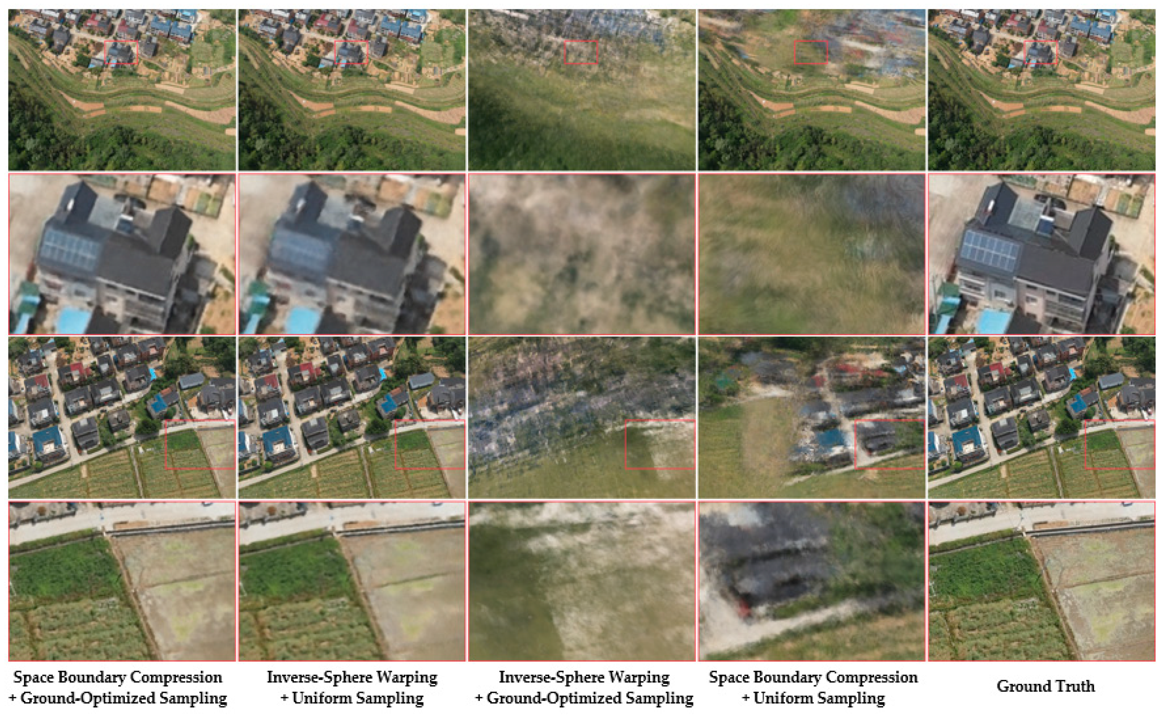
We compared the performance differences between various spatial compression methods and sampling strategies in image rendering through experimental research. Specifically, we analyzed the Inverse-Sphere Warping introduced by Mip-NeRF 360 [12] and the Space Boundary Compression technique proposed in this study. Regarding sampling strategies, in addition to the Uniform Sampling used by the vanilla NeRF model [6], we also examined the Logarithmic Sampling suggested by DoNeRF [13], the Disparity Sampling introduced by Mip-NeRF 360 [12], and a novel Ground-Optimized Sampling method proposed herein.
Figure 7 presents a comparative result of the view quality combining different spatial compression methods with various sampling strategies. It is important to note that even after 30,000 iterations of training, models utilizing Logarithmic and Disparity Sampling strategies failed to adapt to the scene, resulting in a uniformly gray rendering outcome; hence, these results were not displayed in the figure. The combination of Space Boundary Compression with Ground-Optimized Sampling generated images with accurate color restoration, clear edges, and rich texture details. In contrast, the combination of Inverse-Sphere Warping with Uniform Sampling resulted in more pronounced spatial detail distortion, especially in the representation of high-frequency details, such as building contours and field textures. For grasslands sparsely covered with vegetation, this led to an inaccurate distribution of vegetation and caused the photovoltaic panels on the roofs of farmhouses to appear blurred. Images resulting from the combination of Inverse-Sphere Warping with Ground-Optimized Sampling showed a significant decrease in clarity and color fidelity, appearing extremely blurred and nearly devoid of all detail. The images produced by combining Space Boundary Compression with Uniform Sampling exhibited poor global consistency, particularly in the deeper parts of the scene where a noticeable blur effect occurred, accompanied by the incorrect generation of terrain features. In comparison to the real images, it is evident that the method combining Space Boundary Compression with Ground-Optimized Sampling proposed in this paper achieved the highest fidelity in scene reproduction, significantly enhancing the visual clarity and detail representation of landscapes. Meanwhile, other methods underperformed in rendering distant landscape details and lack sufficient accuracy. Overall, experimental results confirm the applicability of Space Boundary Compression to drone-captured surround top-down trajectories, as well as the efficacy of Ground-Optimized Sampling strategies in enhancing the quality of drone scene reconstruction.
As illustrated in Figure 8, the images rendered using the Cluster Sampling technique display more refined and clearer contours of riverbanks, as well as the intricate details of the surrounding vegetation. The reflections and shadows on the water surface are also enhanced, exhibiting more complex textures and well-defined layers. Particularly, for lake surfaces illuminated by sunlight, the application of Cluster Sampling reveals more delicate wave textures and a greater number of ripple effects. By contrast, images produced without Cluster Sampling appear blurrier in terms of edge sharpness and detail resolution. Flat areas on the lake surface show conspicuous speckle noise, and the ripple effects are overly smooth and accompanied by artifacts. The light and shadow effects are also less detailed, resulting in a general deterioration of the image’s texture quality. Comparison with real images demonstrates that Cluster Sampling significantly improves the realism and detail fidelity of rendered images, bringing them closer to the visual experience of actual scenes. This finding confirms the effectiveness of Cluster Sampling in overcoming the limitations of Hash Encoding and enhances the model’s ability to capture scene details, effectively preventing the generation of speckle noise. In summary, Cluster Sampling integrates the advantages of Mip-NeRF and multi-resolution hash grids, thereby augmenting the model’s capacity for detail reproduction and achieving high-precision rendering of distant views.
Figure 9 reveals that, in the absence of an L1 regularization loss during model training, the model incorrectly learned the color of vegetation in farmlands and produced noticeable anomalies on the roads adjacent to the farmlands. For the farmland areas, the rendering outcomes lacking L1 loss exhibited severe blurring and artifacts. In areas where power lines intersect with vegetation, models not utilizing L1 regularization loss did learn the color of the power lines; however, they failed to accurately capture the shape of the power lines, erroneously blending the color of the power lines with the ground vegetation. In contrast, models incorporating L1 regularization loss, along with the model employing Huber loss, were able to effectively ignore the visual interference of power lines on the ground vegetation. The application of L1 regularization loss in scene reconstruction tasks contributes to the production of sharper images and better preservation of high-frequency details. When compared with real images, the ones generated with L1 loss demonstrated superior color accuracy, especially in reproducing details of vegetation and roads. Conversely, images produced without the application of L1 loss displayed fuzzier edges and distorted color representation, performing poorly in detail preservation and noise control. This resulted in a reduction in overall image quality and a significant deviation from the actual scene. Images generated using Huber loss effectively prevent the excessive amplification of larger errors; however, they still lack sufficient capture of high-frequency details, resulting in an overall blurry and unsharp appearance. In conclusion, by incorporating the L1 loss, the model can more effectively restore the detailed structures within images, enhance the generalization capabilities in areas sparse with details, reduce outliers, and maintain structural consistency, thus more authentically mirroring real-world scenes.
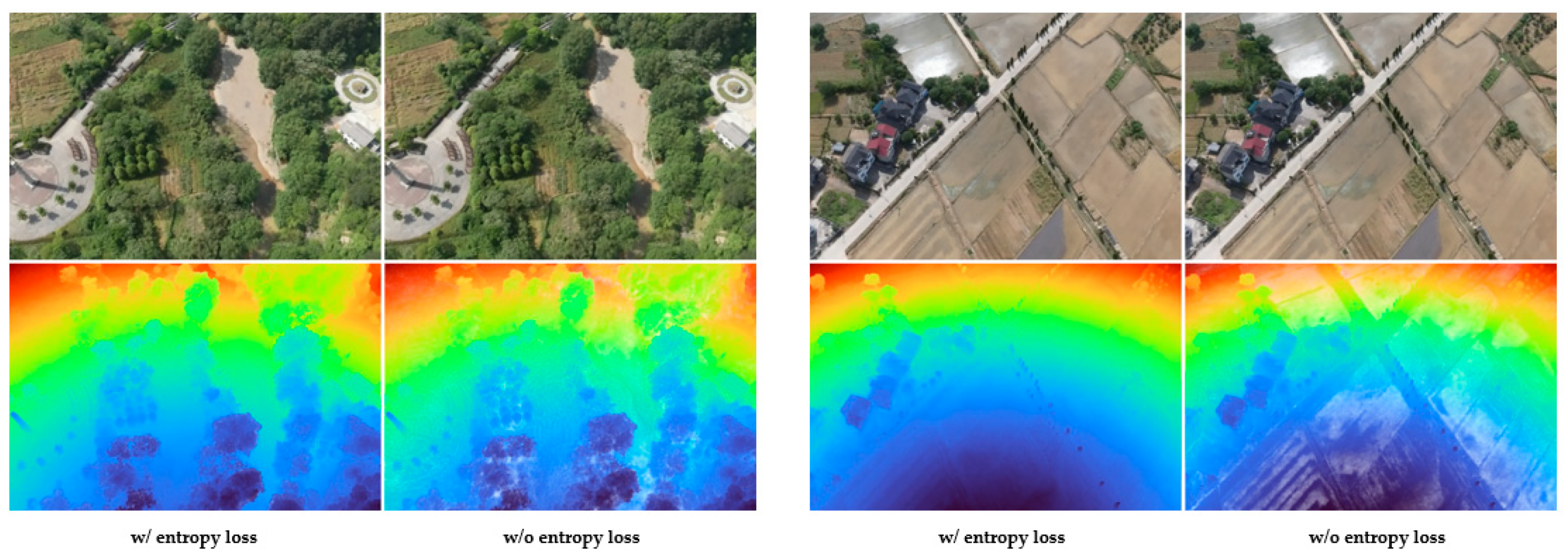
As depicted in Figure 10, the introduction of entropy regularization loss does not markedly impact the visual quality, yet the absence of entropy regularization loss in rendering depth maps reveals specific issues. In regions with dense vegetation, the lack of entropy regularization loss results in the appearance of fluff-like artifacts. In flat farmland areas, a floating phenomenon of semi-transparent objects is observed. Depth maps that employ entropy regularization loss show smoother color transitions, indicating an improvement in the stability and uniformity of depth estimation. In contrast, depth maps without entropy regularization loss exhibit sharp and uneven color variations, revealing increased uncertainty and inconsistency in the model’s spatial prediction. This contrast sharply demonstrates the efficacy of entropy regularization loss in enhancing the quality of depth predictions, particularly when dealing with complex scenes and dynamic factors. Overall, by minimizing information entropy, this loss function aims to concentrate the weights along the ray onto a smaller region, thereby rendering the predictions of volumetric density more focused and precise. This reduction in the uncertainty and inconsistency caused by unstable factors is manifested in depth maps as more concentrated and uniform depth values.
5.5. Limitations
We found that under our current experimental setup, the training of the algorithm is typically confined to a maximum resolution of 1 K. This limitation results in noticeable blurring or distortion when rendering scenes with highly detailed geometric structures. Additionally, although our method can effectively handle data within a certain range, its scalability remains limited under scenarios involving large datasets and high computational demands. These constraints could potentially restrict the practical applicability of our approach, especially in scenarios requiring high-resolution or large-scale data processing.
6. Conclusions and Future Work
We propose a neural rendering framework for drone-captured scenes that caters to the demand for high-quality three-dimensional visualization. The framework utilizes spatial boundary compression technology to divide the 3D space more effectively, which allows for more efficient sampling and significantly reduces the number of network queries. With a ground surface optimization sampling strategy, an abundance of samples is allocated to the content-rich regions of the drone scenes, thus substantially improving the rendering quality of these areas. The integration of Hash Encoding markedly increases the convergence speed of training the NeRF model while avoiding the high video memory consumption associated with querying a vast neural network. By applying a Cluster Sampling technique, the frequency information after Hash Encoding becomes more coherent, achieving rendering accuracy at the sub-pixel level. Moreover, the use of an L1 photometric loss makes the model less sensitive to anomalies, thereby lowering the noise level in image reconstruction and successfully decreasing rendering biases. By minimizing entropy regularization loss, the system penalizes semi-transparent renderings and promotes the production of opaque outputs, effectively suppressing the erroneous generation of fluffy artifacts and semi-transparent materials within the scene, thereby significantly enhancing the scene’s visual quality.
Experimental findings demonstrate that this framework is more apt for drone-captured scenes compared to previous NeRF methods, attaining an optimized effect in 3D scene visualization quality. In terms of rendering outcomes, the framework significantly preserves “highlight” information on reflective ground surfaces, notably reducing speckle noise and rendering inaccuracies, while the representation of distant details closely matches the actual environment. This framework achieves a balance between expediting the training process and improving rendering quality by prioritizing computational resource allocation to the most detail-rich areas of the scene and using a series of optimization strategies to make efficient use of the limited sample budget. We plan to introduce several key technologies in our future research to enhance system performance and scalability. First, to address the resolution limitations, we will explore the use of super-resolution algorithms [44] to enhance the detail rendering capabilities of our images. Furthermore, considering the need for real-time rendering, we plan to employ baking algorithms [26] to accelerate the rendering process. To improve the scalability of our system, we will test our method on larger datasets and consider integrating more advanced computational techniques and specific scaling technologies. Specifically, we will investigate vertical scaling technologies [35,45] designed for generating data representations at varying scales, including earth-scale, which are crucial for efficiently processing extensive scenes; we will also explore horizontal scaling [14] through distributed processing, ensuring our method can handle broader scenes while maintaining quality and coherence. Additionally, to overcome the limitations encountered with a single GPU when processing large-scale and complex datasets, we plan to adopt a multi-GPU system in our future research.
By implementing these plans, we aim to significantly enhance the practical performance and adaptability of our method. Inspired by findings from [46], we also plan to design new metrics that effectively describe the rendering quality of NeRF models across various spatial scales and resolutions, thereby enhancing the efficiency of rendering effect assessments.
Author Contributions
Conceptualization, P.J. and Z.Y.; methodology, P.J.; software, P.J.; validation, P.J.; formal analysis, P.J.; investigation, P.J.; resources, Z.Y.; data curation, P.J.; writing—original draft preparation, P.J.; writing—review and editing, Z.Y.; visualization, P.J.; supervision, Z.Y.; project administration, Z.Y.; funding acquisition, Z.Y. All authors have read and agreed to the published version of the manuscript.
Funding
This research was funded by the National Key R&D Program (grant number: 2022YFF0711605).
Data Availability Statement
The data are not publicly available due to privacy and can be obtained upon reasonable request.
Conflicts of Interest
The authors declare no conflicts of interest.
Appendix A
This appendix includes graphs depicting the changes in Peak Signal-to-Noise Ratio (PSNR), Structural Similarity Index Measure (SSIM), and Learned Perceptual Image Patch Similarity (LPIPS) over time for each tested scenario. As depicted in Figure A1, these graphs quantitatively demonstrate how the performance metrics of our model evolve as a function of training time. In the graphs, the horizontal axis represents time, showing the progression of model optimization over the duration of the training. The vertical axis represents the metric values, where typically, the graphs for PSNR and SSIM exhibit an upward trend, indicating improvements in image fidelity and structural similarity as training progresses. Conversely, the graphs for LPIPS generally show a downward trend, reflecting enhanced perceptual similarity between the generated images and the ground truth. These visualizations help to understand the convergence behavior of our model and highlight the effectiveness of the training methodology used in this study.
Figure A1.
Temporal Evolution of PSNR, SSIM, and LPIPS Metrics During Model Training.

References
- Lombardi, S.; Simon, T.; Saragih, J.; Schwartz, G.; Lehrmann, A.; Sheikh, Y. Neural volumes: Learning dynamic renderable volumes from images. arXiv 2019, arXiv:1906.07751. [Google Scholar] [CrossRef]
- Mescheder, L.; Oechsle, M.; Niemeyer, M.; Nowozin, S.; Geiger, A. Occupancy networks: Learning 3d reconstruction in function space. In Proceedings of the IEEE/CVF Conference on Computer Vision and Pattern Recognition, Long Beach, CA, USA, 15–20 June 2019; pp. 4460–4470. [Google Scholar] [CrossRef]
- Park, J.J.; Florence, P.; Straub, J.; Newcombe, R.; Lovegrove, S. Deepsdf: Learning continuous signed distance functions for shape representation. In Proceedings of the IEEE/CVF Conference on Computer Vision and Pattern Recognition, Long Beach, CA, USA, 15–20 June 2019; pp. 165–174. [Google Scholar] [CrossRef]
- Niemeyer, M.; Mescheder, L.; Oechsle, M.; Geiger, A. Differentiable volumetric rendering: Learning implicit 3d representations without 3d supervision. In Proceedings of the IEEE/CVF Conference on Computer Vision and Pattern Recognition, Long Beach, CA, USA, 15–20 June 2019; pp. 3504–3515. [Google Scholar] [CrossRef]
- Schirmer, L.; Schardong, G.; da Silva, V.; Lopes, H.; Novello, T.; Yukimura, D.; Magalhaes, T.; Paz, H.; Velho, L. Neural networks for implicit representations of 3D scenes. In Proceedings of the 34th SIBGRAPI Conference on Graphics, Patterns and Images (SIBGRAPI), Gramado, Rio Grande do Sul, Brazil, 18–22 October 2021; pp. 17–24. [Google Scholar] [CrossRef]
- Mildenhall, B.; Srinivasan, P.P.; Tancik, M.; Barron, J.T.; Ramamoorthi, R.; Ng, R. Nerf: Representing scenes as neural radiance fields for view synthesis. Commun. ACM 2021, 65, 99–106. [Google Scholar] [CrossRef]
- Li, K.; Rolff, T.; Schmidt, S.; Bacher, R.; Frintrop, S.; Leemans, W.; Steinicke, F. Bringing instant neural graphics primitives to immersive virtual reality. In Proceedings of the IEEE Conference on Virtual Reality and 3D User Interfaces Abstracts and Workshops (VRW), Shanghai, China, 25–29 March 2023; pp. 739–740. [Google Scholar] [CrossRef]
- Wu, Z.; Liu, T.; Luo, L.; Zhong, Z.; Chen, J.; Xiao, H.; Hou, C.; Lou, H.; Chen, Y.; Yang, R.; et al. Mars: An instance-aware, modular and realistic simulator for autonomous driving. In Proceedings of the CAAI International Conference on Artificial Intelligence, Fuzhou, China, 22–23 July 2023; Springer Nature: Singapore, 2023; pp. 3–15. [Google Scholar]
- Kerr, J.; Fu, L.; Huang, H.; Avigal, Y.; Tancik, M.; Ichnowski, J.; Kanazawa, A.; Goldberg, K. Evo-nerf: Evolving nerf for sequential robot grasping of transparent objects. In Proceedings of the 6th Annual Conference on Robot Learning, Auckland, New Zealand, 14–18 December 2022. [Google Scholar]
- Tancik, M.; Casser, V.; Yan, X.; Pradhan, S.; Mildenhall, B.; Srinivasan, P.P.; Barron, J.T.; Kretzschmar, H. Block-nerf: Scalable large scene neural view synthesis. In Proceedings of the IEEE/CVF Conference on Computer Vision and Pattern Recognition, New Orleans, LA, USA, 18–24 June 2022; pp. 8248–8258. [Google Scholar] [CrossRef]
- Luma Labs. Available online: https://lumalabs.ai/ (accessed on 2 April 2024).
- Barron, J.T.; Mildenhall, B.; Verbin, D.; Srinivasan, P.P.; Hedman, P. Mip-nerf 360: Unbounded anti-aliased neural radiance fields. In Proceedings of the IEEE/CVF Conference on Computer Vision and Pattern Recognition, New Orleans, LA, USA, 18–24 June 2022; pp. 5470–5479. [Google Scholar] [CrossRef]
- Neff, T.; Stadlbauer, P.; Parger, M.; Kurz, A.; Mueller, J.H.; Chaitanya, C.R.A.; Kaplanyan, A.; Steinberger, M. DONeRF: Towards Real-Time Rendering of Compact Neural Radiance Fields using Depth Oracle Networks. Comput. Graph. Forum 2021, 40, 45–59. [Google Scholar] [CrossRef]
- Turki, H.; Ramanan, D.; Satyanarayanan, M. Mega-nerf: Scalable construction of large-scale nerfs for virtual fly-throughs. In Proceedings of the IEEE/CVF Conference on Computer Vision and Pattern Recognition, New Orleans, LA, USA, 18–24 June 2022; pp. 12922–12931. [Google Scholar] [CrossRef]
- Sun, C.; Sun, M.; Chen, H.T. Direct voxel grid optimization: Super-fast convergence for radiance fields reconstruction. In Proceedings of the IEEE/CVF Conference on Computer Vision and Pattern Recognition, New Orleans, LA, USA, 18–24 June 2022; pp. 5459–5469. [Google Scholar] [CrossRef]
- Fridovich-Keil, S.; Yu, A.; Tancik, M.; Chen, Q.; Recht, B.; Kanazawa, A. Plenoxels: Radiance fields without neural networks. In Proceedings of the IEEE/CVF Conference on Computer Vision and Pattern Recognition, New Orleans, LA, USA, 18–24 June 2022; pp. 5501–5510. [Google Scholar] [CrossRef]
- Chen, A.; Xu, Z.; Geiger, A.; Yu, J.; Su, H. TensorF: Tensorial Radiance Fields. In Proceedings of the European Conference on Computer Vision, Tel Aviv, Israel, 23–27 October 2022; Springer Nature: Cham, Switzerland, 2022; pp. 333–350. [Google Scholar] [CrossRef]
- Müller, T.; Evans, A.; Schied, C.; Keller, A. Instant neural graphics primitives with a multiresolution hash encoding. ACM Trans. Graph. (TOG) 2022, 41, 1–15. [Google Scholar] [CrossRef]
- Barron, J.T.; Mildenhall, B.; Tancik, M.; Hedman, P.; Martin-Brualla, R.; Srinivasan, P.P. Mip-nerf: A multiscale representation for anti-aliasing neural radiance fields. In Proceedings of the IEEE/CVF International Conference on Computer Vision, Montreal, BC, Canada, 11–17 October 2021; pp. 5855–5864. [Google Scholar] [CrossRef]
- Arandjelović, R.; Zisserman, A. Nerf in detail: Learning to sample for view synthesis. arXiv 2021, arXiv:2106.05264. [Google Scholar]
- Xu, B.; Wu, L.; Hasan, M.; Luan, F.; Georgiev, I.; Xu, Z.; Ramamoorthi, R. NeuSample: Importance Sampling for Neural Materials. In Proceedings of the ACM SIGGRAPH 2023 Conference, Los Angeles, CA, USA, 6–10 August 2023; pp. 1–10. [Google Scholar] [CrossRef]
- Kurz, A.; Neff, T.; Lv, Z.; Zollhöfer, M.; Steinberger, M. Adanerf: Adaptive sampling for real-time rendering of neural radiance fields. In Proceedings of the European Conference on Computer Vision, Tel Aviv, Israel, 23–27 October 2022; Springer Nature: Cham, Switzerland, 2022; pp. 254–270. [Google Scholar] [CrossRef]
- Lin, H.; Peng, S.; Xu, Z.; Yan, Y.; Shuai, Q.; Bao, H.; Zhou, X. Efficient neural radiance fields for interactive free-viewpoint video. In Proceedings of the SIGGRAPH Asia 2022 Conference Papers, Daegu, Republic of Korea, 6–9 December 2022; pp. 1–9. [Google Scholar] [CrossRef]
- Piala, M.; Clark, R. Terminerf: Ray termination prediction for efficient neural rendering. In Proceedings of the 2021 International Conference on 3D Vision (3DV), London, UK, 1–3 December 2021; pp. 1106–1114. [Google Scholar] [CrossRef]
- Zhang, K.; Riegler, G.; Snavely, N.; Koltun, V. Nerf++: Analyzing and improving neural radiance fields. arXiv 2020, arXiv:2010.07492. [Google Scholar]
- Reiser, C.; Szeliski, R.; Verbin, D.; Srinivasan, P.; Mildenhall, B.; Geiger, A.; Barron, J.; Hedman, P. Merf: Memory-Efficient Radiance Fields for Real-Time View Synthesis in Unbounded Scenes. ACM Trans. Graph. 2023, 42, 1–12. [Google Scholar] [CrossRef]
- Tancik, M.; Weber, E.; Ng, E.; Li, R.; Yi, B.; Wang, T.; Kristoffersen, A.; Austin, J.; Salahi, K.; Ahuja, A.; et al. Nerf-Studio: A Modular Framework for Neural Radiance Field Development. In Proceedings of the ACM SIGGRAPH 2023 Conference, Los Angeles, CA, USA, 6–10 August 2023; pp. 1–12. [Google Scholar] [CrossRef]
- Yu, X.; Wang, H.; Han, Y.; Yang, L.; Yu, T.; Dai, Q. ImmersiveNeRF: Hybrid Radiance Fields for Unbounded Immersive Light Field Reconstruction. arXiv 2023, arXiv:2309.01374. [Google Scholar]
- He, Y.; Wang, P.; Hu, Y.; Zhao, W.; Yi, R.; Liu, Y.J.; Wang, W. MMPI: A Flexible Radiance Field Representation by Multiple Multi-plane Images Blending. arXiv 2023, arXiv:2310.00249. [Google Scholar]
- Phongthawee, P.; Wizadwongsa, S.; Yenphraphai, J.; Suwajanakorn, S. Nex360: Real-Time All-Around View Synthesis with Neural Basis Expansion. IEEE Trans. Pattern Anal. Mach. Intell. 2022, 45, 7611–7624. [Google Scholar] [CrossRef]
- Mi, Z.; Xu, D. Switch-NeRF: Learning Scene Decomposition with Mixture of Experts for Large-Scale Neural Radiance Fields. In Proceedings of the Eleventh International Conference on Learning Representations, Kigali, Rwanda, 1–5 May 2023. [Google Scholar]
- Rematas, K.; Liu, A.; Srinivasan, P.P.; Barron, J.T.; Tagliasacchi, A.; Funkhouser, T.; Ferrari, V. Urban Radiance Fields. In Proceedings of the IEEE/CVF Conference on Computer Vision and Pattern Recognition, New Orleans, LA, USA, 18–24 June 2022; pp. 12932–12942. [Google Scholar] [CrossRef]
- Turki, H.; Zhang, J.Y.; Ferroni, F.; Ramanan, D. Suds: Scalable Urban Dynamic Scenes. In Proceedings of the IEEE/CVF Conference on Computer Vision and Pattern Recognition, Vancouver, BC, Canada, 17–24 June 2023; pp. 12375–12385. [Google Scholar] [CrossRef]
- Liu, L.; Gu, J.; Lin, K.Z.; Chua, T.S.; Theobalt, C. Neural Sparse Voxel Fields. Adv. Neural Inf. Process. Syst. 2020, 33, 15651–15663. [Google Scholar]
- Xiangli, Y.; Xu, L.; Pan, X.; Zhao, N.; Rao, A.; Theobalt, C.; Dai, B.; Lin, D. BungeeNeRF: Progressive Neural Radiance Field for Extreme Multi-Scale Scene Rendering. In Proceedings of the European Conference on Computer Vision, Tel Aviv, Israel, 23–27 October 2022; Springer Nature: Cham, Switzerland, 2022; pp. 106–122. [Google Scholar] [CrossRef]
- Isaac-Medina, B.K.; Willcocks, C.G.; Breckon, T.P. Exact-NeRF: An Exploration of a Precise Volumetric Parameterization for Neural Radiance Fields. In Proceedings of the IEEE/CVF Conference on Computer Vision and Pattern Recognition, Vancouver, BC, Canada, 17–24 June 2023; pp. 66–75. [Google Scholar] [CrossRef]
- Huang, X.; Zhang, Q.; Feng, Y.; Li, X.; Wang, X.; Wang, Q. Local Implicit Ray Function for Generalizable Radiance Field Representation. In Proceedings of the IEEE/CVF Conference on Computer Vision and Pattern Recognition, Vancouver, BC, Canada, 17–24 June 2023; pp. 97–107. [Google Scholar] [CrossRef]
- Rahaman, N.; Baratin, A.; Arpit, D.; Draxler, F.; Lin, M.; Hamprecht, F.; Bengio, Y.; Courville, A. On the Spectral Bias of Neural Networks. In Proceedings of the International Conference on Machine Learning, Long Beach, CA, USA, 9–15 June 2019; pp. 5301–5310. [Google Scholar]
- Tancik, M.; Srinivasan, P.; Mildenhall, B.; Fridovich-Keil, S.; Raghavan, N.; Singhal, U.; Ramamoorthi, R.; Barron, J.; Ng, R. Fourier Features Let Networks Learn High Frequency Functions in Low Dimensional Domains. Adv. Neural Inf. Process. Syst. 2020, 33, 7537–7547. [Google Scholar]
- Wang, C.; Wu, X.; Guo, Y.C.; Zhang, S.H.; Tai, Y.W.; Hu, S.M. NeRF-SR: High Quality Neural Radiance Fields Using Supersampling. In Proceedings of the 30th ACM International Conference on Multimedia, Lisboa, Portugal, 10–14 October 2022; pp. 6445–6454. [Google Scholar] [CrossRef]
- Korhonen, J.; You, J. Peak Signal-to-Noise Ratio Revisited: Is Simple Beautiful? In Proceedings of the 2012 Fourth International Workshop on Quality of Multimedia Experience, Melbourne, VIC, Australia, 5–7 July 2012; pp. 37–38. [Google Scholar]
- Wang, Z.; Bovik, A.C.; Sheikh, H.R.; Simoncelli, E.P. Image Quality Assessment: From Error Visibility to Structural Similarity. IEEE Trans. Image Process. 2004, 13, 600–612. [Google Scholar] [CrossRef]
- Zhang, R.; Isola, P.; Efros, A.A.; Shechtman, E.; Wang, O. The Unreasonable Effectiveness of Deep Features as a Perceptual Metric. In Proceedings of the IEEE Conference on Computer Vision and Pattern Recognition, Salt Lake City, UT, USA, 18–23 June 2018; pp. 586–595. [Google Scholar] [CrossRef]
- Wang, Z.; Li, L.; Shen, Z.; Shen, L.; Bo, L. 4K-NeRF: High Fidelity Neural Radiance Fields at Ultra High Resolutions. arXiv 2022, arXiv:2212.04701. [Google Scholar]
- Tabassum, A.; Basak, R.; Shao, W.; Haque, M.M.; Chowdhury, T.A.; Dey, H. Exploring the relationship between land use land cover and land surface temperature: A case study in Bangladesh and the policy implications for the Global South. J. Geovisualization Spat. Anal. 2023, 7, 25. [Google Scholar] [CrossRef]
- Masoudi, M.; Richards, D.R.; Tan, P.Y. Assessment of the Influence of Spatial Scale and Type of Land Cover on Urban Landscape Pattern Analysis Using Landscape Metrics. J. Geovisualization Spat. Anal. 2024, 8, 8. [Google Scholar] [CrossRef]
Figure 1.
Overview: This figure illustrates the complete process from initial sampling to final rendering. The black arrows represent the rays in the sampling scenarios, while the yellow arrows indicate the arrows in the flowchart.
Figure 1.
Overview: This figure illustrates the complete process from initial sampling to final rendering. The black arrows represent the rays in the sampling scenarios, while the yellow arrows indicate the arrows in the flowchart.

Figure 2.
Schematic diagrams of various spatial compression methods and camera trajectory. Top: (a) forward-facing camera trajectory; (b) 360° object-centric camera trajectory; (c) drone-captured surround top–down trajectory, highlighting the complex and sparse nature of drone camera paths. Bottom: (a) NDC Warping; (b) Inverse-Sphere Warping; (c) Space Boundary Compression, which optimizes sampling by eliminating minimally contributing regions.

Figure 3.
Schematic diagram of various sampling methods: (a) Uniform Sampling; (b) Logarithmic Sampling; (c) Disparity Sampling; (d) Ground-Optimized Sampling, increasing sampling points in areas rich in detail.
Figure 3.
Schematic diagram of various sampling methods: (a) Uniform Sampling; (b) Logarithmic Sampling; (c) Disparity Sampling; (d) Ground-Optimized Sampling, increasing sampling points in areas rich in detail.

Figure 4.
Schematic diagram of various encoding methods: (a) vanilla Fourier Encoding and Integrated Fourier Encoding with various covariances; (b) vanilla Hash Encoding and Integrated Hash Encoding with various covariances.
Figure 4.
Schematic diagram of various encoding methods: (a) vanilla Fourier Encoding and Integrated Fourier Encoding with various covariances; (b) vanilla Hash Encoding and Integrated Hash Encoding with various covariances.

Figure 5.
Dataset: our dataset contains 4 scenes. Among these, there are expansive low-texture water surfaces, densely vegetated areas, and farmlands with strong reflections, factors that render the reconstruction task particularly challenging.
Figure 5.
Dataset: our dataset contains 4 scenes. Among these, there are expansive low-texture water surfaces, densely vegetated areas, and farmlands with strong reflections, factors that render the reconstruction task particularly challenging.

Figure 6.
Qualitative comparison results with existing NeRF methods.

Figure 7.
Qualitative comparison results of different space compression methods and sampling strategy combinations.
Figure 7.
Qualitative comparison results of different space compression methods and sampling strategy combinations.

Figure 8.
Qualitative comparison results with and without applying Cluster Sampling.

Figure 9.
Qualitative comparison results with and without L1 loss, and with Huber loss.

Figure 10.
Qualitative comparison results with and without applying entropy loss.


Table 1.
Quantitative comparison results with existing NeRF methods. We report PSNR (↑), SSIM (↑), and LPIPS (↓) metrics on the test view. ↑ means higher value is better, while ↓ means lower value is better. The best results are bolded.
Table 1.
Quantitative comparison results with existing NeRF methods. We report PSNR (↑), SSIM (↑), and LPIPS (↓) metrics on the test view. ↑ means higher value is better, while ↓ means lower value is better. The best results are bolded.
| Methods | PSNR ↑ | SSIM ↑ | LPIPS ↓ | Time (h) |
|---|---|---|---|---|
| Mip-NeRF | 14.39 | 0.418 | 0.845 | 11.50 |
| Instant-NGP | 23.54 | 0.657 | 0.378 | 2.45 |
| Nerfacto | 25.08 | 0.683 | 0.324 | 1.44 |
| TensoRF | 24.65 | 0.622 | 0.394 | 8.57 |
| Mega-NeRF | 22.84 | 0.488 | 0.596 | 178.10 |
| Proposed method | 26.15 | 0.705 | 0.298 | 1.81 |
Table 2.
Quantitative comparison results with ablation experiment. ↑ means higher value is better, while ↓ means lower value is better. The best results are bolded.
Table 2.
Quantitative comparison results with ablation experiment. ↑ means higher value is better, while ↓ means lower value is better. The best results are bolded.
| Methods | PSNR ↑ | SSIM ↑ | LPIPS ↓ |
|---|---|---|---|
| (A) Inverse-Sphere Warping + Uniform Sampling | 25.89 | 0.681 | 0.341 |
| (B) Inverse-Sphere Warping + Logarithmic Sampling | 15.46 | 0.434 | 0.852 |
| (C) Inverse-Sphere Warping + Disparity Sampling | 16.09 | 0.440 | 0.851 |
| (D) Inverse-Sphere Warping + Ground-Optimized Sampling | 17.17 | 0.396 | 0.676 |
| (E) Space Boundary Compression + Uniform Sampling | 15.04 | 0.358 | 0.711 |
| (F) Space Boundary Compression + Logarithmic Sampling | 14.41 | 0.424 | 0.913 |
| (G) Space Boundary Compression + Disparity Sampling | 14.41 | 0.424 | 0.913 |
| (H) w/o Cluster Sampling | 26.00 | 0.693 | 0.311 |
| (I) w/o L1 Loss | 25.98 | 0.693 | 0.305 |
| (J) w Huber Loss | 25.85 | 0.682 | 0.323 |
| (K) w/o Entropy Loss | 26.12 | 0.703 | 0.300 |
| Proposed method | 26.15 | 0.705 | 0.298 |
Disclaimer/Publisher’s Note: The statements, opinions and data contained in all publications are solely those of the individual author(s) and contributor(s) and not of MDPI and/or the editor(s). MDPI and/or the editor(s) disclaim responsibility for any injury to people or property resulting from any ideas, methods, instructions or products referred to in the content. |
© 2024 by the authors. Licensee MDPI, Basel, Switzerland. This article is an open access article distributed under the terms and conditions of the Creative Commons Attribution (CC BY) license (https://creativecommons.org/licenses/by/4.0/).
Share and Cite
MDPI and ACS Style
Jin, P.; Yu, Z. Research on 3D Visualization of Drone Scenes Based on Neural Radiance Fields. Electronics 2024, 13, 1682. https://doi.org/10.3390/electronics13091682
AMA Style
Jin P, Yu Z. Research on 3D Visualization of Drone Scenes Based on Neural Radiance Fields. Electronics. 2024; 13(9):1682. https://doi.org/10.3390/electronics13091682
Chicago/Turabian StyleJin, Pengfei, and Zhuoyuan Yu. 2024. "Research on 3D Visualization of Drone Scenes Based on Neural Radiance Fields" Electronics 13, no. 9: 1682. https://doi.org/10.3390/electronics13091682
Note that from the first issue of 2016, this journal uses article numbers instead of page numbers. See further details here.