Virtual Machine Replication on Achieving Energy-Efficiency in a Cloud

Abstract

The rapid growth in cloud service demand has led to the establishment of large-scale virtualized data centers in which virtual machines (VMs) are used to handle user requests for service. A user’s request cannot be completed if the VM fails. Replication mechanisms can be used to mitigate the impact of failures. Further, data centers consume a large amount of energy resulting in high operating costs and contributing to significant greenhouse gas (GHG) emissions. In this paper, we focus on Infrastructure as a Service (IaaS) cloud where user job requests are processed by VMs and analyze the effectiveness of VM replications in terms of job completion time performance as well as energy consumption. Three different schemes: cold, warm, and hot replications are considered. The trade-offs between job completion time and energy consumption in different replication schemes are characterized through comprehensive analytical models which capture VM state transitions and associated power consumption patterns. The effectiveness of replication schemes are demonstrated through experimental results. To verify the validity of the proposed analytical models, we extend the widely used cloud simulator CloudSim and compare the simulation results with analytical solutions.

1. Introduction

Cloud computing is a realization of the endeavour to provide computing as a utility. Users submit their work requests to the cloud, to be processed and the results are delivered. Typically, the rapid growth in demand for computational power driven by modern service-oriented applications has led to the establishment of large-scale virtualized data centers [1,2,3,4]. However, data centers consume a huge amount of energy resulting in high operating costs and resulting contribution to greenhouse gas (GHG) emissions. A major reason for this significant power consumption is the inefficiency of data center deployments, which are often underutilized. It has been estimated that only 10%–50% of the total server capacity is used on average [3,5].

A job in a system may be interrupted/preempted due to any failures of the system components. The interruption/preemption of job execution not only affects the job completion time performance, but also results in additional energy consumption. In order to alleviate the impacts of job interruption, replication of job execution gives a viable mean [6,7]. Further, data replication and software process redundancy are common practices in cloud computing systems [6,7]. In addition, Bauer et al. [7] presents different types of VM redundancy for enhancing service reliability in cloud. We can ensure service reliability at different satisfactory levels by VM redundancy based on its appliances.

Further, building trustworthy cloud is one of the main challenges faced by the providers. Malicious attacks and software errors are increasingly common. The growing reliance of industry and government on online information services makes malicious attacks more attractive and makes the consequences of successful attacks more serious. In addition, the number of software errors is increasing due to the growth in size and complexity of software. Malicious attacks and software errors can cause faulty nodes to exhibit Byzantine (i.e., arbitrary) behavior [8] in which components of a system fail in arbitrary ways (i.e., not just by stopping or crashing but by processing requests incorrectly, corrupting their local state, and/or producing incorrect or inconsistent outputs). It is mandatory to have Byzantine Fault Tolerant (BFT) mechanism to defend against Byzantine failures so that a system can continue to operate correctly even if some of its components exhibit arbitrary, possibly malicious behavior. We need to use replication techniques to tolerate/sustain/defend Byzantine fault as suggested by Byzantine Generals’ Problem [8]; would have at least $3f+1$ replicas where f be the maximum number of replicas that may be faulty. Further, Hadoop distributed file system (HDFS) uses the default replication value of 3 for enhancing fault tolerance [9]. Thus, replication/redundancy is common practice in cloud. In this paper, we focus on analyzing energy consumption optimization rather than security issues, so we concentrate on different schemes of 1 + 1 replication (one instance works as primary and another instance as standby) and show the effectiveness on energy consumption as well as job completion time. If we use more than one redundant copies, then energy consumption will rise.

In this paper, we provide models for analyzing the job execution process in cloud computing environment under different schemes of 1 + 1 replication. Specifically, our analysis is based on the VM provisioning model for the cloud [1,2], where a VM is deployed on a physical machine (PM) upon arrival of a user request, and each request (job) has work requirement which is represented by the computation time on a failure-free environment. The actual job completion time may become longer than the given work requirement because of occurrences of VM or PM failures and subsequent recovery process with or without replication. We can represent the job execution interruption/preemption due to VM or PM failure and restarting/resuming upon recovery by structure-state process [10,11] that is semi-Markov process (SMP), representing system state transitions. The interruption/preemption interactions of job execution are categorized as $i)$ preemptive-resume (prs)—resumes execution from the point of interruption, $ii)$ preemptive-repeat-identical (pri or prt)—the interrupted job is restarted from the beginning and have the identical work requirement as the original interrupted job, and $iii)$ preemptive-repeat-different (prd)—the interrupted job is restarted with a new work requirement which is statistically independent, and identically distributed to the original work requirement [10,11,12]. The job execution time and associated energy consumption in different replication schemes are investigated in consideration with the above-mentioned preemption types. The experimental results on the proposed model enables us to compare the effectiveness of different replication schemes in terms of both job execution performance and energy efficiency.

The rest of this paper is organized as follows: we discuss the related work in Section 2. In Section 3.1, we describe the system model. The basic concept of cloud service implementation under the replication scheme is addressed in Section 3.2. We present the power consumption model in Section 4.1. A brief discussion on job completion time formulation is presented in Section 4.2. In Section 5, we show the analytic models of job execution and derive closed-form expressions for the computation of job completion time and the measurement of energy consumption in different replication schemes. Experimental results are shown in Section 6. Conclusions and future work are given in the final section.

2. Related Work

Mastroianni et al. [3,5] showed the statistical consolidation of VMs in data centers. They discussed the assignment of new VMs and migration of running VMs by considering upper and lower CPU utilization threshold of PMs so that the system does not become overloaded and does not violate quality of service (QoS).

Buyya et al. [4] discussed energy-aware resource allocation using greedy bin packing problem. They used a modification of the Best Fit Decreasing (BFD) algorithm for new VMs assignment and running VMs migration. They also took into account the upper and lower CPU utilization threshold of PMs for the assignment and migration of VMs.

The approaches proposed by Mastroianni et al. [3,5] and Buyya et al. [4] mainly discuss how we can consolidate jobs among fewer number of servers and put the servers with very low and with very high CPU utilization to sleep mode or turn-off mode. In sleep mode power consumption is very much low [13,14,15].

Cloud systems experience frequent failures due to their large-scale and distributed nature [16]. Failures of any components in the cloud may cause the jobs to be interrupted. Jobs may span thousands of cloud components and run for a long time before being interrupted, which leads to the wastage of energy and other resources [16]. Thus, one of the main challenges in cloud systems is to assure the reliability of job execution in the presence of failures. Specifically, if a job is restarted upon failure, the energy consumed for the segment of the job that has been executed before the failure is wasted. Thus, if a job can be resumed after failure recovery, the energy consumption for the segment of the job that has been executed before the failure is not wasted. Usually, warm and hot replication schemes support resuming of job execution after failure recovery.

In this paper, we propose to use replication of job execution as a viable means to ensure the service reliability as well as performance as in [17]. However, the use of replication scheme results in additional energy consumption for the replica. In addition, we follow the principles of [3,4,5] for consolidating jobs among fewer numbers of servers and maintain the CPU utilization within the boundary of lower and upper utilization thresholds so that the system does not become overloaded.

Kulkarni et al. [10,11] discussed a structure-state process which shows the different stages that a job traverses during its life-cycle. We compute job completion time by modeling structure-state process of job execution in different replication schemes, measure the corresponding energy consumption, and point out the suitable replication scheme for deploying applications in cloud.

The analysis of Google Cluster Dataset [18] indicated that single-task jobs occupy $64\%$ of the total jobs. In this paper, we develop an analytical model with respect to a single-task job and leave the modeling of the other kinds of jobs such as batch tasks, sequential tasks, and mix-mode tasks [18] for future work.

3. Job Execution in Cloud

In this section, we first present the system model which discusses about resource provisioning and implementing steps of cloud services. Second, we introduce 1 + 1 VM replication mechanism for cloud service implementation and describe how the system can enhance service reliability of job execution by using replication.

3.1. System Model

In cloud computing systems, when a client requests a job, a pre-built image is used to deploy VM instances or pre-deployed VMs are customized and made available for the client. VMs are deployed on PMs that may host multiple VMs. The deployed VMs are provisioned with request specific CPU, RAM, and disk capacity [1,2,3,4]. In this paper, we assume that a single VM takes the responsibility of a single job. When a running job exits, the capacity used by that VM is released and becomes available for provisioning and executing the requested job [1,2].

3.2. Cloud Service Implementation under 1 + 1 Replication Mechanism

In cloud environment, a VM can be replicated for reliability/availability enhancement purpose. When a primary VM fails, a replicated VM can take over the job running on the failed VM by using a failover mechanism. The primary and the replicated (standby) VMs are deployed on different PMs to prevent underlying hardware from being a single point of failure. The PM on which primary VM is deployed is referred to as primary PM. Similarly, the PM on which standby VM is deployed is referred to as standby PM. The following replication schemes are considered in this study.

$\left(i\right)$ Standalone (Simplex) Scheme: In this architecture, no redundant copy of VMs or PMs are allocated or configured; a single non-redundant operational system is used to execute the job. The failure of the VM or the PM causes the failure of the underlying job. If a PM fails, we then start the job on another PM. If a VM fails, initially rebooting (soft booting is done and resources are remain allocated) of VM is carried out. If it is not possible to recover a VM by rebooting it, we then migrate the job to another PM [7].

$\left(ii\right)$ Cold Replication Scheme: In this replication scheme, a standby (cold) acts as the backup for the primary [17]. Both the primary and standby VMs are provisioned with request specific demand. The cold standby is not running when the primary is functioning normally and no job execution state is copied to standby. Traditionally, the standby VM is kept in suspended state [7]. In suspended state, the VM and its resources are disabled from executing jobs and the state of the VM and its resources are saved to nonvolatile data storage. Resources may be deallocated. The state is considered enabled but offline. VM instances can be activated when required. Suspended VM instances are sleeping “deeply” and in deep sleep mode energy consumption is very much low [13,14,15]. In case the primary fails, the standby (cold) is provisioned to takeover from the failed primary. Specifically, in a failure the suspended standby is activated immediately and restarts the execution of the job [7]. The process is usually automated using a cluster manager.

$\left(iii\right)$ Warm Replication Scheme: In this replication scheme, both the primary and standby VMs are provisioned with request specific demand, but the job is not being executed by standby VM [7,17]. Execution states and data (if necessary) are periodically mirrored to standby. Usually, the standby VM is kept in paused state [7]. In paused state, the VM and its resources are disabled from performing tasks; however, the VM and its resources are still instantiated; resources remain allocated. The state is considered temporarily inactive (or quiescent). Paused VM instances can be activated and made available instantly to recover service when necessary. Paused VM instances are sleeping “lightly”, but fewer platform (e.g., CPU) resources are consumed to maintain paused VM’s nearly online. In light sleep mode energy consumption is very much low as well, but little bit higher than in deep sleep mode [13,14,15].

In case the primary fails, the standby takes over as the primary—the paused standby is activated instantly and resumes the execution of the job from the last mirrored state. Similar to cold replication scheme, this process is usually automated using a cluster manager. The advantage of this scheme is that it resumes execution after the takeover by standby, does not wait for recovery of the failed instance, and failure-repair is done in the background while the job is being executed.

$\left(iv\right)$ Hot Replication Scheme: In this method both the primary and standby (redundant active) start executing the same job in parallel. The execution is continued as long as either a primary or a standby is up. Job execution states and data (if necessary) are replicated through software capabilities and would be bidirectional. If the primary fails, the standby takes over as the primary and a new backup is provisioned and resumes the execution [7,17].

Note that in cold and warm replication scheme, we do not use a dedicated PM as a standby for all of the running jobs in a primary. We distribute the corresponding standby VMs of a primary among the active (running) servers as many as possible so that if a primary PM fails, a sole standby PM does not need to take the load/role of all of the running jobs in the failed primary, and does not become overloaded. In addition, before performing the failover (takeover), we estimate the CPU utilization of current job(s) in the standby PM and the CPU utilization of the failed job(s) in the primary. If the accumulation of these CPU utilizations exceeds the upper CPU utilization threshold, then failover is not performed. On the other hand, we migrate the saved execution states of the job from the standby to any other available PM where the PM will not become overloaded and afterwards that PM acts as the primary for the job(s).

4. Power and Job Completion Time Modeling

In this section, first we present a power consumption model which captures the power consumption of servers in different modes of operation and finally the energy consumed by the server for a particular instance/period of time. Next we show job completion time formulation of a job with a given work requirement considering a failure-recovery model.

4.1. Power Consumption Model

Power consumption by computing nodes in cloud data centers is generally measured by the CPU, disk, memory, and network interfaces. CPU power consumption is the dominant of total power compared to other components [4,19]. Therefore, in this paper we focus on managing its power consumption. Moreover, the CPU utilization is typically proportional to the overall system load.

Most of the recent studies and experiments have found that an idle PM or an active PM with very low CPU utilization consumes about 50%–70% of the power that it normally consumes when fully utilized [3,4]. When we assume the idle power consumption is 60% of the full power, the power consumed by a single server is expressed as

$$P_{ac}=k{P}_{max}+(1-k)u{P}_{max}=P_{max}(0.6+0.4u)$$

(1)

$P_{ac}$ is referred to as active mode power consumption. Here, $P_{max}$ is the power consumed by a server at maximum utilization, k is the fraction of power consumed by the server in idle state, and u is the CPU utilization. There are several performance monitoring tools which enable us to estimate the overall CPU utilization as well as the CPU utilization of every individual job running on a PM.

Our power consumption model takes into account additional factors for power consumption measurement. The first factor is the PM provisioning mode; we boot the server and keep ready for VM provisioning. In this mode, initially power consumption and CPU utilization increases sharply and after a sudden increase it varies between 60%–80% that a server normally consumes when fully utilized [15]. When we assume the average value of required power at boot time as 70% of the full power, the power consumption in PM mode is

$$P_{pm}=P_{max}\times 0.7$$

(2)

After completing the PM provisioning, it becomes idle state.

Second, for the VM provisioning (includes the operation of instantiation, configuration, provisioning, and deployment of a VM on a PM) mode, there is a little increase in CPU utilization (after PM provisioning) due to VM provisioning. VM provisioning is mainly IO (Input/Ouput) intensive and CPU utilization is very low during IO intensive job (there is 4%–6% increase in CPU utilization [20,21] during VM provisioning). When we assume that CPU utilization increases by 5% during VM provisioning, the power consumption in VM provisioning mode is,

$$P_{vm}=P_{max}(0.6+0.4\times 0.05)=P_{max}\times 0.62$$

(3)

Third, power consumption in sleep mode is needed to be considered. In this mode, power consumption varies between 2%–5% [13,14,15] of full power while it may be in sleep mode deeply or lightly. In deep sleep mode, we consider it as 2% of the full power and in light sleep mode we consider it as 5% of the full power. Now, the power consumption in sleep mode,

$$P_{dsp}=P_{max}\times 0.02$$

(4)

$$P_{lsp}=P_{max}\times 0.05$$

(5)

where $P_{dsp}$ and $P_{lsp}$ are power consumption in deep and light sleep mode respectively.

In a replication scheme, we have the primary (pr) and standby (st) for every individual execution. In cold and warm replication schemes, standby VM is kept into sleep mode while the primary executes the job. On the other hand, in hot replication scheme both the primary and standby execute the job. Thus, we need to show the energy consumption measurement for primary and standby of job execution distinctly in every replication scheme. Here, we present a general expression of energy consumption. Later we elaborately express the energy consumption for each replication scheme. The expected total energy consumption E, required for completing the job execution can be represented by

$$E=E_{pr}+E_{st}$$

(6)

where $E_{pr}$ and $E_{st}$ be the expected energy consumed by primary and standby respectively.

In order to compute $E_{pr}$ and $E_{st}$, the expected times that primary and standby spent in each mode need to be derived. Let $T_m$ be the expected times spent in a mode m and $P_m$ be the power consumption in mode m per unit time. Then, $E_{pr}$ and $E_{st}$ are represented by ${\sum }_m{P}_m{T}_m$, where $P_m\in \{P_{pm},P_{vm},P_{ac},P_{dsp},P_{lsp}\}$ and $T_m\in \{T_{pm},T_{vm},T_{ac},T_{dsp},T_{lsp}\}$. $T_{pm}$ be the expected PM provisioning time, $T_{vm}$ be the expected VM provisioning time, $T_{ac}$ be the expected job execution time in active mode (mean amount of time job is being executed), $T_{dsp}$ and $T_{lsp}$ be the expected time spent in deep and light sleep mode respectively. In the modeling of each replication scheme, we distinctly specify the associated modes for primary and standby of execution.

Moreover, a PM or a VM may fail during the execution of a job. To complete the execution of the job, failed PM and VM need to be reinitialized. We take into account the energy consumption for these scenarios as well.

4.2. Job Completion Time Formulation

In this section, we show the job completion time formulation of a single job executed by a VM deployed on a PM. First we introduce some basic concepts to formulate our problem and use the theory developed in [10,11] to obtain the Laplace-Stieltjes transform (LST) of the job completion time.

We consider the execution of a job with a given work requirement (as measured by the computation time on a failure-free environment with full processing rate) in the presence of failures. We can elaborately express that work requirement is measured in work units, e.g., the number of instructions to be executed as in CloudSim simulator [22,23]. Let x be the work processing requirement of the job and define $T\left(x\right)$ be the amount of time needed to complete the job. Let the cumulative distribution function (CDF) of the job completion time be $F\left(t\right)=P\left(T\right(x)\le t)$, $t\ge 0$. The LST of job completion time transforms $F\left(t\right)$ to a function $\tilde{F}\left(s\right)$ with complex argument s, given by the integral

$$\tilde{F}\left(s\right)={\int }_0^{\infty }{e}^{-st}dF\left(t\right)$$

System state transitions including system (either VM or PM) failure-recovery, provisioning, and deployment of VM and restarting/resuming the failed job is represented by an SMP. Each state i of the SMP represents a specific state of the system with work processing rate $r_i\ge 0$ and a preemption type (prt or prs). If state i is a down state, then the work processing rate $r_i=0$. Considering a structure-state process for the replication in cloud computing systems discussed in Section 3.2, we find that the set of states with a given preemption type would be either $S_1$ or $S_2$, where $S_1$ be the set of prs states and $S_2$ be the set of pri states.

Let $Q_{ij}\left(t\right)$ be the distribution of the sojourn time in state i and a transition to state j takes place. Let $Q_i\left(t\right)={\sum }_j{Q}_{ij}\left(t\right)$, be the distribution of the sojourn time in state i, and $\widetilde{Q_{ij}}\left(s\right)$ and $\widetilde{Q_i}\left(s\right)$ be the LSTs of $Q_{ij}\left(t\right)$ and $Q_i\left(t\right)$.

The general framework to analyze the job completion time in [11] outlines how to obtain the LST of the job completion time. Following that framework, first the time spent by a job in only the set of $S_1$ states is considered. Let $\widetilde{M_{1,i}}(s,x)$, $i\in S_1$ be the LST of the job completion time before leaving the set of states $S_1$, given that the job started upon entry to state i. Define the double transform $\widetilde{M_{1,i}^{*}}(s,w)$ to be the Laplace transform of $\widetilde{M_{1,i}}(s,x)$ with respect to x. From Theorem 1 in [11], the double transforms $\widetilde{M_{1,i}^{*}}(s,w)$, $i\in S_1$ satisfy

$$\begin{array}{cc}\hfill \widetilde{M_{1,i}^{*}}(s,w)& =\frac{r_i}{s+r_{i}w}[1-\widetilde{Q_i}(s+r_{i}w)]+\sum _{k\in S_1}\widetilde{Q_{ik}}(s+r_{i}w)\widetilde{M_{1,k}^{*}}(s,w),i\in S_1\hfill \end{array}$$

(7)

Let $\widetilde{M_{1,i,j}}(s,x)$, $i\in S_1$, $j\in S_2$, be the LST of the total time spent in $S_1$ until a transition to state $j\in S_2$ before job completion, given that the job started upon entry to state i. The Laplace transform of $\widetilde{M_{1,i,j}}(s,x)$ with respect to x is defined by the double transform $\widetilde{M_{1,i,j}^{*}}(s,w)$. From Theorem 2 in [11], the double transforms $\widetilde{M_{1,i,j}}(s,w)$, $i\in S_1$, $j\in S_2$, satisfy

$$\begin{array}{cc}\hfill \widetilde{M_{1,i,j}^{*}}(s,w)& =\frac{1}{w}\widetilde{Q_{ij}}(s+r_{i}w)+\sum _{k\in S_1}\widetilde{Q_{ik}}(s+r_{i}w)\widetilde{M_{1,k,j}^{*}}(s,w),i\in S_1,j\in S_2\hfill \end{array}$$

(8)

Next, the time spent in the combined set of states $S_1\cup S_2$ is considered. Let $\widetilde{M_{12,i}}(s,x)$, $i\in S_1\cup S_2$, be the LST of the job completion time given that the job started upon entry to state i. From Theorem 3 in [11], $\widetilde{M_{12,i}}(s,x)$, $i\in S_2$, satisfy

$$\begin{array}{cc}\hfill \widetilde{M_{12,i}}(s,x)& =g_i^{\prime }(s,x)+\sum _{j\in S_2}{h}_{ij}^{\prime }(s,x)\widetilde{M_{12,j}}(s,x),i\in S_2\hfill \end{array}$$

(9)

with

$$\begin{array}{cc}\hfill g_i^{\prime }(s,x)& =e^{-sx/r_i}(1-Q_i(x/r_i))+\sum _{k\in S_1}{\int }_0^{x/r_i}{e}^{-sh}\widetilde{M_{1,k}}(s,x-r_{i}h)d{Q}_{ik}\left(h\right),i\in S_2\hfill \end{array}$$

and

$$\begin{array}{cc}\hfill h_{ij}^{\prime }(s,x)& ={\int }_0^{x/r_i}{e}^{-sh}d{Q}_{ij}\left(h\right)+\sum _{k\in S_1}{\int }_0^{x/r_i}{e}^{-sh}\widetilde{M_{1,k}}(s,x-r_{i}h)d{Q}_{ik}\left(h\right),i,j\in S_2\hfill \end{array}$$

$\widetilde{M_{12,i}}(s,x)$, $i\in S_1$, satisfy

$$\begin{array}{cc}\hfill \widetilde{M_{12,i}}(s,x)& =\widetilde{M_{1,i}}(s,x)+\sum _{j\in S_2}\widetilde{M_{1,i,j}}(s,x)\widetilde{M_{12,j}}(s,x),i\in S_1\hfill \end{array}$$

(10)

In this paper, we assume that job starts execution in state 0 which is denoted as the initial available state of the SMP. Thus, $\widetilde{M_{12,0}}(s,x)$ is the LST of $T\left(x\right)$ which represents the completion time of job started from state 0 with work requirement x [11]. Substituting the associated terms into the expression of $\widetilde{M_{12,0}}(s,x)$, we can obtain the LST of job completion time. Thus, we can simply express the LST of completion time of a job in the following way,

$$\begin{array}{cc}\hfill \tilde{F}\left(s\right)& =\widetilde{M_{12,0}}(s,x)\hfill \end{array}$$

(11)

The mean completion time of a job, $T_c$ can be obtained by,

$$\begin{array}{c}\hfill T_c=-\frac{\partial \tilde{F}\left(s\right)}{\partial s}{|}_{s=0}\end{array}$$

(12)

The inversion of the Laplace transform $\tilde{F}\left(s\right)/s$ yields the distribution of the job completion time $F\left(t\right)$,

$$\begin{array}{c}\hfill F\left(t\right)=InverseLST\left[\frac{\tilde{F}\left(s\right)}{s}\right]\end{array}$$

(13)

5. Job Completion Time Computation and Energy Consumption Measurement

In this section, we introduce the CTMC (it is a special case of an SMP where all the holding times are exponentially distributed) [24,25] representing the behavior of job execution through VM deployed on a PM subject to failure, recovery, restarting/resuming. We model job execution using structure-state process in different replication schemes and show the computation of job completion time and the measurement of energy consumption.

5.1. Standalone Scheme

First, we present the CTMC for system with standalone scheme as shown in Figure 1. In this model, state 0 represents the state that the system is UP and the VM is executing the job. The VM may fail at the rate ${\gamma }_{vm}$, upon which it enters state 1. The PM on which the VM is executing may also fail at the rate ${\gamma }_{pm}$ upon which the system goes to state 2. The unavailability in states 1 and 2 is not observable until the failure is detected. It takes an exponentially distributed time with mean $1/{\delta }_{vm}$ for detecting VM failure. After failure detection (model is in state 3), recovery is started by rebooting the VM and bringing the system in state 0. It takes an exponentially distributed time with mean $1/{\tau }_{rb}$ for recovery. The probability of VM recovery by rebooting is captured by the use of a coverage parameter, denoted by a. If VM is not recovered by reboot, the system enters state 4. The job is restarted on another PM and the system returns to state 0 by PM provisioning. The PM provisioning takes an exponentially distributed time with mean $1/{\tau }_{pv}$. The PM provisioning time includes the times for the allocation of physical and virtual resources and for the provisioning of them.

The PM may fail at the rate ${\gamma }_{pm}$ upon which the system goes to state 2 and the system becomes unavailable. After detection of PM failure with rate ${\delta }_{pm}$, the system transits to state 4. The system returns to state by PM provisioning.

5.1.1. Job Completion Time Computation

The sojourn time distribution for each state of the CTMC in Figure 1 is given by

$$\begin{array}{cc}\hfill Q_{01}\left(t\right)& =\frac{{\gamma }_{vm}}{{\gamma }_{vm}+{\gamma }_{pm}}(1-e^{-({\gamma }_{vm}+{\gamma }_{pm})t})\hfill \\ \hfill Q_{02}\left(t\right)& =\frac{{\gamma }_{pm}}{{\gamma }_{vm}+{\gamma }_{pm}}(1-e^{-({\gamma }_{vm}+{\gamma }_{pm})t})\hfill \\ \hfill Q_{13}\left(t\right)& =Q_1\left(t\right)=1-e^{-{\delta }_{vm}t}\hfill \\ \hfill Q_{24}\left(t\right)& =Q_2\left(t\right)=1-e^{-{\delta }_{pm}t}\hfill \\ \hfill Q_{30}\left(t\right)& =\frac{a{\tau }_{rb}}{a{\tau }_{rb}+(1-a){\tau }_{rb}}\times (1-e^{-{\tau }_{rb}t})=a(1-e^{-{\tau }_{rb}t})\hfill \\ \hfill Q_{34}\left(t\right)& =\frac{(1-a){\tau }_{rb}\times (1-e^{-{\tau }_{rb}t})}{a{\tau }_{rb}+(1-a){\tau }_{rb}}=(1-a)(1-e^{-{\tau }_{rb}t})\hfill \\ \hfill Q_{40}\left(t\right)& =Q_4\left(t\right)=1-e^{-{\tau }_{pv}t}\hfill \\ \hfill Q_0\left(t\right)& =Q_{01}\left(t\right)+Q_{02}\left(t\right)=1-e^{-({\gamma }_{vm}+{\gamma }_{pm})t}\hfill \\ \hfill Q_3\left(t\right)& =Q_{30}\left(t\right)+Q_{34}\left(t\right)=1-e^{-{\tau }_{rb}t}\hfill \end{array}$$

The System can execute a job only in state 0 and the work processing rate is 1 ($r_0=1$). In all other other states, the work processing rate is 0 ($r_1=r_2=r_3=r_4=0$) because the system cannot execute the job. In this scheme, the interrupted job needs to be restarted from the beginning. Therefore, all the states are categorized in the set of $S_2$. The LSTs representing the time spent in the set $S_2$ obtained by Equation (9) are given by

$$\begin{array}{cc}\hfill \widetilde{M_{12,0}}(s,x)& =e^{-(s+{\gamma }_{vm}+{\gamma }_{pm})x}\hfill \\ & +\frac{{\gamma }_{vm}}{s+{\gamma }_{vm}+{\gamma }_{pm}}(1-e^{-(s+{\gamma }_{vm}+{\gamma }_{pm})x})\widetilde{M_{12,1}}(s,x)\hfill \\ & +\frac{{\gamma }_{pm}}{s+{\gamma }_{vm}+{\gamma }_{pm}}(1-e^{-(s+{\gamma }_{vm}+{\gamma }_{pm})x})\widetilde{M_{12,2}}(s,x)\hfill \\ \hfill \widetilde{M_{12,1}}(s,x)& =\frac{{\delta }_{vm}}{s+{\delta }_{vm}}\widetilde{M_{12,3}}(s,x)\hfill \\ \hfill \widetilde{M_{12,2}}(s,x)& =\frac{{\delta }_{pm}}{s+{\delta }_{pm}}\widetilde{M_{12,4}}(s,x)\hfill \\ \hfill \widetilde{M_{12,3}}(s,x)& =\frac{a{\tau }_{rb}}{s+{\tau }_{rb}}\widetilde{M_{12,0}}(s,x)+\frac{(1-a){\tau }_{rb}}{s+{\tau }_{rb}}\widetilde{M_{12,4}}(s,x)\hfill \\ \hfill \widetilde{M_{12,4}}(s,x)& =\frac{{\tau }_{pv}}{s+{\tau }_{pv}}\widetilde{M_{12,0}}(s,x).\hfill \end{array}$$

We get the LST of the job completion time by Equation (11) after solving the expressions of $\widetilde{M_{12,0}}(s,x)$, $\widetilde{M_{12,1}}(s,x)$, $\widetilde{M_{12,2}}(s,x)$, $\widetilde{M_{12,3}}(s,x)$, and $\widetilde{M_{12,4}}(s,x)$. The mean job completion time can be computed by Equation (12).

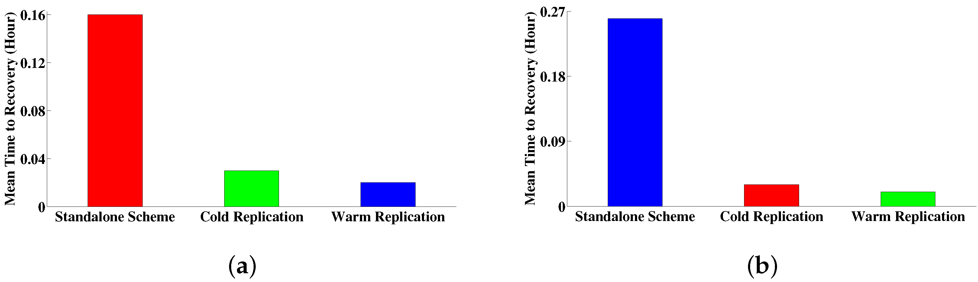
5.1.2. Failure Recovery Time

The system enters state 1 by a VM failure and while it goes into state 2 by a PM failure. Assume $T_{rv}$ and $T_{rp}$ be the mean failure recovery time for VM and PM respectively. Let $T_r$ be the combined mean failure recovery time. Refer to [26], $T_{rv}$, $T_{rp}$ and $T_r$ can be expressed by

$$\begin{array}{cc}\hfill T_{rv}& =a\left(\frac{1}{{\delta }_{vm}}+\frac{1}{{\tau }_{rb}}\right)+(1-a)\left(\frac{1}{{\delta }_{vm}}+\frac{1}{{\tau }_{rb}}+\frac{1}{{\tau }_{pv}}\right)\hfill \\ \hfill T_{rp}& =\frac{1}{{\delta }_{pm}}+\frac{1}{{\tau }_{pv}}\hfill \\ \hfill T_r& =\frac{{\gamma }_{vm}}{{\gamma }_{vm}+{\gamma }_{pm}}\left[T_{rv}\right]+\frac{{\gamma }_{pm}}{{\gamma }_{vm}+{\gamma }_{pm}}\left[T_{rp}\right]\hfill \end{array}$$

where ${\gamma }_{vm}/({\gamma }_{vm}+{\gamma }_{pm})$ is the probability of VM failure and ${\gamma }_{pm}/({\gamma }_{vm}+{\gamma }_{pm})$ is the probability of PM failure.

5.1.3. Energy Consumption Measurement

The completion time includes the downtime caused by failures. CPU utilization during the recovery time is different from that during the execution time. Thus, we need to deduct the recovery time from the completion time in order to get the actual execution time. First we need to determine the mean number of VM or PM failure occurs during the execution of a job. Let $F_{pm}$ and $F_{vm}$ be the frequency (mean number) of PM and VM failures during the execution of a job with a given work requirement.

$F_{pm}$ and $F_{vm}$ are represented by

$$\begin{array}{cc}\hfill F_{pm}& ={\gamma }_{pm}{T}_{ac}\hfill \end{array}$$

(14)

$$\begin{array}{cc}\hfill F_{vm}& ={\gamma }_{vm}{T}_{ac}\hfill \end{array}$$

(15)

The actual execution time $T_{ac}$ is

$$\begin{array}{cc}\hfill T_{ac}& =T_c-F_{vm}{T}_{rv}-F_{pm}{T}_{rp}\hfill \\ & =T_c-({\gamma }_{vm}{T}_{rv}+{\gamma }_{pm}{T}_{rp})T_{ac}\hfill \\ & =\frac{T_c}{1+{\gamma }_{vm}{T}_{rv}+{\gamma }_{pm}{T}_{rp}}\hfill \end{array}$$

VM provisioning is required when a VM fails or a PM fails, while PM provisioning is required when a PM fails. In this scheme, if VM recovery is done by rebooting the VM upon the occurrence of a VM failure, then VM provisioning is not necessary. Otherwise, the job is migrated to another PM and VM provisioning is started. We take into account the energy consumption for these scenarios accordingly. Let $N_{pm}$ and $N_{vm}$ be the mean number of PM and VM provisioning required for completing the execution of a job with a given work requirement respectively.

$$\begin{array}{cc}\hfill N_{vm}=N_{pm}& =F_{pm}+(1-a)F_{vm}+1\hfill \end{array}$$

A PM is active even if a VM fails and is ready to provision a VM. During the VM failure detection and recovery period a PM is active, hence we need to take into account the energy consumption for this period of time. In this replication scheme, the energy consumption for the VM detection and recovery scenario in the primarily deployed PM needs to be considered.

There is no standby for job execution or the server, and VM is not kept into sleep mode. Therefore, energy consumption in the standalone scheme is given by

$$\begin{array}{cc}\hfill E=E_{pr}& =P_{ac}{T}_{ac}+N_{pm}{P}_{pm}{T}_{pm}+N_{vm}{P}_{vm}{T}_{vm}+F_{vm}{P}_{vm}(\frac{1}{{\delta }_{vm}}+a\frac{1}{{\tau }_{rb}})\hfill \end{array}$$

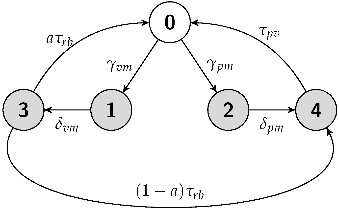
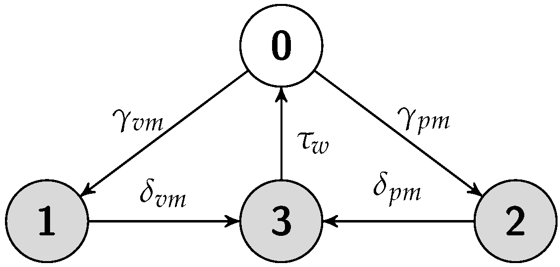
5.2. Cold Replication Scheme

We present the CTMC for the cold replication scheme as shown in Figure 2. State 0 represents the state that both the primary and the standby systems are UP and both the primary and the standby VMs are successfully provisioned where only the primary is executing the job. Any of them can fail with rates ${\gamma }_{vm}$ for VM failures and ${\gamma }_{pm}$ for PM failures. If the primary VM fails, the system enters state 1, in which it is not able to execute the job, i.e., unavailable. The unavailability in state 1 is not observable until the failure is detected. The failure is detected at the rate ${\delta }_{vm}$ upon which the system enters state 3. In this state, we perform failover and the standby assumes the role of primary (system enters state 5) and restarts the execution. The failover time is assumed to be exponentially distributed with rate ${\tau }_c$. In the meantime, provisioning of a backup VM is started on another PM at the rate ${\tau }_{pv}$ and the system returns to state 0.

The primary PM may fail at the rate ${\gamma }_{pm}$ upon which the system goes to state 2. A PM failure (system in state 2) is detected at the rate ${\delta }_{pm}$ and the system transits to state 4. As in the case of primary VM failure, the standby is switched to primary bringing the system in state 5. A new backup is started with rate ${\tau }_{pv}$ on an available node and the system returns to state 0.

In this model, standby VM does not execute the job and no execution state is copied from primary to it. It is kept ready so that it can immediately take the role of primary if there is any failure of primary. Standby VM is in deep sleep mode where the probability of VM failure in this mode is negligible. Thus, no standby VM failure is considered; only the underlying standby PM failure causes the standby VM to fail.

In case of standby PM failure, the model traverses in a similar manner as in the case of primary PM failure except the transition of switchover. If it fails, the system transits to state 6 and after detecting the PM failure with rate ${\delta }_{pm}$, the system is in state 5. In state 5, a new backup is started on an available node and the system returns to state 0.

5.2.1. Job Completion Time Computation

For completion time distribution we reduce the model shown in Figure 2. Standby PM failure-recovery and backup provisioning do not have any impact for executing jobs. Thus, we use the approximated CTMC model for cold replication scheme as shown in Figure 3.

The sojourn time distribution for each state of the CTMC in Figure 3 is given by

$$\begin{array}{cc}\hfill Q_{01}\left(t\right)& =\frac{{\gamma }_{vm}}{{\gamma }_{vm}+{\gamma }_{pm}}(1-e^{-({\gamma }_{vm}+{\gamma }_{pm})t})\hfill \\ \hfill Q_{02}\left(t\right)& =\frac{{\gamma }_{pm}}{{\gamma }_{vm}+{\gamma }_{pm}}(1-e^{-({\gamma }_{vm}+{\gamma }_{pm})t})\hfill \\ \hfill Q_{13}\left(t\right)& =Q_1\left(t\right)=1-e^{-{\delta }_{vm}t}\hfill \\ \hfill Q_{23}\left(t\right)& =Q_2\left(t\right)=1-e^{-{\delta }_{pm}t}\hfill \\ \hfill Q_{30}\left(t\right)& =Q_3\left(t\right)=1-e^{-{\tau }_{c}t}\hfill \\ \hfill Q_0\left(t\right)& =Q_{01}\left(t\right)+Q_{02}\left(t\right)=1-e^{-({\gamma }_{vm}+{\gamma }_{pm})t}\hfill \end{array}$$

Similar to standalone scheme, in this model system can execute a job only in state 0 and the work processing rate is 1 ($r_0=1$). In all other other states, the work processing rate is 0 ($r_1=r_2=r_3=0$) because the system cannot execute the job. In this scheme, the interrupted job needs to be restarted from the beginning as in the standalone scheme. Therefore, all the states are categorized in the set of $S_2$. The LST representing the time spent in the set $S_2$ obtained by Equation (9) are given by

$$\begin{array}{cc}\hfill \widetilde{M_{12,0}}(s,x)& =e^{-(s+{\gamma }_{vm}+{\gamma }_{pm})x}\hfill \\ & +\frac{{\gamma }_{vm}}{s+{\gamma }_{vm}+{\gamma }_{pm}}(1-e^{-(s+{\gamma }_{vm}+{\gamma }_{pm})x})\widetilde{M_{12,1}}(s,x)\hfill \\ & +\frac{{\gamma }_{pm}}{s+{\gamma }_{vm}+{\gamma }_{pm}}(1-e^{-(s+{\gamma }_{vm}+{\gamma }_{pm})x})\widetilde{M_{12,2}}(s,x)\hfill \\ \hfill \widetilde{M_{12,1}}(s,x)& =\frac{{\delta }_{vm}}{s+{\delta }_{vm}}\widetilde{M_{12,3}}(s,x)\hfill \\ \hfill \widetilde{M_{12,2}}(s,x)& =\frac{{\delta }_{pm}}{s+{\delta }_{pm}}\widetilde{M_{12,3}}(s,x)\hfill \\ \hfill \widetilde{M_{12,3}}(s,x)& =\frac{{\tau }_c}{s+{\tau }_c}\widetilde{M_{12,0}}(s,x)\hfill \end{array}$$

Similar to standalone scheme, we get the mean job completion time.

5.2.2. Failure Recovery Time

$T_{rv}$, $T_{rp}$ and $T_r$ in Figure 3 are given by

$$\begin{array}{cc}\hfill T_{rv}& =\frac{1}{{\delta }_{vm}}+\frac{1}{{\tau }_c}\hfill \\ \hfill T_{rp}& =\frac{1}{{\delta }_{pm}}+\frac{1}{{\tau }_c}\hfill \\ \hfill T_r& =\frac{{\gamma }_{vm}}{{\gamma }_{vm}+{\gamma }_{pm}}\left[T_{rv}\right]+\frac{{\gamma }_{pm}}{{\gamma }_{vm}+{\gamma }_{pm}}\left[T_{rp}\right]\hfill \end{array}$$

5.2.3. Energy Consumption Measurement

We have the mean job completion time, $T_c$ and the mean failure recovery times for PM and VM. The frequencies of PM failures and VM failures are computed as $F_{pm}$ and $F_{vm}$ using Equations (14) and (15) respectively. The actual execution time is

$$\begin{array}{cc}\hfill T_{ac}& =\frac{T_c}{1+{\gamma }_{vm}{T}_{rv}+{\gamma }_{pm}{T}_{rp}}\hfill \end{array}$$

The mean number of PM provisioning is $N_{pm}=F_{pm}+1$ for primary and standby PM. The mean number of VM provisioning in primary is $N_{v{m}_{pr}}=F_{vm}+F_{pm}+1$. For standby VM, the mean number of VM provisioning is equal to $N_{pm}$ and hence $N_{v{m}_{st}}=N_{pm}=F_{pm}+1$.

In addition, we need to estimate the amount of time standby lies in sleep mode. In cold replication a standby is in sleep mode except the failover and backup provisioning time. When a standby takes over as primary or when a standby PM fails, a backup is being provisioned and kept in sleep mode. Backup provisioning is done in the background, while the job is being executed by primary. Therefore,

$$\begin{array}{c}\hfill T_{dsp}=T_c-(F_{vm}+F_{pm})\frac{1}{{\tau }_c}\end{array}$$

PM provisioning mode. Generally, in cold and warm replication scheme, no individual PM solely works as primary or standby. In particular, every individual PM hosts the primary VM for some jobs while it hosts the standby VM for some other jobs. Thus, PM provisioning mode power consumption in standby PM need not to take into account for this individual job, because power consumption of this mode is considered by some other jobs for which this standby PM works as primary.

Similar to the standalone scheme, we take into account the energy consumption of PM during the VM detection and recovery period. The energy consumption in cold replication scheme is given by

$$\begin{array}{cc}\hfill E& =E_{pr}+E_{st}\hfill \end{array}$$

where

$$E_{pr}=P_{ac}{T}_{ac}+N_{pm}{P}_{pm}{T}_{pm}+N_{v{m}_{pr}}{P}_{vm}{T}_{vm}+F_{vm}{P}_{vm}{T}_{rv}$$

and

$$E_{st}=N_{v{m}_{st}}{P}_{vm}{T}_{vm}+P_{dsp}{T}_{dsp}$$

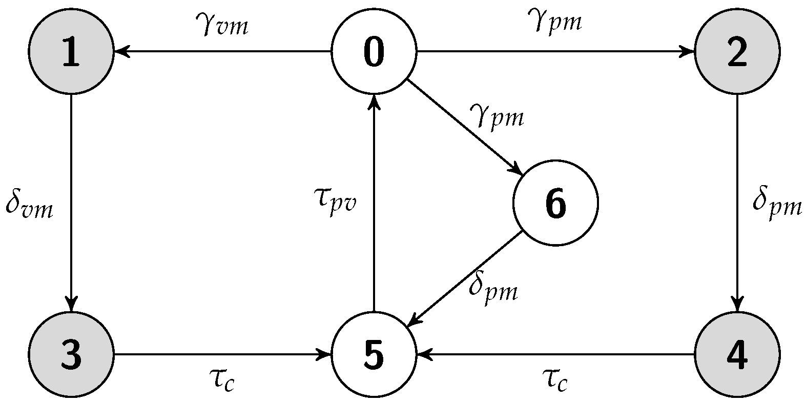
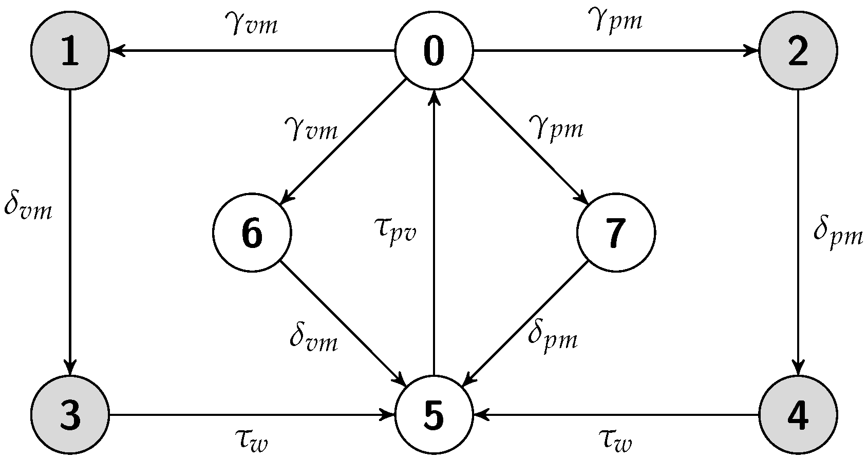
5.3. Warm Replication Scheme

Figure 4 shows the CTMC for warm replication scheme. State 0 represents the state that both the primary and the standby systems are UP and both the primary and the standby VMs are successfully provisioned where only the primary is executing the job. Any of the VMs or PMs can fail with rates ${\gamma }_{vm}$ for VM failures and ${\gamma }_{pm}$ for PM failures. If the primary VM fails, the system enters state 1, in which it is not able to execute the job, i.e., unavailable. The failure is detected at the rate ${\delta }_{vm}$ upon which the system enters state 3. In this state, we perform failover and the standby assumes the role of primary (system enters state 5). The failover time is assumed to be exponentially distributed with rate ${\tau }_w$. In the meantime, provisioning of a backup VM is started on another PM at the rate ${\tau }_{pv}$ and the system returns to state 0.

The primary PM may fail at the rate ${\gamma }_{pm}$ upon which the system goes to state 2 and is unavailable. After detection of PM failure with rate ${\delta }_{pm}$, the system transits to state 4. In state 4 (as in the case of primary VM failure), the standby PM is switched to primary bringing the system in state 5. A new backup is started on an available node and the system returns to state 0.

In case of standby VM failure, upon which the system is in state 6, the primary is still executing the job. After the standby VM failure detection with rate ${\delta }_{vm}$ (system is in state 5), a VM is provisioned on another PM with rate ${\tau }_{pv}$ and the system returns to state 0.

In case of standby PM failure, the model traverses in a similar manner as in the case of primary PM failure except the transition of switchover. If it fails, system transits to state 7 and after detecting the failure system is in state 5. In state 5, a new backup is started on an available node and the system returns to state 0.

5.3.1. Job Completion Time Computation

For completion time distribution we reduce the model shown in Figure 4, because we have difficulty in taking the numerical inversion of Laplace Transform for the analysis of structure-state process. In addition, standby failure-repair and backup provisioning do not have any impact for executing jobs. Thus, we use the approximated CTMC model for warm replication scheme as shown in Figure 5.

The sojourn time distribution of the states are given by

$$\begin{array}{cc}\hfill Q_{01}\left(t\right)& =\frac{{\gamma }_{vm}}{{\gamma }_{vm}+{\gamma }_{pm}}(1-e^{-({\gamma }_{vm}+{\gamma }_{pm})t})\hfill \\ \hfill Q_{02}\left(t\right)& =\frac{{\gamma }_{pm}}{{\gamma }_{vm}+{\gamma }_{pm}}(1-e^{-({\gamma }_{vm}+{\gamma }_{pm})t})\hfill \\ \hfill Q_{13}\left(t\right)& =Q_1\left(t\right)=1-e^{-{\delta }_{vm}t}\hfill \\ \hfill Q_{23}\left(t\right)& =Q_2\left(t\right)=1-e^{-{\delta }_{pm}t}\hfill \\ \hfill Q_{30}\left(t\right)& =Q_3\left(t\right)=1-e^{-{\tau }_{w}t}\hfill \\ \hfill Q_0\left(t\right)& =Q_{01}\left(t\right)+Q_{02}\left(t\right)=1-e^{-({\gamma }_{vm}+{\gamma }_{pm})t}\hfill \end{array}$$

In this model, all the states are in the set of $S_1$ and the work processing rate of the states are $r_0=1$ and $r_1=r_2=r_3=0$ respectively. The LST double transforms representing the times spent in the set $S_1$ obtained by Equation (7) are given by

$$\begin{array}{cc}\hfill \widetilde{M_{1,0}^{*}}(s,w)& =\frac{1}{s+w+{\gamma }_{vm}+{\gamma }_{pm}}\hfill \\ & +\frac{{\gamma }_{vm}}{s+w+{\gamma }_{vm}+{\gamma }_{pm}}\widetilde{M_{1,1}^{*}}(s,w)\hfill \\ & +\frac{{\gamma }_{pm}}{s+w+{\gamma }_{vm}+{\gamma }_{pm}}\widetilde{M_{1,2}^{*}}(s,w)\hfill \\ \hfill \widetilde{M_{1,1}^{*}}(s,w)& =\frac{{\delta }_{vm}}{s+{\delta }_{vm}}\widetilde{M_{1,3}^{*}}(s,w)\hfill \\ \hfill \widetilde{M_{1,2}^{*}}(s,w)& =\frac{{\delta }_{pm}}{s+{\delta }_{pm}}\widetilde{M_{1,3}^{*}}(s,w)\hfill \\ \hfill \widetilde{M_{1,3}^{*}}(s,w)& =\frac{{\tau }_w}{s+{\tau }_w}\widetilde{M_{1,0}^{*}}(s,w)\hfill \end{array}$$

By performing inverse Laplace transform of $\widetilde{M_{1,0}^{*}}(s,w)$, with respect to w (the correspondence of x), we get $\widetilde{M_{1,0}}(s,x)$. Similarly, we get $\widetilde{M_{1,1}}(s,x)$, $\widetilde{M_{1,2}}(s,x)$ and $\widetilde{M_{1,3}}(s,x)$.

Similar to standalone and cold replication scheme, we get the mean job completion time.

5.3.2. Failure Recovery Time

$T_{rv}$, $T_{rp}$ and $T_r$ in Figure 5 are given by

$$\begin{array}{cc}\hfill T_{rv}& =\frac{1}{{\delta }_{vm}}+\frac{1}{{\tau }_w}\hfill \\ \hfill T_{rp}& =\frac{1}{{\delta }_{pm}}+\frac{1}{{\tau }_w}\hfill \\ \hfill T_r& =\frac{{\gamma }_{vm}}{{\gamma }_{vm}+{\gamma }_{pm}}\left[T_{rv}\right]+\frac{{\gamma }_{pm}}{{\gamma }_{vm}+{\gamma }_{pm}}\left[T_{rp}\right]\hfill \end{array}$$

5.3.3. Energy Consumption Measurement

We have the mean job completion time, $T_c$ as well as the mean failure recovery time for PM and VM. We get the values of $F_{pm}$ and $F_{vm}$ using Equations (14) and (15) respectively and the values of $N_{pm}=F_{pm}+1$ and $N_{vm}=F_{vm}+F_{pm}+1$. The actual execution time is

$$\begin{array}{cc}\hfill T_{ac}& =\frac{T_c}{1+{\gamma }_{vm}{T}_{rv}+{\gamma }_{pm}{T}_{rp}}\hfill \end{array}$$

The time spent in sleep mode by standby is

$$\begin{array}{c}\hfill T_{lsp}=T_c-(F_{vm}+F_{pm})\frac{1}{{\tau }_w}\end{array}$$

Similar to standalone and cold replication scheme, we take into account the energy consumption of PM during the VM detection and recovery period. The energy consumption in a warm replication scheme is given by

$$\begin{array}{cc}\hfill E& =E_{pr}+E_{st}\hfill \end{array}$$

where

$$E_{pr}=P_{ac}{T}_{ac}+N_{pm}{P}_{pm}{T}_{pm}+N_{vm}{P}_{vm}{T}_{vm}+F_{vm}{P}_{vm}{T}_{rv}$$

and

$$E_{st}=N_{vm}{P}_{vm}{T}_{vm}+P_{lsp}{T}_{sp}+F_{vm}{P}_{vm}\frac{1}{{\delta }_{vm}}$$

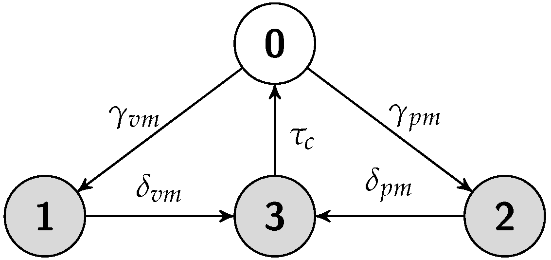
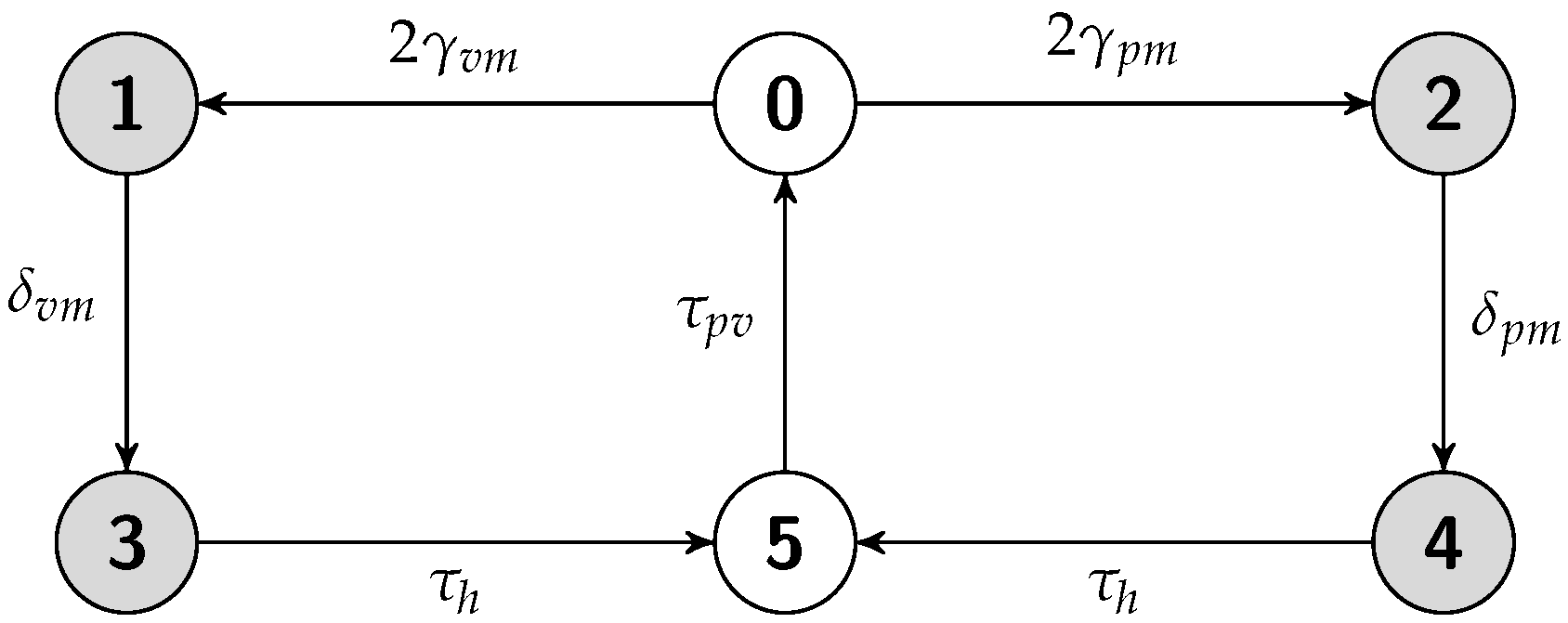
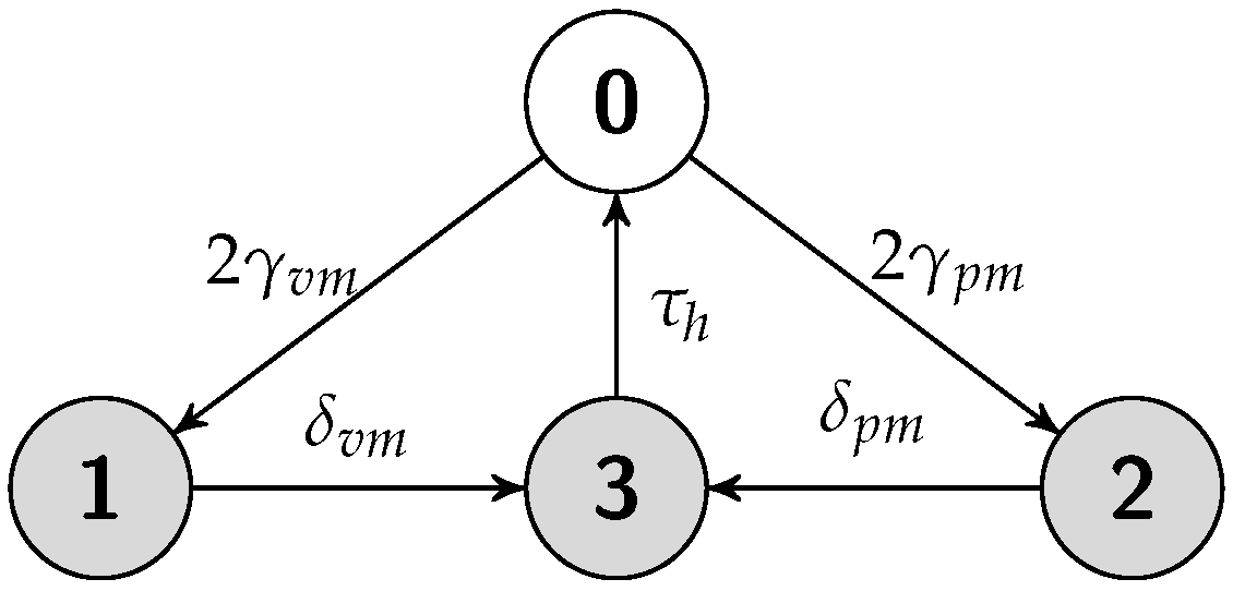
5.4. Hot Replication Scheme

Figure 6 shows the CTMC for hot replication scheme. State 0 represents the state that both the primary and the standby systems are UP and both the primary and the standby VMs execute the same job in parallel. Any of the VMs or PMs can fail with rates ${\gamma }_{vm}$ for VM failures and ${\gamma }_{pm}$ for PM failures. If one of the VMs (either primary or standby) fails, the system enters state 1, (i.e., one VM is down). Though another VM is available, job execution is not being interrupted due to a single VM failure. The failure is detected at the rate ${\delta }_{vm}$ upon which the system enters state 3. In state 3, we perform switchover and the another (standby) VM assumes the role of primary, and system enters state 5. The switching time is assumed to be exponentially distributed with mean $1/{\tau }_h$. In the meantime, provisioning of a backup VM is started on another PM at the rate ${\tau }_{pv}$, the system goes back to state 0, and resumes the execution as in the warm replication scheme.

The PM may fail at the rate ${\gamma }_{pm}$ upon which the system goes to state 2 (i.e., one PM is down). Similar to VM failure scenario, job execution is not interrupted due to a single PM failure. On the other hand, after detection of PM failure with rate ${\delta }_{pm}$, the system transits to state 4. In state 4 (as in the case of primary VM failure), the standby PM is switched to primary bringing the system in state 5. A new backup is started on an available node to take the system back to state 0. Note that the probability of subsequent failures of both VMs or both PMs before the detection and recovery of another one are negligible [26]. Thus, job interruption probability is also negligible in this scheme.

5.4.1. Job Completion Time Computation

For completion time distribution we reduce the model shown in Figure 6. Similar to the warm replication scheme, we use the approximated CTMC model for hot replication scheme as shown in Figure 7.

The sojourn time distributions of the states are given by

$$\begin{array}{cc}\hfill Q_{01}\left(t\right)& =\frac{{\gamma }_{vm}}{{\gamma }_{vm}+{\gamma }_{pm}}(1-e^{-(2{\gamma }_{vm}+2{\gamma }_{pm})t})\hfill \\ \hfill Q_{02}\left(t\right)& =\frac{{\gamma }_{pm}}{{\gamma }_{vm}+{\gamma }_{pm}}(1-e^{-(2{\gamma }_{vm}+2{\gamma }_{pm})t})\hfill \\ \hfill Q_{13}\left(t\right)& =Q_1\left(t\right)=1-e^{-{\delta }_{vm}t}\hfill \\ \hfill Q_{23}\left(t\right)& =Q_2\left(t\right)=1-e^{-{\delta }_{pm}t}\hfill \\ \hfill Q_{30}\left(t\right)& =Q_3\left(t\right)=1-e^{-{\tau }_{h}t}\hfill \\ \hfill Q_0\left(t\right)& =Q_{01}\left(t\right)+Q_{02}\left(t\right)=1-e^{-(2{\gamma }_{vm}+2{\gamma }_{vm})t}\hfill \end{array}$$

In this model, all the states are in the set of $S_1$ (refer to Figure 7) and the work processing rate of the states are $r_0=r_1=r_2=r_3=1$. The LST double transforms representing the times spent in the set $S_1$ obtained by Equation (7) are given by

$$\begin{array}{cc}\hfill \widetilde{M_{1,0}^{*}}(s,w)& =\frac{1}{s+w+2{\gamma }_{vm}+2{\gamma }_{pm}}\hfill \\ & +\frac{2{\gamma }_{vm}}{s+w+2{\gamma }_{vm}+2{\gamma }_{pm}}\widetilde{M_{1,1}^{*}}(s,w)\hfill \\ & +\frac{2{\gamma }_{pm}}{s+w+2{\gamma }_{vm}+2{\gamma }_{pm}}\widetilde{M_{1,2}^{*}}(s,w)\hfill \\ \hfill \widetilde{M_{1,1}^{*}}(s,w)& =\frac{1}{s+w+{\delta }_{vm}}+\frac{{\delta }_{vm}}{s+w+{\delta }_{vm}}\widetilde{M_{1,3}^{*}}(s,w)\hfill \\ \hfill \widetilde{M_{1,2}^{*}}(s,w)& =\frac{1}{s+w+{\delta }_{pm}}+\frac{{\delta }_{pm}}{s+w+{\delta }_{pm}}\widetilde{M_{1,3}^{*}}(s,w)\hfill \\ \hfill \widetilde{M_{1,3}^{*}}(s,w)& =\frac{1}{s+w+{\tau }_h}+\frac{{\tau }_h}{s+w+{\tau }_h}\widetilde{M_{1,0}^{*}}(s,w)\hfill \end{array}$$

By performing inverse Laplace transform of $\widetilde{M_{1,0}^{*}}(s,w)$, with respect to w (the correspondence of x), we get $\widetilde{M_{1,0}}(s,x)$. Similarly, we get $\widetilde{M_{1,1}}(s,x)$, $\widetilde{M_{1,2}}(s,x)$ and $\widetilde{M_{1,3}}(s,x)$.

Similar to the standalone, cold, and warm replication scheme, we get the mean job completion time.

5.4.2. Failure Recovery Time

In the hot replication scheme, there is no interruption of job execution. However, in order to compute the actual execution time by standby, the mean time to recovery (MTTR) for VM and PM needs to be analyzed. $T_{rv}$ and $T_{rp}$ in Figure 7 are given by

$$\begin{array}{cc}\hfill T_{rv}& =\frac{1}{{\delta }_{vm}}+\frac{1}{{\tau }_h}\hfill \\ \hfill T_{rp}& =\frac{1}{{\delta }_{pm}}+\frac{1}{{\tau }_h}\hfill \end{array}$$

5.4.3. Energy Consumption Measurement

In this replication scheme, the energy consumption for the two individual copies of VMs (primary and standby) in primary and standby PMs needs to be computed since both of the copies are executing the job simultaneously.

The mean job completion time, $T_c$ is equal to the value of work requirement. $F_{pm}$ and $F_{vm}$ are derived by Equations (14) and (15) respectively and $N_{pm}=F_{pm}+1$ and $N_{vm}=F_{vm}+F_{pm}+1$.

$$\begin{array}{cc}\hfill T_{a{c}_{pr}}& =T_c\hfill \\ \hfill T_{a{c}_{st}}& =T_c-F_{pm}{T}_{rp}-F_{vm}{T}_{rv}\hfill \\ & =\frac{T_c}{1+{\gamma }_{vm}{T}_{rv}+{\gamma }_{pm}{T}_{rp}}\hfill \end{array}$$

The energy consumption in hot replication scheme is given by

$$\begin{array}{cc}\hfill E& =E_{pr}+E_{st}\hfill \end{array}$$

where

$$E_{pr}=P_{ac}{T}_{a{c}_{pr}}+N_{pm}{P}_{pm}{T}_{pm}+N_{vm}{P}_{vm}{T}_{vm}+F_{vm}{P}_{vm}{T}_{rv}$$

and

$$E_{st}=P_{ac}{T}_{a{c}_{st}}+N_{pm}{P}_{pm}{T}_{vm}+N_{vm}{P}_{vm}{T}_{vm}+F_{vm}{P}_{vm}{T}_{rv}$$

As noted above, we perform periodic mirroring of execution state and data in the warm and hot replication scheme, so the energy consumption due to the increase in CPU utilization of every individual periodic mirroring needs to be considered. The mirroring operation is IO intensive and CPU utilization is very low (on average 2% of maximum utilization) during the IO intensive job [20,21]. In addition, the migration time is short enough which varies around 1 minute [27,28]. The total energy consumption for the accumulated migration period of a job completion is marginal.

6. Experiments

To verify the validity of our proposed analytical modeling approach, we extend CloudSim [22,23] for our experiments. The following sections outline the experimental settings. We then compare the analytical modeling approach with simulation in terms of job completion time and energy consumption results. Furthermore, the results of sensitivity analysis of parameter values are presented.

6.1. CloudSim Extension

CloudSim [22,23] is a widely used extensible simulation framework that supports modeling of virtual resource allocation, job scheduling, and other functionalities. We use CloudSim in the following way to support our experiments:

• A data center network is constructed to connect the host servers that can deploy more than one VM.
• VM or PM failure, failure detection, and recovery events are triggered. An event can be generated according to a specified distribution. The failure event data and the recovery event data can be saved to a file so the experiment can be repeated.
• Power consumption module and associated time event for every individual mode of resource provisioning and servicing discussed in Section 4.1 is generated.
• A checkpoint state is generated, transferred, and stored based on the preemption of structure-state process and replication scheme. This module is extensible.
• A job is resumed from a VM failure based on the saved checkpoint state and replication scheme. If there is no accessible checkpoint state, it restarts the job from the beginning.

6.2. Experimental Setup

We construct a data center network in CloudSim in which each host server can deploy 4 VMs individually. We configure each host server and each VM in the following way:

• The miph (millions of instructions per hour) of each host server is 4,000,000, the disk size is 100 GB, the memory size is 4 GB, and the bandwidth is 4000 bps.
• The miph of each VM is 1,000,000, and the disk size is 25 GB, the memory size is 1 GB, and the bandwidth is 1000 bps.

6.3. Model Parameterization

Table 1. Default value of parameters.

Parameters	Description	Values
		Set1	Set2
u	Average CPU utilization of a single job	25%	25%
$T_{pm}$	Mean time for PM provisioning	3 min	3 min
$T_{vm}$	Mean time for VM provisioning	10 min	15 min
$P_{max}$	Power consumption at maximum utilization	0.25 KW	0.25 KW
$1/{\gamma }_{vm}$	Mean time to failure of VM (MTTF_VM)	48 h	240 h
$1/{\gamma }_{pm}$	Mean time to failure of PM (MTTF_PM)	192 h	720 h
$1/{\delta }_{vm}$	Mean time for failure detection of VM	2 s	2 s
$1/{\delta }_{pm}$	Mean time for failure detection of PM	5 s	5 s
$1/{\tau }_{rb}$	Mean time for VM recovery by rebooting	5 min	5 min
$1/{\tau }_{pv}$	Mean time for VM provisioning in a new PM	15 min	30 min
a	Coverage factor of VM recovery by rebooting	0.80	0.80
$1/{\tau }_c$	Mean time for failover in cold replication	2 min	2 min
$1/{\tau }_w$	Mean time for failover in warm replication	1 min	1 min
$1/{\tau }_h$	Mean time for switchover in hot replication	15 s	30 s
x	Amount of work requirements	50 unit	300 unit

shows the default parameter values used in the experiments. Two different sets of values are used. The values of Set1 proposed by us and with reference to [1,7,15], and Set2 by [1,7,12,15]. We take the reference of Figure 5.15 [7] for considering the mean time for VM recovery and provisioning in different replication schemes. The work processing rates of every individual states of CTMC are measured by $[unit/hour]$ where processing rate 1 means 1,000,000 miph which is equal to the miph of each VM in the UP state.

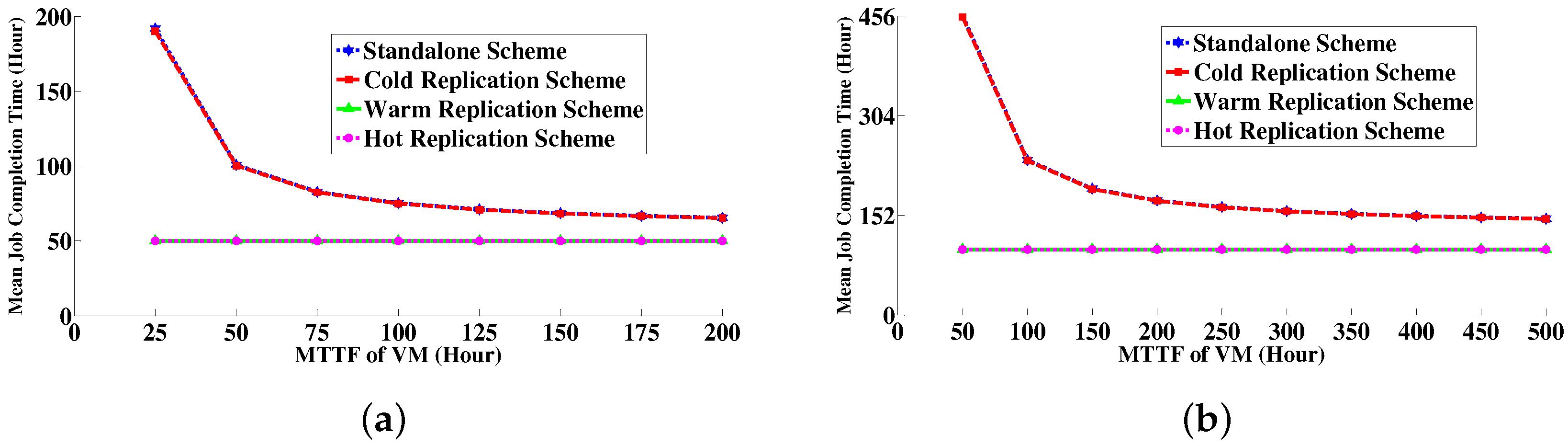
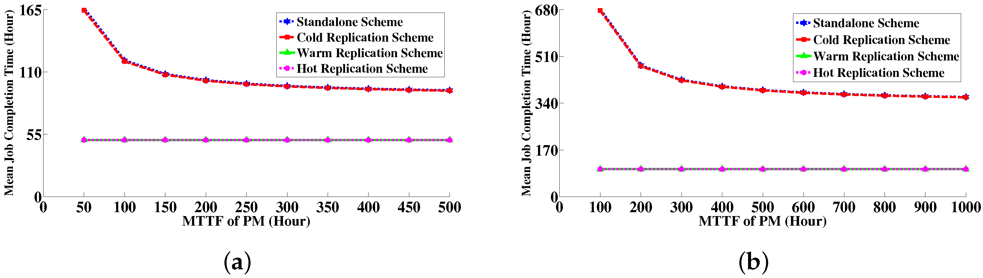
6.4. Numerical Results

This section provides the numerical results to present the impacts of replication schemes on transient availability, job completion time, and energy consumption based on the formulation derived in the previous section. Note that we show the computation for both sets of parameter values side by side. Any deviations from these parameter values are explicitly noted.

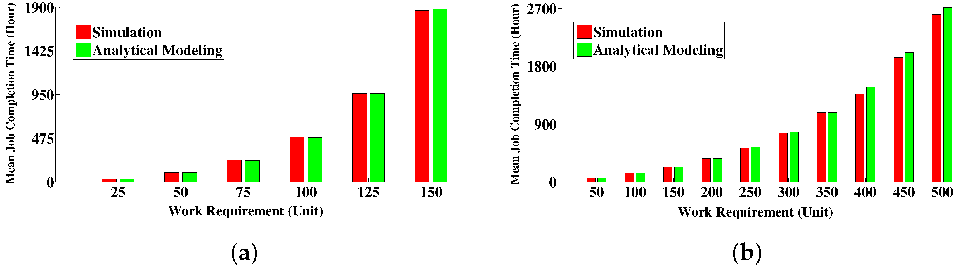
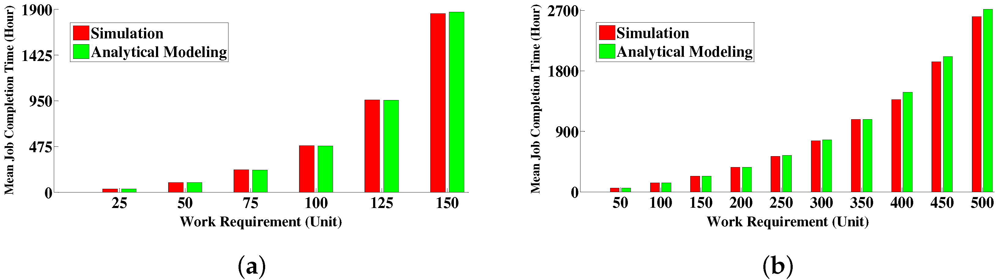
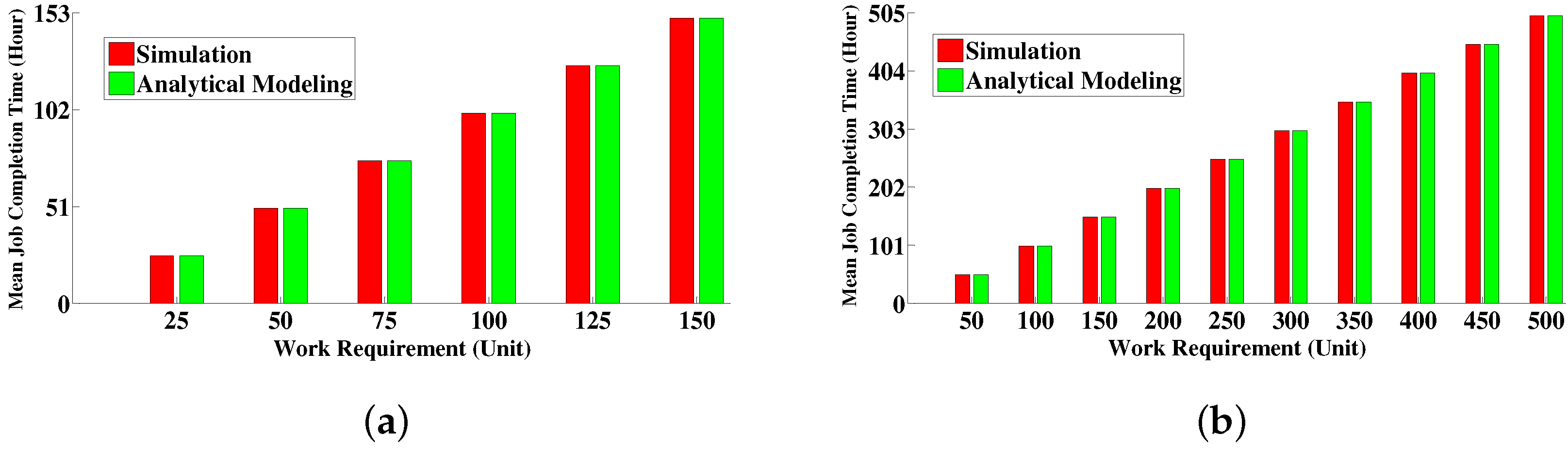
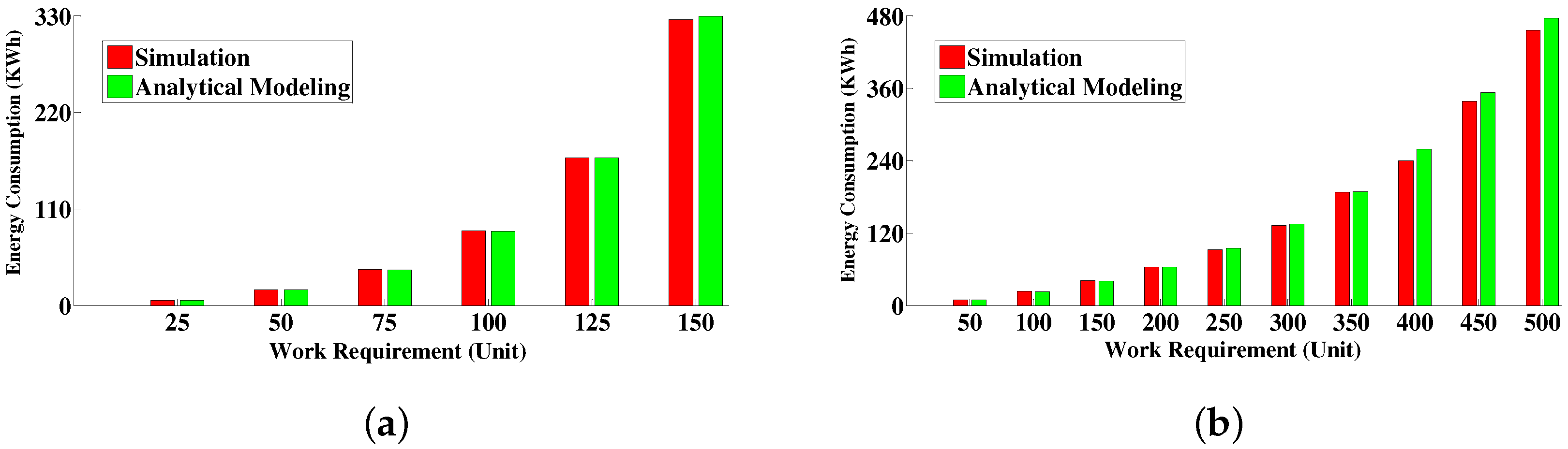
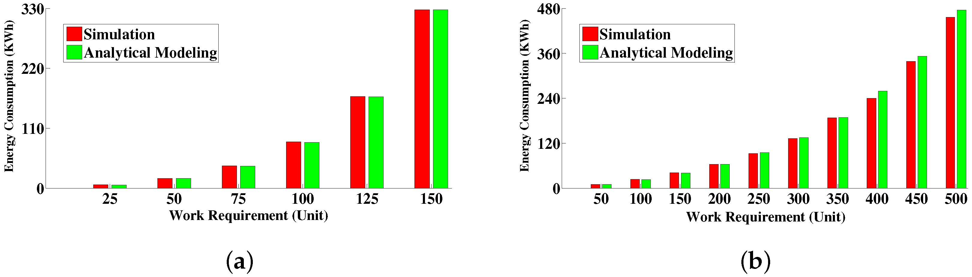
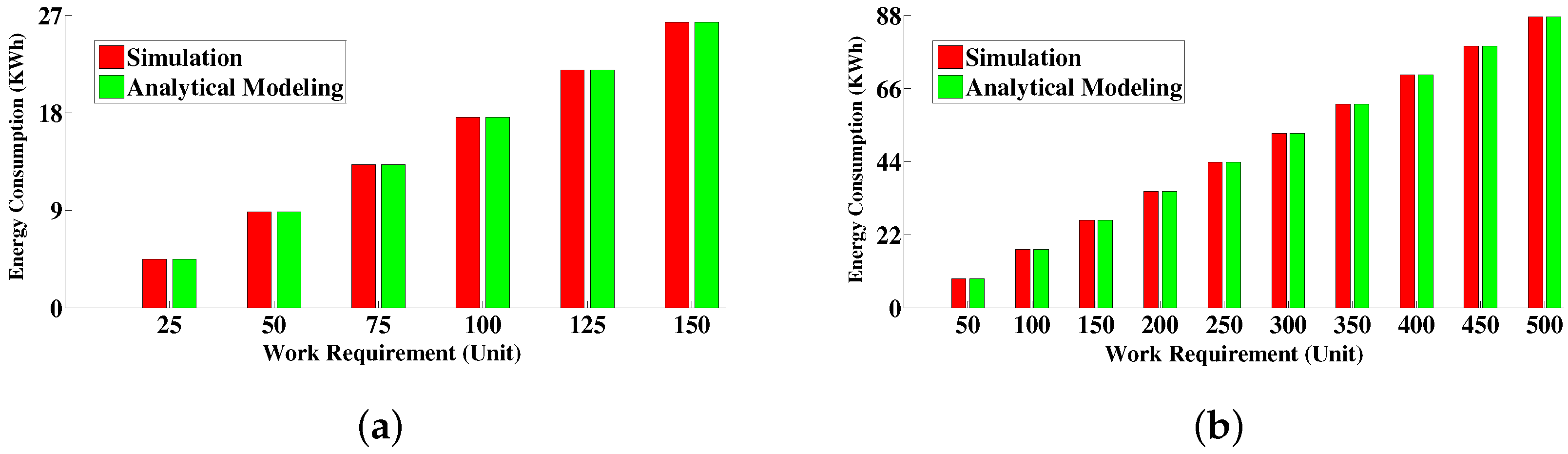
6.4.1. Comparison between Simulative Solution and Analytical Modeling Solution

In our simulation the sample size for every individual execution is 1,000,000.

In Figure 8, Figure 9 and Figure 10 we show the comparison of mean job completion time between simulative solution and analytic modeling solution in standalone, cold, and warm replication schemes respectively. We show the computation with different work requirements for both sets of parameter values. In standalone and cold replication scheme, the difference in completion time between these two approaches is negligible when the work requirement is less than the MTTF or around (either VM or PM which one is smaller, here MTTF of VM is smaller than PM and it is 48 h in Set1, 240 h in Set2), but beyond that the difference increases gradually. On the other hand, in warm replication the difference is negligible for any value of work requirement. Note that we do not show the comparison between simulative solution and analytical modeling solution for hot replication. As noted above, there is no interruption of execution in this scheme, so job completion time would be equal to the numeric value of work requirement both by simulative solution and analytical modeling solution, as well as expected energy consumption would be same consequently.

In

Table 2. Ninety-Five Percent Confidence Interval of job completion time computed by simulation.

Work Requirement	95% Confidence Interval of Job Completion Time (Hour)
	Standalone Scheme (Set1)			Cold Replication (Set1)			Warm Replication (Set1)
	Lower Limit	Mean	Upper Limit	Lower Limit	Mean	Upper Limit	Lower Limit	Mean	Upper Limit
25	35.266	35.3728	35.4795	35.1995	35.3057	35.4119	25.0102	25.0103	25.0104
50	103.5778	104.0084	104.439	102.8789	103.3031	103.7273	50.0200	50.0201	50.0202
75	234.8593	236.0109	237.1626	233.8017	234.9451	236.0886	75.0293	75.0295	75.0296
100	482.0843	485.7264	487.2298	484.2511	486.8565	489.4619	100.0381	100.0383	100.0385
125	958.0949	961.1457	969.0413	956.1904	961.6283	967.0663	125.0462	125.0465	125.0468
150	1847.4	1855.8326	1869.2	1840.1	1850.9	1861.7	150.0538	150.0541	150.0545

, we show the 95% confidence interval of job completion time computed by simulation in standalone, cold, and warm replication scheme for first set of parameter values. The lower limits and the upper limits are in close agreement with the means. In standalone and cold replication, the difference between the upper limit and lower limit increases gradually as the work requirement increases. On the other hand, the difference in warm replication is negligible for any value of work requirement.

Figure 11 shows the mean job completion time and its standard deviation obtained from simulation in standalone, cold, and warm replication scheme separately. The standard deviations are plotted in both sides around the mean values by filled rectangles. In standalone and cold replication, mean job completion time as well as its standard deviation increases rapidly as the work requirement increases. On the other hand, in warm replication, job completion time increases a bit as the work requirement increases and its standard deviation is a negligible value.

In Figure 12, Figure 13 and Figure 14, we show the comparison of expected energy consumption between simulative solution and analytic modeling solution in standalone, cold, and warm replication schemes respectively. The graphs behave similarly as the job completion time in Figure 8, Figure 9 and Figure 10.

Figure 15 shows the mean job completion time for the replication schemes combinedly in order to make a clear distinction among them. The difference in job completion time between standalone and cold replication scheme is very much short (For example, $x=50$ and Set1 parameter values, $T_c$ in standalone scheme $=103.216$ and in cold replication $=102.886$ h). The time is larger in standalone scheme due to larger recovery time Recovery times in different replication schemes are shown in Figure 16 than in cold replication scheme, because of the absence of any redundant copy of VM or VM instances therein. In cold replication scheme if the primary fails, we activate the suspended standby which takes short time for recovery than in standalone scheme. The job completion time in standalone and cold replication scheme is comparatively much higher than in warm and hot replication scheme, because in these two schemes we need to restart the job every time upon the occurrence of a failure and rises rapidly especially if the work requirement is greater than the MTTF (as discussed before). On the other hand, in warm replication we can resume the job execution in recovery process and the time for activating the paused standby VM is comparatively quite short [7]. Consequently, the mean job completion time with warm replication is much shorter than standalone and cold replication case regardless of the amount of work requirements.

Further, the completion time in warm and hot replication schemes are almost same; have a little negligible difference. In warm replication, only primary executes the job and unidirectional periodical mirroring from primary to standby is observed. On the other hand, in hot replication there is bidirectional mirroring between primary and standby and both the primary and standby execute the same job as well. Failover/switchover time is less in hot replication than in warm replication and a single failure (whether VM or PM) in hot replication does not have any impact for executing the job [26]. Thus, it takes less time in hot replication to complete the execution upon the occurrence of a failure. In particular, completion time in a hot replication scheme is equal to numeric value of work requirement.

In Figure 17, we show the mean job completion time by varying the MTTF of VM. We show the computation for two different work requirements, $x=50$ and $x=100$ in the replication schemes considering the first set of parameter values. Mean job completion time in warm replication scheme improves a bit as the MTTF increases and does not vary in hot replication though there is no interruption in execution. On the other hand, in standalone and cold replication schemes, the completion time decreases gradually as MTTF increases. This is because, in warm replication scheme, we can resume the execution of the failed job upon recovery, thereby the job completion does not vary significantly. On the other hand, in standalone and cold replication scheme, we need to restart the failed job upon recovery and as the MTTF increases, the frequency of failure decreases, consequently resulting in the improvement of completion time. Further, as can be noticed, completion time improves a bit after a certain MTTF value (175 in Figure 17a, and 450 in Figure 17b).

Similar to Figure 17, we show the mean job completion time by varying the MTTF of PM in Figure 18. The graphs behave similarly as in Figure 17.

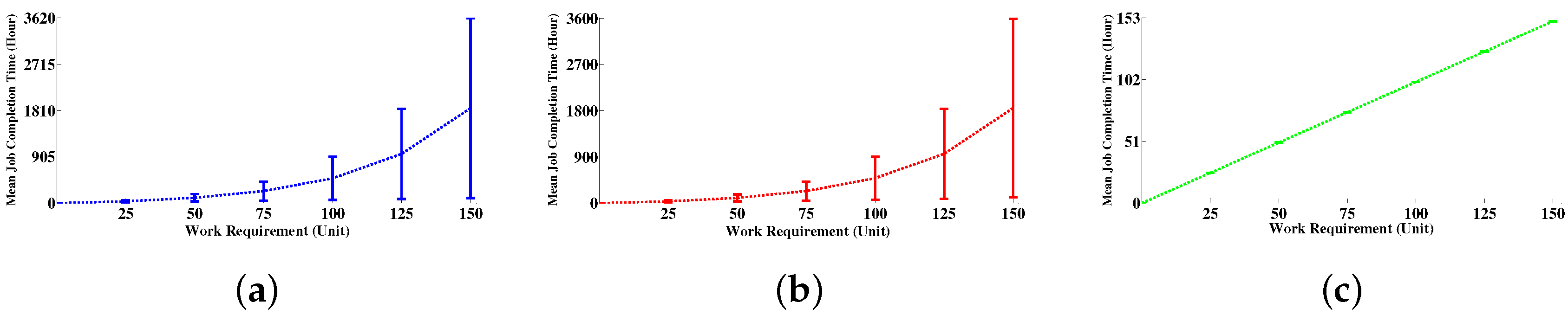
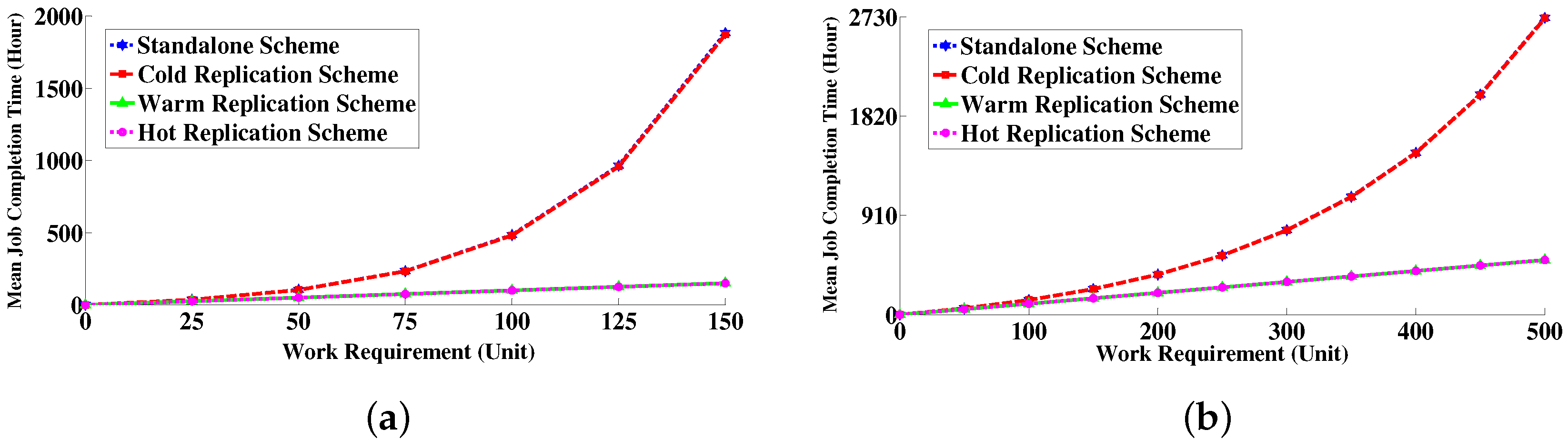
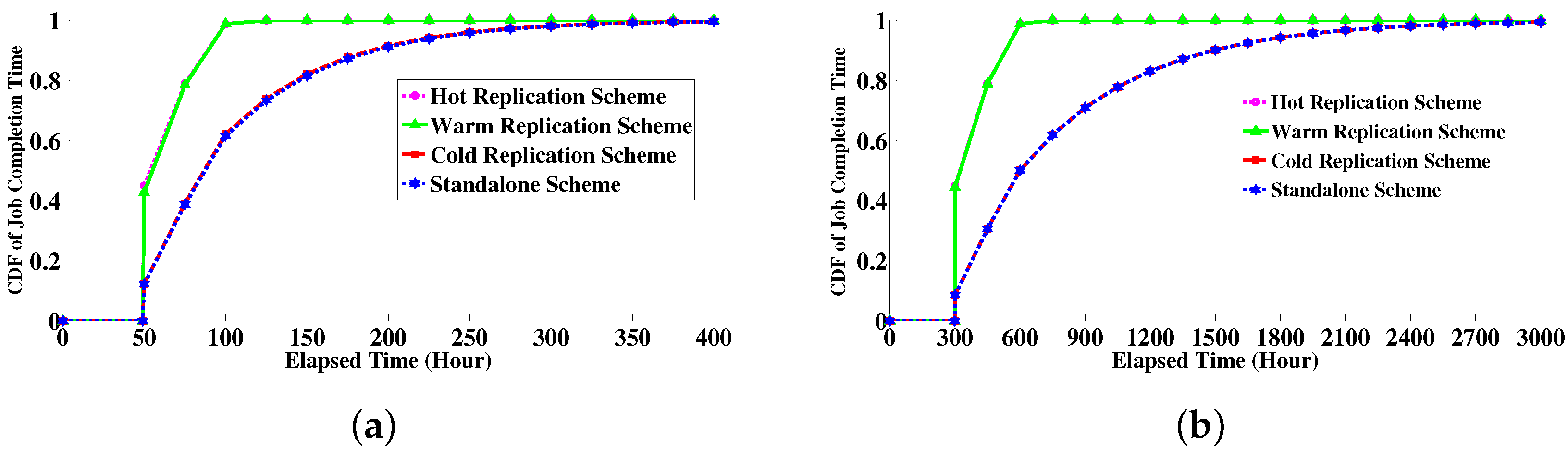
6.4.2. Job Completion Time Distribution

In Figure 19, we show the CDF of job completion time for the replication schemes. If the system (either VM or PM) does not encounter any failures for 50 h, the job execution completes at $t=50$ (work requirement is 50 units for the computation in Figure 19a. Similarly, if the system (either VM or PM) does not encounter any failures for 300 h, the job execution completes at $t=300$ (work requirement is 300 units for the computation in Figure 19b). Further, the probability of job completion in standalone and cold replication scheme approaching 1 is slower than in the warm and hot replication scheme, because we cannot save the execution states of jobs, but in warm replication scheme we can resume the execution upon failure recovery as well as in hot replication scheme we can resume the execution upon failure recovery and there is no interruption in execution. In addition, the difference between warm and hot replication scheme comes from the downtime overhead in warm replication and the difference is negligible.

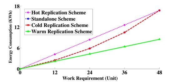
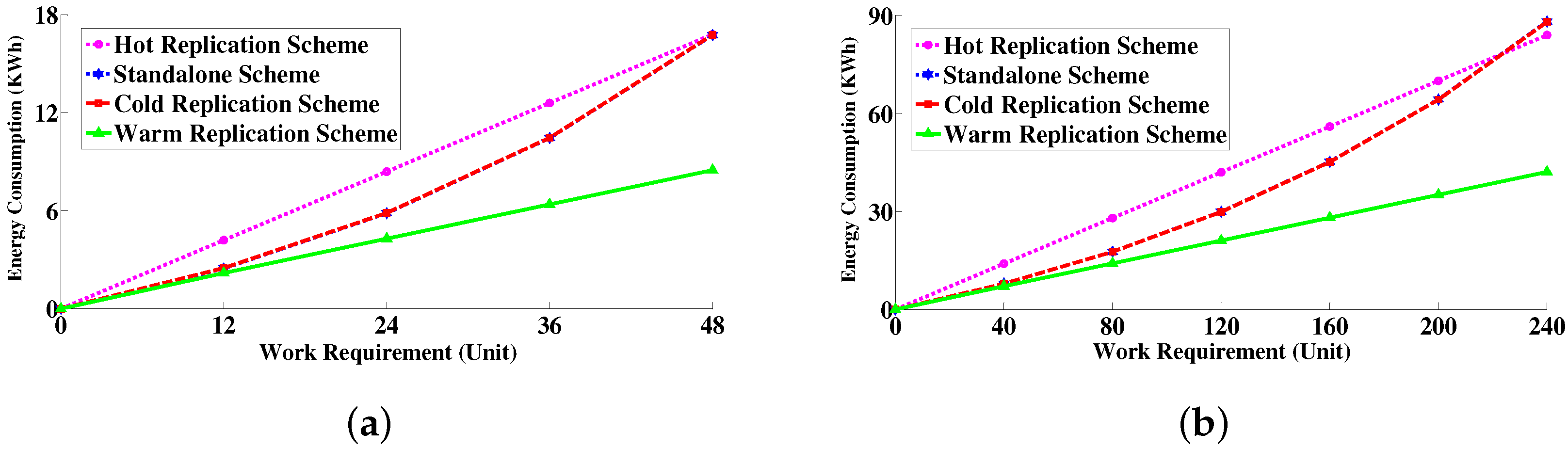
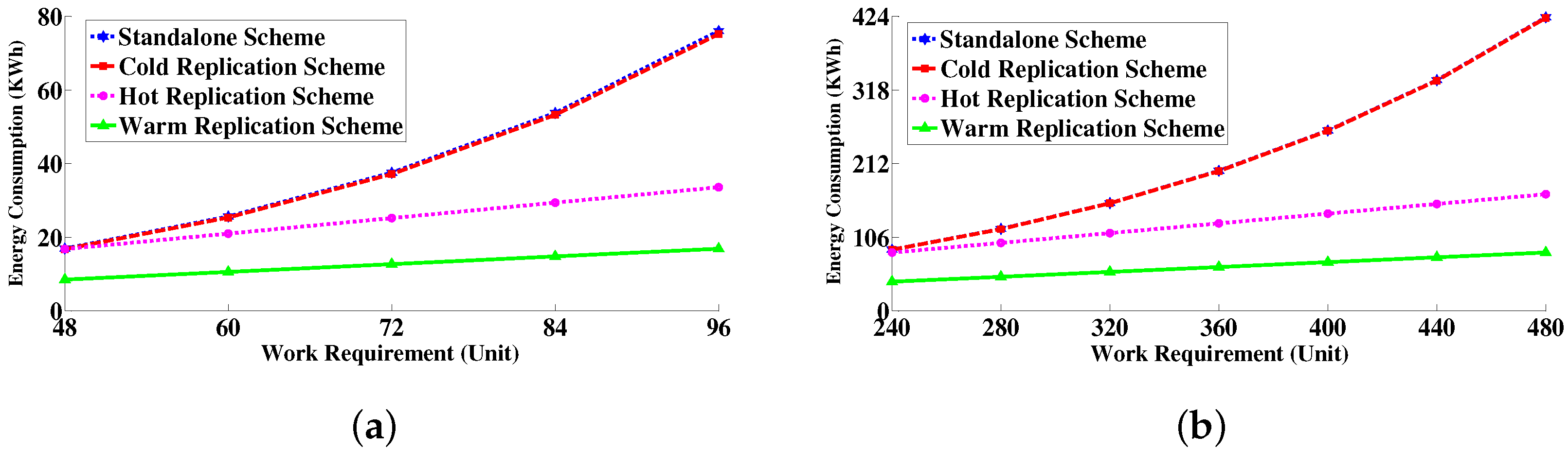
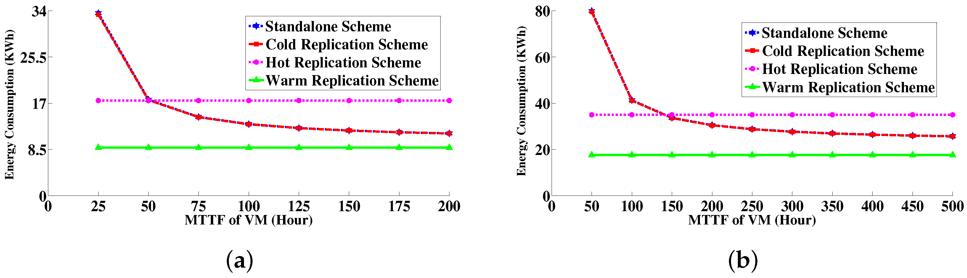
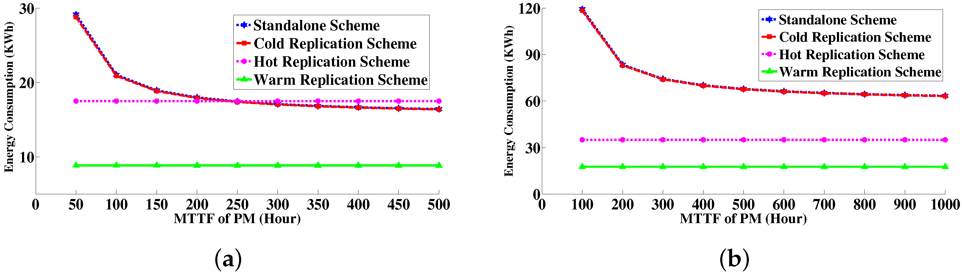
6.4.3. Energy Consumption Measurement

Figure 20 plots the energy consumption value for different work requirements especially for the work requirement below the MTTF value of VM (48 h in Set1, 240 h in Set2). We consider this measurement because the job execution is more affected by VM failure due to the higher probability/frequency of VM failure (0.8 for Set1, 0.75 for Set2) than PM failure. Note that we get the optimum energy consumption in warm replication scheme, but not in hot replication. On the other hand, energy consumption in standalone and cold replication scheme is less than in hot replication, because in hot replication scheme, we run two copies of VM independently for executing the same job and this accounts for the higher energy consumption. In addition, the difference in energy consumption between the standalone and cold replication scheme is negligible as their job completion time varies a little.

Further, we show that the energy consumption value for different work requirements is greater than the MTTF value of VM in Figure 21. Energy consumption in warm replication scheme is the least, but not in hot replication. In addition, energy consumption in the standalone and cold replication scheme increases rapidly compared to the other schemes as the work requirement increases, because the completion time correspondingly increases rapidly.

Figure 22 shows the energy consumption value with respect to MTTF of VM for work requirement $x=50$ and $x=100$ respectively as the job completion time in Figure 17. Expected energy consumption in warm replication scheme improves a bit as the MTTF increases and does not vary in hot replication though there is no interruption in execution. On the other hand, in the standalone and cold replication scheme, the energy consumption decreases gradually as MTTF increases similar to the job completion time behavior in these two schemes shown in Figure 17.

Similar to Figure 22, we show the energy consumption value with respect to MTTF of PM for work requirement $x=50$ and $x=100$ in Figure 23. Expected energy consumption in the warm replication scheme improves a bit as the MTTF increases and does not vary in hot replication though there is no interruption in execution likewise in Figure 22. On the other hand, in the standalone and cold replication scheme, the energy consumption decreases gradually as MTTF increases similarly to the job completion time behavior in these two schemes shown in Figure 18.

Thus, we can conclude that the warm replication scheme is the best choice for reducing/optimizing energy consumption, but we can employ the standalone or cold replication scheme when the work requirement is not very high, especially when it is less than the MTTF value of VM, because we need to take more steps in warm replication than in the standalone or cold replication scheme, e.g., periodic mirroring of the execution states in standby, and so on. In addition, when the work requirement is low, we can directly use the standalone scheme instead of the cold replication scheme, because in the cold replication scheme we need to keep an extra copy of the system ready, i.e, on standby, which is a wastage of resources.

7. Conclusion and Future Work

In this paper, we have developed analytical models of job execution through VM for cloud computing systems. We introduced a power consumption model which discusses the measurement of power consumption at different modes of operation and the associated energy consumption. A method to measure the energy consumption based on the structure-state process for job execution in different replication schemes has been provided. The analytical modeling approach has been validated with simulation using CloudSim. In the numerical examples, we have shown the effectiveness of replication schemes on energy consumption as well as job completion time.

In this paper, we have bounded the execution with single-task jobs. A future direction is to extend this work for jobs with different priorities and batch-tasks to make it more realistic and practical.

References

1. Ghosh, R.; Longo, F.; Naik, V.K.; Trivedi, K.S. Modeling and performance analysis of large scale iaas clouds. Future Gener. Comput. Syst. 2013, 29, 1216–1234. [Google Scholar] [CrossRef]
2. Khazaei, H.; Misic, J.; Misic, V. A Fine-Grained Performance Model of Cloud Computing Centers. IEEE Trans. Parallel Distrib. Syst. 2013, 24, 2138–2147. [Google Scholar] [CrossRef]
3. Mastroianni, C.; Meo, M.; Papuzzo, G. Probabilistic Consolidation of Virtual Machines in Self-Organizing Cloud Data Centers. IEEE Trans. Cloud Comput. 2013, 1, 215–228. [Google Scholar] [CrossRef]
4. Beloglazov, A.; Abawajy, J.; Buyya, R. Energy-aware resource allocation heuristics for efficient management of data centers for cloud computing. Future Gener. Comput. Syst. 2012, 28, 755–768. [Google Scholar] [CrossRef]
5. Mastroianni, C.; Meo, M.; Papuzzo, G. Self-economy in cloud data centers: Statistical assignment and migration of virtual machines. In Euro-Par 2011 Parallel Processing; Springer: Berlin, Germany; Heidelberg, Germany, 2011; pp. 407–418. [Google Scholar]
6. Ben-Yehuda, O.; Schuster, A.; Sharov, A.; Silberstein, M.; Iosup, A. ExPERT: Pareto-Efficient Task Replication on Grids and a Cloud. In Proceedings of the IEEE 26th International Parallel Distributed Processing Symposium (IPDPS), Shanghai, China, 21–25 May 2012; pp. 167–178.
7. Bauer, E.; Adams, R. Reliability and Availability of Cloud Computing; Wiley-IEEE Press: Hoboken, NJ, USA, 2012. [Google Scholar]
8. Lamport, L.; Shostak, R.; Pease, M. The Byzantine generals problem. ACM Trans. Program. Lang. Syst. (TOPLAS) 1982, 4, 382–401. [Google Scholar] [CrossRef]
9. Borthakur, D. The hadoop distributed file system: Architecture and design. Hadoop Proj. Website 2007, 11, 21. [Google Scholar]
10. Kulkarni, V.G.; Nicola, V.F.; Trivedi, K.S. On Modeling the Performance and Reliability of Multi-mode Computer Systems. J. Syst. Softw. 1986, 6, 175–182. [Google Scholar] [CrossRef]
11. Kulkarni, V.G.; Nicola, V.F.; Trivedi, K.S. The Completion Time of a Job on Multimode Systems. Adv. Appl. Probab. 1987, 19, 932–954. [Google Scholar] [CrossRef]
12. Machida, F.; Nicola, V.F.; Trivedi, K.S. Job completion time on a virtualized server with software rejuvenation. ACM J. Emerg. Technol. Comput. Syst. (JETC) 2014, 10, 10. [Google Scholar] [CrossRef]
13. Stedman, R. Reducing Desktop PC Power Consumption Idle and Sleep modes; Technical report; Technology Strategist, Advanced Software Technology, Dell Computer Corporation: Round Rock, TX, USA, 20 June 2005. [Google Scholar]
14. Calculating Your Energy Consumption; Technical Report 4AA2-XXXXENUC; Hewlett-Packard Development Company: Palo Alto, CA, USA, December 2008.
15. Kusic, D.; Kephart, J.O.; Hanson, J.E.; Kandasamy, N.; Jiang, G. Power and performance management of virtualized computing environments via lookahead control. Cluster Comput. 2009, 12, 1–15. [Google Scholar] [CrossRef]
16. Chen, X.; Lu, C.D.; Pattabiraman, K. Failure Analysis of Jobs in Compute Clouds: A Google Cluster Case Study. In Proceedings of the International Symposium on Software Reliability Engineering (ISSRE), Naples, Italy, 3–6 November 2014.
17. Mondal, S.K.; Machida, F.; Muppala, J.K. Service Reliability Enhancement in Cloud by Checkpointing and Replication. In Principles of Performance and Reliability Modeling and Evaluation; Springer: Berlin, Germany, 2016; pp. 425–448. [Google Scholar]
18. Di, S.; Kondo, D.; Cappello, F. Characterizing Cloud Applications on a Google Data Center. In Proceedings of the 42nd International Conference on Parallel Processing (ICPP), Lyon, France, 1–4 October 2013; pp. 468–473.
19. Mahesri, A.; Vardhan, V. Power consumption breakdown on a modern laptop. In Power-Aware Computer Systems; Springer: Berlin, Germany, 2005; pp. 165–180. [Google Scholar]
20. Huang, S.; Huang, J.; Dai, J.; Xie, T.; Huang, B. The HiBench benchmark suite: Characterization of the MapReduce-based data analysis. In Proceedings of the 26th International Conference on IEEE Data Engineering Workshops (ICDEW), Long Beach, CA, USA, 1–6 March 2010; pp. 41–51.
21. Benchmarking Hadoop & HBase on Violin; Technical report; Big Data-Violin Memory: Santa Clara, CA, USA, 2013.
22. Calheiros, R.; Ranjan, R.; De Rose, C.; Buyya, R. Cloudsim: A novel framework for modeling and simulation of cloud computing infrastructures and services. Technical Report, GRIDS-TR-2009-1; Grid Computing and Distributed Systems Laboratory, The University of Melbourne: Melbourne, Australia, March 2009. [Google Scholar]
23. Calheiros, R.; Ranjan, R.; Beloglazov, A.; De Rose, C.; Buyya, R. CloudSim: A toolkit for modeling and simulation of cloud computing environments and evaluation of resource provisioning algorithms. Softw. Pract. Exp. 2011, 41, 23–50. [Google Scholar] [CrossRef]
24. Mondal, S.K.; Muppala, J.K. Energy Modeling of Different Virtual Machine Replication Schemes in a Cloud Data Center. In Proceedings of the Internet of Things (iThings), 2014 IEEE International Conference on, and Green Computing and Communications (GreenCom), IEEE and Cyber, Physical and Social Computing (CPSCom), Taipei, Taiwan, 1–3 September 2014; pp. 486–493.
25. Mondal, S.K.; Muppala, J.K.; Machida, F.; Trivedi, K.S. Computing Defects per Million in Cloud Caused by Virtual Machine Failures with Replication. In Proceedings of the 2014 IEEE 20th Pacific Rim International Symposium on IEEE Dependable Computing (PRDC), Singapore, 19–21 November 2014; pp. 161–168.
26. Mondal, S.; Yin, X.; Muppala, J.; Alonso Lopez, J.; Trivedi, K. Defects per Million Computation in Service-Oriented Environments. IEEE Trans. Serv. Comput. 2015, 8, 32–46. [Google Scholar] [CrossRef]
27. Hines, M.R.; Gopalan, K. Post-copy based live virtual machine migration using adaptive pre-paging and dynamic self-ballooning. In Proceedings of the 2009 ACM SIGPLAN/SIGOPS International Conference on Virtual Execution Environments, Washington, DC, USA, March 2009; pp. 51–60.
28. Virtual Machine Migration Comparison: VMWare VSphere vs. Microsoft Hyper-V. Test Report; Principled Technologies Inc.: Durham, NC, USA, October 2011.
Figure 1. Continuous time Markov chain (CTMC) model for system with standalone scheme.
Electronics 05 00037 g001
Figure 2. CTMC model for system with cold replication.
Electronics 05 00037 g002
Figure 3. Approximated continuous time Markov chain (CTMC) model for system with cold replication.
Electronics 05 00037 g003
Figure 4. CTMC model for system with warm replication.
Electronics 05 00037 g004
Figure 5. Approximated CTMC model for system with warm replication.
Electronics 05 00037 g005
Figure 6. CTMC model for system with hot replication.
Electronics 05 00037 g006
Figure 7. Approximated CTMC model for system with hot replication.
Electronics 05 00037 g007
Figure 8. Comparison of mean job completion time between simulative solution and analytic modeling solution in standalone scheme for different work requirements. (a) For Set1 parameter values; (b) For Set2 parameter values.
Electronics 05 00037 g008
Figure 9. Comparison of mean job completion time between simulative solution and analytic modeling solution in cold replication for different work requirements. (a) For Set1 parameter values; (b) For Set2 parameter values.
Electronics 05 00037 g009
Figure 10. Comparison of mean job completion time between simulative solution and analytic modeling solution in warm replication for different work requirements. (a) For Set1 parameter values; (b) For Set2 parameter values.
Electronics 05 00037 g010
Figure 11. Mean job completion time and its standard deviation (STD) obtained from simulation. (a) Standalone scheme; (b) Cold replication scheme; (c) Warm replication scheme.
Electronics 05 00037 g011
Figure 12. Comparison of expected energy consumption between simulative solution and analytic modeling solution in standalone scheme for different work requirements. (a) For Set1 parameter values; (b) For Set2 parameter values.
Electronics 05 00037 g012
Figure 13. Comparison of expected energy consumption between simulative solution and analytic modeling solution in cold replication for different work requirements. (a) For Set1 parameter values; (b) For Set2 parameter values.
Electronics 05 00037 g013
Figure 14. Comparison of expected energy consumption between simulative solution and analytic modeling solution in warm replication for different work requirements. (a) For Set1 parameter values; (b) For Set2 parameter values.
Electronics 05 00037 g014
Figure 15. Mean job completion time for different work requirements. (a) For Set1 parameter values; (b) For Set2 parameter values.
Electronics 05 00037 g015
Figure 16. Mean time to recovery in different replication schemes. (a) For Set1 parameter values; (b) For Set2 parameter values.
Electronics 05 00037 g016
Figure 17. Mean job completion time by varying the mean time to failure (MTTF) of virtual machine (VM). (a) x = 50 unit (Set1); (b) x = 100 unit (Set1).
Electronics 05 00037 g017
Figure 18. Mean job completion time by varying the MTTF of physical machine (PM). (a) x = 50 unit (Set1); (b) x = 100 unit (Set1).
Electronics 05 00037 g018
Figure 19. Cumulative distribution function (CDF) of job completion time. (a) For Set1 parameter values ( x = 50 unit); (b) For Set2 parameter values ( x = 300 unit).
Electronics 05 00037 g019
Figure 20. Expected energy consumption for different work requirements. (a) x 1 / γ v m (Set1); (b) x 1 / γ v m (Set2).
Electronics 05 00037 g020
Figure 21. Expected energy consumption for different work requirements. (a) x 1 / γ v m (Set1); (b) x 1 / γ v m (Set2).
Electronics 05 00037 g021
Figure 22. Expected energy consumption with respect to MTTF of VM. (a) x = 50 unit (Set1); (b) x = 100 unit (Set1).
Electronics 05 00037 g022
Figure 23. Expected energy consumption with respect to MTTF of PM. (a) x = 50 unit (Set1); (b) x = 100 unit (Set1).
Electronics 05 00037 g023