Article

A Raspberry Pi Cluster Instrumented for Fine-Grained Power Measurement †

Electrical and Computer Engineering, University of Maine, Orono, ME 04469, USA
*
Author to whom correspondence should be addressed.
This paper is an extended version of our paper published in 2014 First International Workshop on Hardware-Software Co-Design for High Performance Computing, New Orleans, LA, USA, 16–21 November 2014.
Electronics 2016, 5(4), 61; https://doi.org/10.3390/electronics5040061
Submission received: 30 April 2016 / Revised: 9 September 2016 / Accepted: 13 September 2016 / Published: 23 September 2016
(This article belongs to the Special Issue Raspberry Pi Technology)

Abstract

:
Power consumption has become an increasingly important metric when building large supercomputing clusters. One way to reduce power usage in large clusters is to use low-power embedded processors rather than the more typical high-end server CPUs (central processing units). We investigate various power-related metrics for seventeen different embedded ARM development boards in order to judge the appropriateness of using them in a computing cluster. We then build a custom cluster out of Raspberry Pi boards, which is specially designed for per-node detailed power measurement. In addition to serving as an embedded cluster testbed, our cluster’s power measurement, visualization and thermal features make it an excellent low-cost platform for education and experimentation.

1. Introduction

Embedded systems and modern supercomputers, while at opposite ends of the computing spectrum, share an important design constraint: the need to have the highest possible performance while staying inside of a power budget. As the number of cores in large computers increases, the per-core power usage becomes increasingly important.
One way to address this power consumption problem is to replace high-end server central processing units (CPUs) with the low power processors more traditionally found in embedded systems. The use of embedded processors in supercomputers is not new; the various BlueGene [1,2,3] machines use embedded-derived PowerPC chips. The ARM embedded architecture has drastically increased in performance, including the introduction of 64-bit processors for use in high-end cell phones. This has led to a new source of well-supported, inexpensive, relatively high-performing embedded processors ready for use in supercomputing and cluster applications.
Despite the seeming inevitability of large ARM supercomputers, the actual uptake has been extremely slow. As of November 2015, there are still no ARM-based systems on the Top500 supercomputer list [4].
In order to evaluate the future potential of large ARM-based systems we have built a computing cluster out of commodity ARM development boards. We first evaluate seventeen different ARM-based systems with the goal of finding a low-cost, low-power, high-performance board suitable for cluster use. By using existing boards, we reduce development time and cost, at the expense of possibly missing out on some features that are key to large-scale cluster development (most notably, graphics processing unit (GPU) acceleration, fast memory hierarchies and high-speed network interconnects).
After weighing the various tradeoffs, we chose the Raspberry Pi as the basis for our cluster. Our current cluster is made out of 25 Raspberry Pi Model 2B systems linked together with 100 MB Ethernet. It can obtain 15.4 billion floating point operations per second (GFLOPS) of performance, while consuming 93 W. While these results are not remarkable compared to a high-end Intel x86 server, we have included some features in our cluster that make it an interesting measurement and educational tool. We have per-node visualization via 8×8 light-emitting diode (LED) displays that allow the detailed machine state to be seen at a glance. We also have detailed, per-node power measurement capabilities, which allow fine granularity measurements of cluster power consumption. We primarily use this cluster as an educational tool to provide low-cost hands-on experience in a cluster computing class.

2. Experimental Section

2.1. Board Comparison

Before designing our cluster, we evaluated the power and performance tradeoffs found in seventeen different commodity 32-bit and 64-bit ARM boards, as listed in Table 1. The boards, all running Linux, span a wide variety of speeds, cost and processor types. More complete info on the hardware capabilities of the boards can be found in Appendix A.

2.1.1. Experimental Setup

During the experiments we configure the machines as if they were a node in a larger cluster. No extraneous devices (keyboards, mice, monitors, external drives) are attached during testing; the only connections are the power supplies and network cables (with the exception of the Chromebook, which has a wireless network connection and a laptop screen). Machines that did not have native Ethernet were provided with a USB Ethernet adapter.

2.1.2. Benchmarking Programs

Choosing a representative set of High Performance Computing (HPC) benchmarks remains difficult, as cluster performance is tightly tied to the underlying workload. We chose two HPC benchmarks that are widely used in cluster benchmarking: Linpack and STREAM.
High-performance Linpack (HPL) [5] is a portable version of the Linpack linear algebra benchmark for distributed-memory computers. It is commonly used to measure the performance of supercomputers worldwide, including the twice-a-year Top500 Supercomputer list [4]. The program tests the performance of a machine by solving complex linear systems through use of basic linear algebra subprograms (BLAS) and the message-passing interface (MPI).
For our experiments, mpich2 [6] was installed on each machine to provide a message passing interface (MPI), and the OpenBLAS [7] library was installed on each machine to serve as the BLAS.
The second benchmark we use is STREAM [8], which tests a machine’s memory performance. STREAM performs operations, such as copying bytes in memory, adding values together and scaling values by another number. STREAM completes these operations and reports the time it took, as well as the speed of the operations.
We compiled our benchmarks with the version of gcc that was installed on the various machines (typically it was gcc 4.9, as most machines were running the Raspbian Jessie Linux distribution). We used the default compiler options when compiling.
We did not use any digital signal processing (DSP) or graphics programming unit (GPU) acceleration, even though many of the boards support this. In general, the boards do not support Open Computing Language (OpenCL) or any other abstraction layer on top of the accelerators. To gain access to the DSP or GPU would require extensive custom coding for each individual board, and often, these interfaces are not well documented. The Jetson TX-1 board does support NVIDIA CUDA, so we tried running HPL_cuda on the board. This consistently crashed the system, so we were unable to obtain results. The TX-1 GPU is optimized for single-precision floating point, so direct comparisons against the CPU results (which use double-precision) would not be possible.

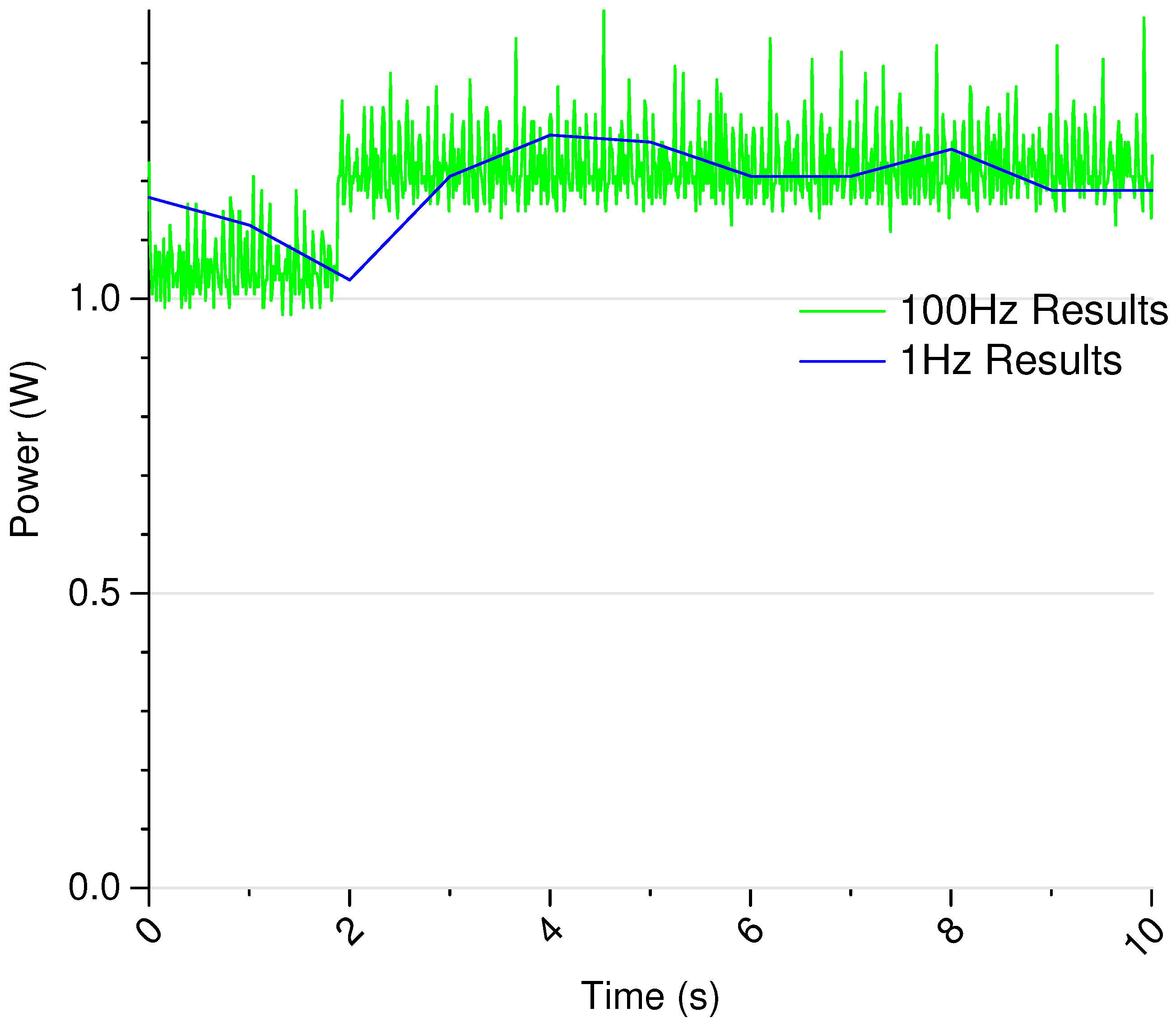
2.1.3. Power Measurement

The power consumed by each machine was measured and logged using a WattsUpPro [9] power meter. The meter was configured to log the power at its maximum sampling speed of once per second.
The power readings were gathered on a separate machine from the one running the benchmarks. For proper analysis, the timestamps of the power readings need to match up with the start and stop times of the benchmarks. We did this by synchronizing the clocks of the two machines to the same network time protocol (NTP) time server before starting the runs. There is some potential for drift, but since our power meter only provides one second of resolution, this solution was deemed to be good enough.

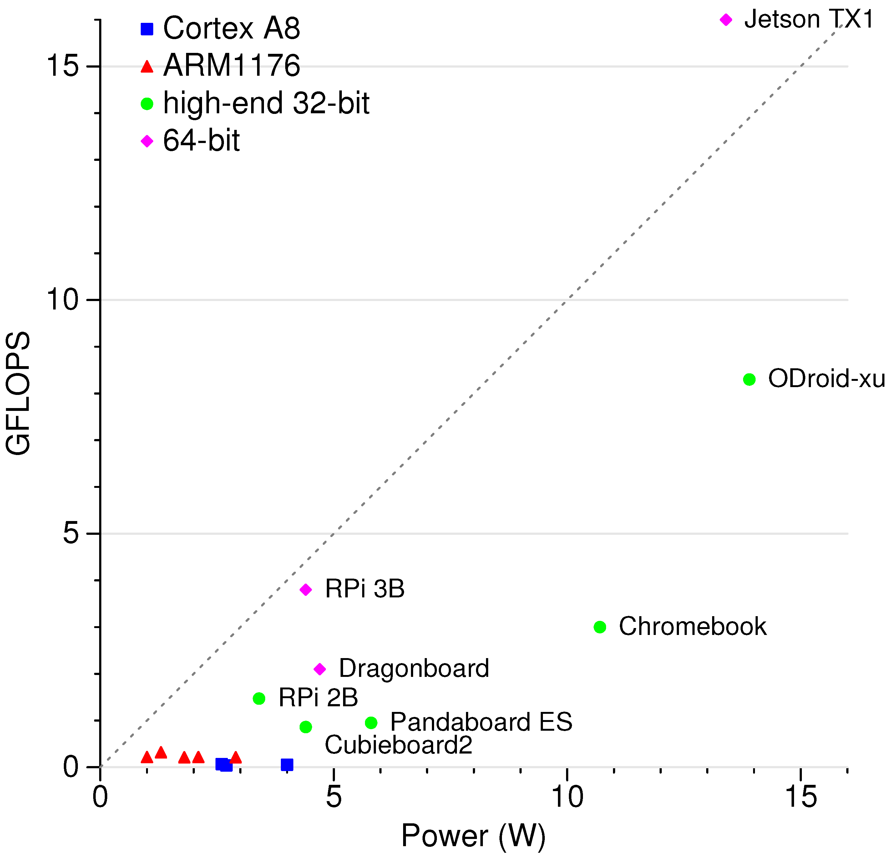
2.1.4. HPL FLOPS Results

Table 2 summarizes the floating point operations per second (FLOPS) results when running HPL. We took many results for each board, varying the N term to find the maximum performance. N is the problem size: usually higher is better, but at some point, performance starts declining as the amount of memory available is exhausted.
The FLOPS value is unexpectedly low on the Cortex-A8 machines; the much less advanced ARM1176 Raspberry-Pi obtains better results. This is most likely due to the “VFP-lite” floating point unit found in the Cortex-A8, which takes 10 cycles per operation rather than just one. It may be possible to improve these results by changing the gcc compiler options; by default, strict IEEE-FP correctness is chosen over raw speed.
The ARM1176-based systems (low-end Raspberry Pis) all cluster together with similar performance, differing mostly by the CPU clock frequency.
The more advanced Cortex-A9 and Cortex-A7 systems have a noticeable improvement in floating point performance. This includes the Pandaboard, Cubieboard2 and Raspberry Pi Model 2B. Some of this is due to these machines having multiple cores. We do not have numbers for the Trimslice: building a BLAS for it proved difficult, as it lacks NEON support (NEON is optional on Cortex-A9), and a later hardware failure prevented further testing.
The Cortex-A15 machines (Chromebook and Odroid-xU) have an even greater boost in FLOPS, with the highest performance of the 32-bit systems.
The 64-bit systems have high performance, as well, with the high-end Cortex-A57 (Jetson TX-1) with the best performance and the lower end Cortex-A53 systems (Dragonboard, Raspberry Pi Model 3B) not far behind.
The Raspberry Pi Model 3B posed some interesting challenges. Unlike previous models, when running HPL, the chip can overheat and produce wrong results or even crash [10]. With an adequate heat sink, cooling and boot loader over-volt settings, an impressive 6.4 GFLOPS can be obtained, but on stock systems, the CPU overheats and/or clocks down the CPU, with much lower results are obtained.
For comparison, we show results from a few x86 machines. We find that while the high-end ARM systems can outperform a low-end atom-based x86 server, recent high-end AMD and Intel servers have at least an order of magnitude more FLOPS than any of the ARM systems.

2.1.5. HPL FLOPS per Watt Results

Table 2 also shows the GFLOPS per average power results (GFLOPS/W). This is shown graphically in Figure 1, where an ideal system optimizing both metrics would have points in the upper left. In this metric, the 64-bit machines perform best by a large margin. The Jetson TX-1 (and properly-cooled Raspberry Pi 3B) break the 1 GFLOP/W barrier. The Chromebook is at a disadvantage compared to the other boards, as it is a laptop and has a display that was operating while the test was running. This is most noticeable in the idle power being higher than all of the other boards.
While the 64-bit machines have much better efficiency than earlier processors, a high-end x86 server can still obtain twice the power per watt than even the best ARM system to which we have access.

2.1.6. HPL FLOPS per Cost Results

Table 2 also shows the FLOPS per dollar cost (purchase price) of the system (higher is better); this is also shown in Figure 2, where an ideal system optimizing both would have points in the upper left. The Raspberry Pi 3 performs impressively on the MFLOPS/US$ metric, matching a high-end x86 server. The Raspberry Pi Zero is a surprise contender, due mostly to its extremely low cost.

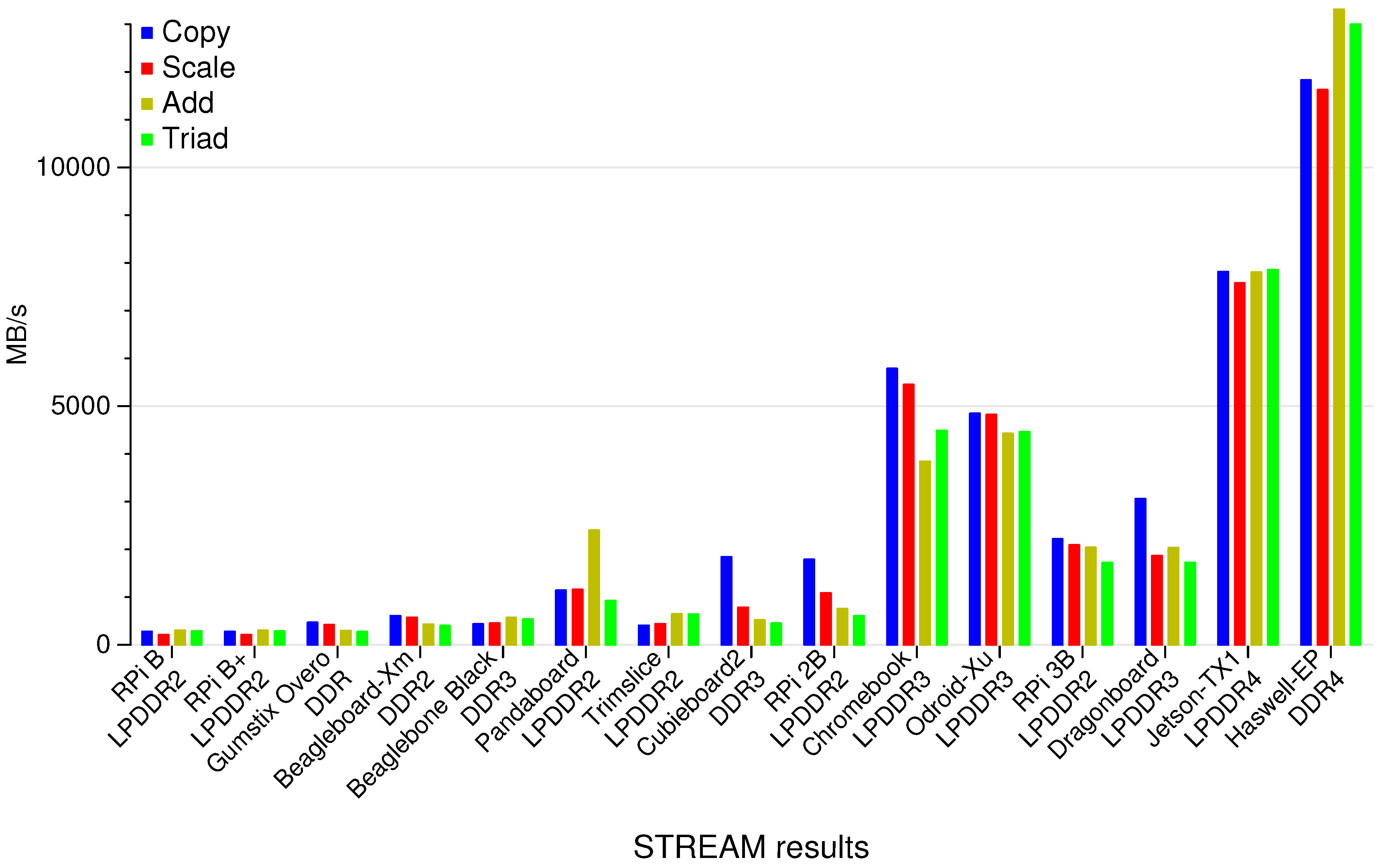
2.1.7. STREAM Results

We ran Version 5.10 of the STREAM benchmark on all of the machines. We use the default array size of 10 million (except for the Gumstix Overo, which only has 256 MB of RAM, so a problem size of 9 million was used). Figure 3 shows a graph of the performance of each benchmark. The more advanced Cortex-A15 chips have much better memory performance than the earlier boards, most likely due to the use of dual-channel low-power double-data rate (LPDDR3) memory. The Jetson-TX1 has extremely high memory performance, although not quite as high as a full x86 server system.
To fully understand the results, some knowledge of modern memory infrastructure is needed. On desktop and server machines, synchronous dynamic random access memory (SDRAM) is used, and the interface has been gradually improving over the years from DDR (double data rate) to DDR2, DDR3 and now DDR4. Each new generation improves the bandwidth by increasing how much data can be sent per clock cycle, as well as by increasing the frequency. Power consumption is also important, and the newer generations reduce the bus voltage to save energy (2.5 V in DDR, 1.8 V in DDR2, 1.5 V in DDR3 and down to 1.2 V in DDR4). Embedded systems can use standard memory, but often they use mobile embedded SDRAM (low-power), such as LPDDR2, LPDDR3 or LPDDR4. This memory is designed with embedded systems in mind, so often trade off performance for lower voltages, extra sleep states and other features that allow using less power.
One factor affecting performance is the number of DRAM (dynamic random access memory) channels the device has: despite having similar CPUs, the Trimslice only has a single channel to memory, while the Pandaboard has two, and the memory performance is correspondingly better.
The bus frequency can also make a difference. Note that the Odroid-xU and the Dragonboard both have LPDDR3 memory; however, the Odroid runs the memory bus at 800 MHz versus the Dragonboard’s 533 MHz, and the STREAM results for Odroid are correspondingly better.

2.1.8. Summary

Results of both the HPL and STREAM benchmarks show the Jetson TX1 machine as the clear winner on performance, STREAM and performance per Watt metrics. If cost is factored in, the Raspberry Pi 3B makes a strong case, although it has the aforementioned problems with overheating.
The Pi 3B and Jetson TX-1 were not yet released when we started building our cluster, so our design choice was made without those as options. At the time, the best performing options other than the Pi were the Chromebook (which has a laptop form factor and no wired Ethernet) and the Odroid-xU (which was hard to purchase through our university’s procurement system). We chose to use Raspberry Pi B boards for various practical reasons. A primary one was cost and the ease of ordering large numbers at once. Another important concern is the long-term availability of operating support and updates; the Raspberry Pi foundation has a much stronger history of this than the manufacturers of other embedded boards.
Our cluster originally used Model B boards, and we have since updated to B+ and then 2B. The compatible design of the Raspberry Pi form factor means it should be easy to further upgrade the system to use the newer and better performing Model 3B boards.

2.2. Cluster Design

Based on the analysis in Section 2.1, we chose Raspberry Pi Model 2B boards as the basis of our cluster. The Raspberry Pi boards provide many positive features, including small size, low cost, low power consumption, a well-supported operating system and easy access to general-purpose input/output (GPIO) pins for external devices. Figure 4 shows the cluster in action. The compute part of the cluster (compute nodes plus network switch) costs roughly US$2200; power measurement adds roughly $200; and the visualization display costs an additional $700.

2.2.1. Node Installation and Software

Each node in the cluster consists of a Raspberry Pi Model 2B with its own 4 GB SD card. Each node has an installation of the Raspbian operating system, which is based on Debian Linux and designed specifically for the Raspberry Pi.
One node is designated as the head node and acts as a job submission server, central file server and network gateway. The file system is shared via Network File System (NFS) and subsequently mounted by the sub-nodes. Using NFS allows programs, packages and features to be installed on a single file system and then shared throughout the network, which is faster and easier to maintain than manually copying files and programs around. Passwordless SSH (Secure Shell) allows easily running commands on the sub-nodes. MPI (message passing interface) is installed to allow cluster-wide parallel jobs. The MPI implementation used for this cluster is MPICH2, a free MPI distribution written for UNIX-like operating systems. For job submission, the Slurm [11] batch scheduler is used.
The nodes are connected by 100 MB Ethernet, consisting of a 48-port 10/100 network switch, which draws approximately 20 Watts of power.

2.2.2. Node Arrangement and Construction

The initial cluster has 24 compute nodes plus one head node. It is designed so expansion to 48 nodes is possible.
A Corsair CX430 ATX power supply powers the cluster. The Pi boards are powered by the supply’s 5-V lines, as well as via the 12-V lines through a direct current (DC-DC) converter that reduces this to 5-V. We found it necessary to draw power from both the 5-V and 12-V lines of the power supply, otherwise the voltages provided would become unstable. This is typical behavior of most desktop power supplies, as they are designed to provide a minimum load on the 12-V lines, and if this load is not present, the output voltages can drift outside of specifications.
The head node is powered by the supply’s standby voltage, which allows the node to be powered up even when the rest of the cluster is off. The head node can power on and off the rest of the cluster by toggling the ATX power enable line via GPIO.
Power can be supplied to a Raspberry Pi in two ways, through the micro USB connector or through the GPIO header. The power pins on the GPIO header connect directly to the main power planes and have no protection circuitry. We use the micro USB power connector to take advantage of the fuses and smoothing capacitors that add an extra layer of protection. This did complicate construction, as we had to crimp custom micro-USB power cords to connect the Pis to the power measurement and distribution boards.
The boards are attached via aluminum standoffs in stacks of four and are placed in a large server case that has had wooden shelving added.

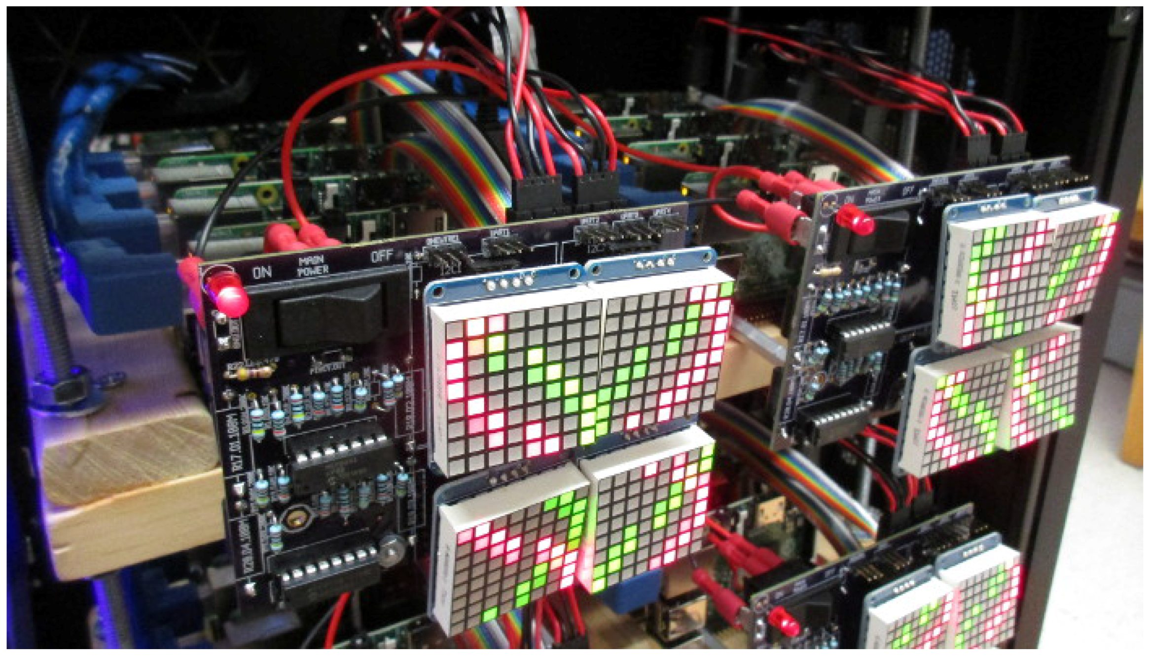
2.2.3. Visualization Displays

Two main external displays are used to visualize the cluster activity.
The first is a series of 1.2 inch bi-color 8×8 LED matrix displays (Adafruit, New York, NY, USA) attached to each node’s GPIO ribbon cable. These LED displays can be individually programmed via the nodes’ i2c interface. These per-node displays can be controlled in parallel via MPI programs. This not only allows interesting visualization and per-node system information, but provides the possibility for students to experience plainly visible representations of their underlying MPI programs.
The second piece of the front end is an LCD-PI32 3.2 inch LCD touchscreen (Adafruit, New York, NY, USA) that is programmed and controlled using the head node’s SPI interface. This screen allows a user to view overall power and performance information, as well as check the status of jobs running on all nodes of the cluster.

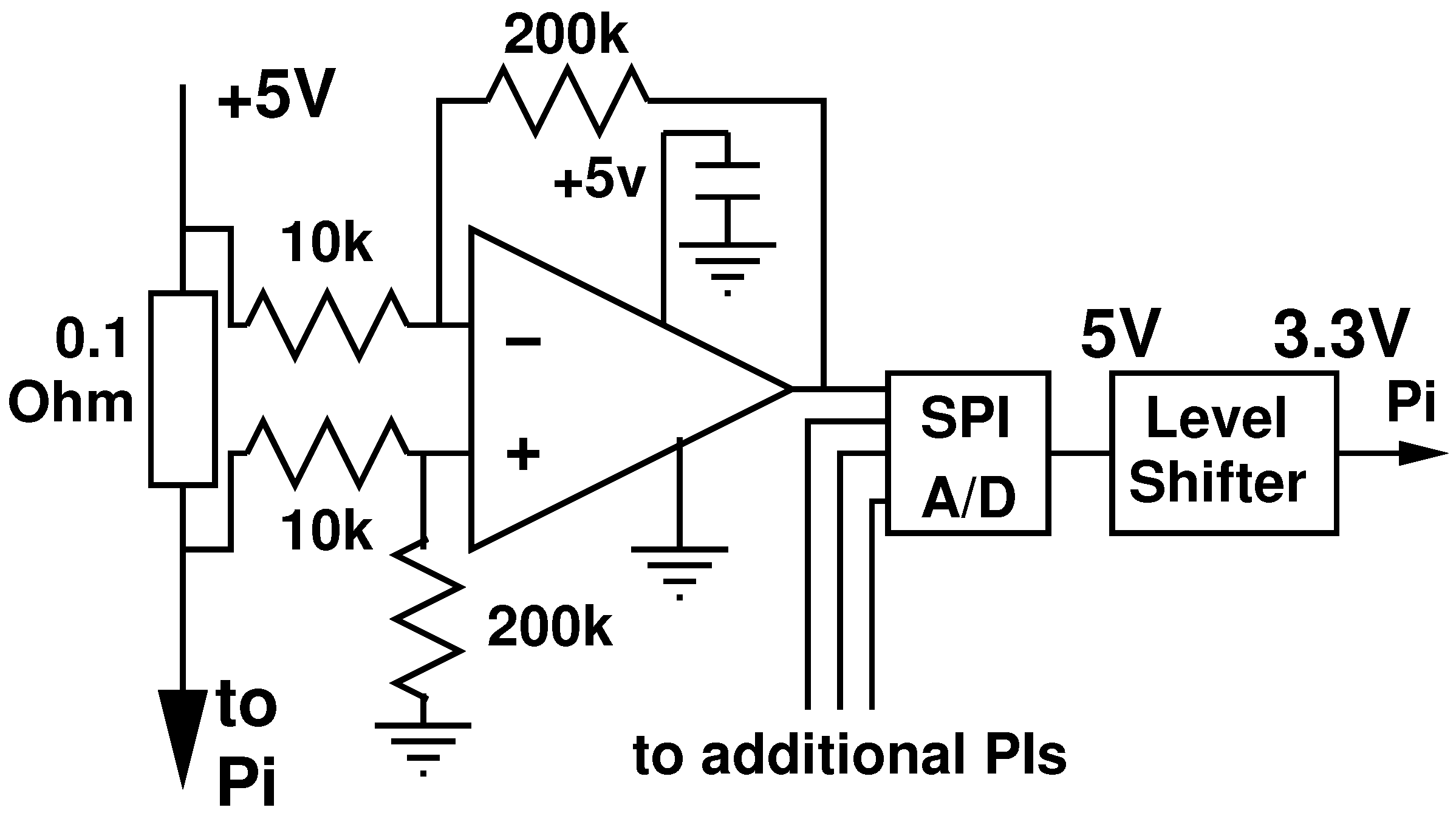
2.2.4. Power Measurement

Each node has detailed power measurement provided by a circuit as shown in Figure 5. The current consumed is calculated from the voltage drop across a 0.1-Ohm sense resistor, which is amplified by 20 with an MCP6044 op-amp and then measured with an MCP3008 SPI A/D converter. Multiplying overall voltage by the calculated current gives the instantaneous power being consumed. There is one power measurement board for each group of four nodes; the first node in each group is responsible for reading the power via the SPI interface.
An example power measurement for the full cluster is shown in Figure 6. The workload is a 10 k 12-node HPL run with 5 s of sleep on either side. While sampling frequencies up to at least 1 kHz are possible, in this run, the power is sampled at 4 Hz in order to not clutter up the graph.
One of the nodes (node052) is currently down, and the power measurement of three of the nodes (node030, node033 and node010) is currently malfunctioning. The rest of the nodes are measuring fine, and you can see detailed behavior across the cluster. Half of the nodes are idle, and the rest show periodic matching peaks and troughs as the workload calculates and then transmits results.
One advantage of our custom power measurement circuits is that we can sample at a high granularity. We can alternately measure system-wide power with a WattsUpPro [9] power meter. The WattsUpPro can only sample power at 1-Hz resolution, which can miss fine-grained behaviors. Figure 7 shows the loss of detail found if the sampling frequency is limited to 1-Hz.

2.2.5. Temperature Measurement

In addition to power usage, it is often useful to track per-node temperature. The Raspberry Pi has an on-chip thermometer that can be used to gather per-board temperature readings. Our power measurement boards also support the later addition of 1-wire protocol temperature probes if additional sensors are needed.

3. Results

We ran the HPL benchmark on our 25-node Raspberry Pi 2B cluster while measuring the power consumption. For comparison, we show earlier results with our prototype 32-node Pi B+ cluster (both stock, as well as overclocked to 1 GHz).

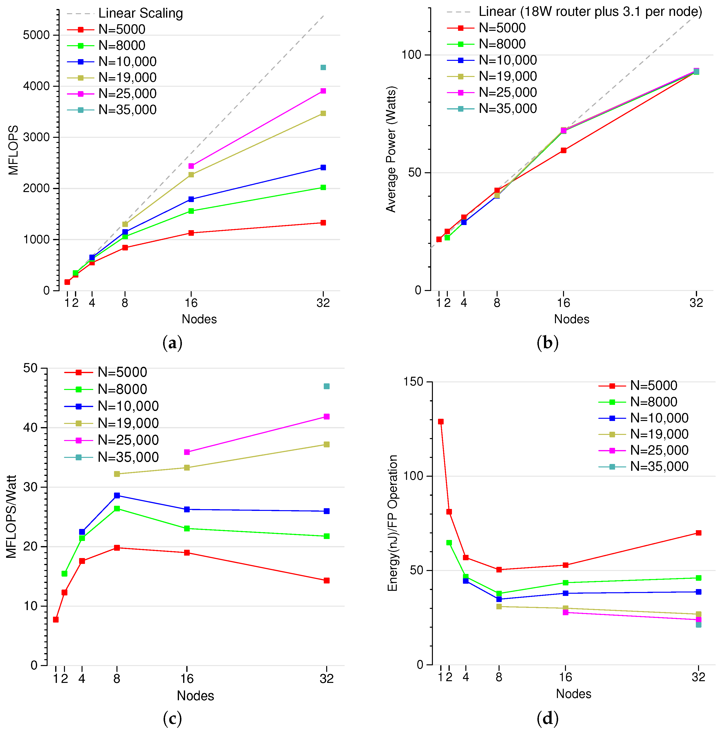
3.1. Peak FLOPS Results

Table 3 shows the peak performance of our Raspberry Pi Model 2B cluster running with 24 nodes. We find a peak of 15.5 GFLOPS while using 93.1 W for a GFLOPS/W rating of 0.166. This is much better than the results found with our prototype Raspberry Pi Model B+ cluster, even when overclocked. For comparison, we show a few Intel x86 servers; our cluster still lags those both in performance and FLOPS/W. Part of this inefficiency is due to the 20-W overhead of the network switch, which is amortized as more nodes are added.
Our cluster would have been Number 7 on the first Top500 list from June 1993 [12].

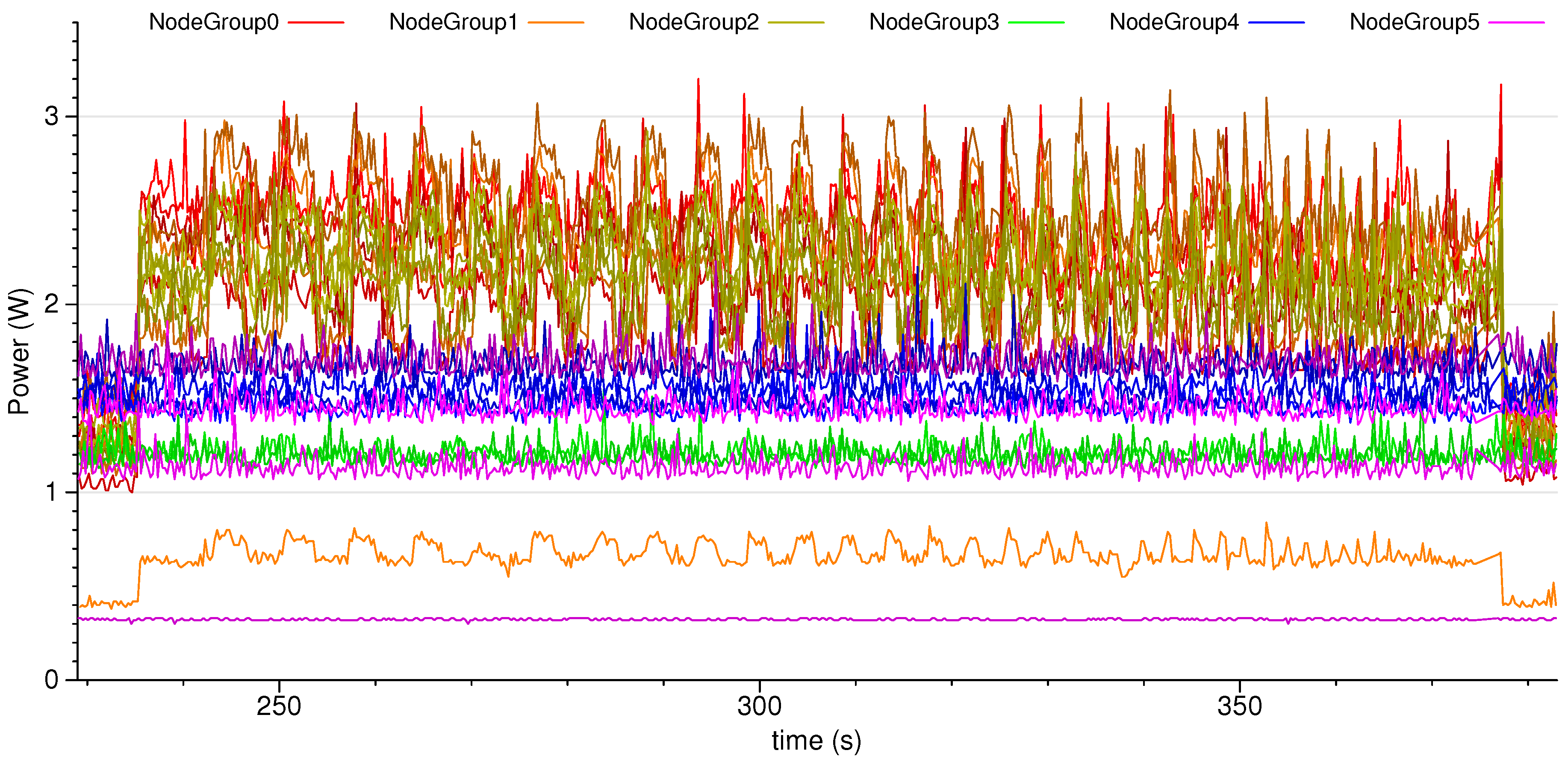
3.2. Cluster Scaling

Figure 8a shows the performance results of our prototype Model B cluster scaling as more nodes are added. Scaling behavior will be similar with our Model 2B cluster. Adding nodes continues to increase performance in an almost linear fashion, this gives hope that we can continue to improve performance by adding more nodes to the cluster.
Figure 8b shows the average power increase as nodes are added. This scales linearly, roughly proportional to 18 W (for the router) with 3.1 W for each additional node. The increase when moving from 16 to 32 nodes is less; that is because those additional nodes are Model B+ boards, which draw less power.
Figure 8c shows the performance per Watt numbers scaling as more nodes are added. This value is still increasing as nodes are added, but at a much lower level than pure performance. This is expected, as all of the boards have the same core MFLOPS/W value, so adding more is simply mitigating the static overhead power rather than making the cluster more efficient.
Figure 8d shows how many Joules of energy are used on average for each floating point operation. The optimum for a number of problem sizes is with an eight-node cluster, but the value does get lower as more nodes are added.

3.3. Summary

We find that it is possible to build a low-cost, power-instrumented, Raspberry Pi cluster that is capable of over 15 GFLOPS of performance. Due to the modular design of the Raspberry Pi boards, it should be easy to upgrade this to the newer Model 3B designs, which have GFLOPS/W results approaching those of high-end x86 servers. Despite the poor networking hardware in the Pis, we find that cluster performance keeps increasing even up to the 32 node mark. Our cluster serves as an excellent educational tool for general parallel programming, as well as for conducting detailed ARM power/performance code optimization.

4. Discussion

4.1. Related Work

We perform a price, performance and cost comparison of a large number of ARM boards. We use those results to guide the design of a cluster with per-node power instrumentation and visualization. We break the related work out by topic, as previous papers have investigated various subsets of these topics.

4.1.1. Cluster Power Measurement

Other work has been done on gathering fine-grained cluster power measurement; usually, the cluster in question runs x86 processors. Powerpack [13] is one such instrumented x86 cluster. The PowerMon2 [14] project describes small boards that can be used to instrument a large x86 cluster. Hackenberg et al. [15] describe various power measurement techniques (including Intel running average power limit (RAPL) power estimates), but again, primarily looking at x86 devices.

4.1.2. ARM HPC Performance Comparisons

Dongarra and Luszczek [16] were one of the first groups attempting to optimize for HPC performance on small boards; they created an iPad2 (Cortex A9) Linpack app showing that performance was on par with early Cray supercomputers.
Aroca et al. [17] compare Pandaboard, Beagleboard and various x86 boards with FLOPS and FLOPS/W. Their Pandaboard and Beagleboard performance numbers are much lower than the ones we measure. Jarus et al. [18] compare the power and energy efficiency of Cortex-A8 systems with x86 systems. Blem et al. [19] compare Pandaboard, Beagleboard and x86. Stanley-Marbell and Cabezas [20] compare Beagleboard, PowerPC and x86 low-power systems for thermal and power. Pinto et al. [21] compare Atom x86 vs. Cortex A9. Padoin et al. [22,23,24] compare various Cortex A8 and Cortex A9 boards. Pleiter and Richter [25] compare Pandaboard vs. Tegra2. Laurenzano et al. [26] compare Cortex A9, Cortex A15 and Intel Sandybridge and measure power and performance on a wide variety of HPC benchmarks.
Our ARM comparisons are different from the previously-mentioned work primarily by how many different boards (seventeen) that we investigated.

4.1.3. ARM Cluster Building

There are many documented cases of compute clusters built from commodity 32-bit ARM boards. Many are just brief descriptions found online; we concentrate on those that include writeups with power and HPL performance numbers.
Geveler et al. [27] build a 60-node Tegra-K1 cluster capable of being powered by solar panels. The cluster has a theoretical peak performance of 21 TFLOPS while consuming 2 kW of power, which is an efficiency of 10.5 GFLOPS/W.
Rajovic et al. [28,29] describe creating the Tibidabo cluster out of 128 Tegra 2 boards. They obtain 97 GFLOPS when running HPL on 96 nodes. Göddecke et al. [30] use this cluster on a wide variety of scientific applications and find that the energy use compares favorably with an x86 cluster.
Sukaridhoto et al. [31] create a cluster out of 16 Pandaboard-ES boards. They run STREAM and HPL on it, but do not take power measurements. Their STREAM results are much lower than ours, but the HPL FLOPS values are close.
Balakrishnan [32] investigates a six-node Pandaboard cluster, as well as a two-node Raspberry Pi cluster. He uses a WattsUpPro as we do, but only runs HPL on the Pandaboard. He finds lower results than we do with STREAM, but his HPL results on Pandaboard are much higher than ours.
Ou et al. [33] create a four-board Pandaboard cluster and measure the energy and cost efficiency of web workloads on ARM compared to x86 servers.
Fürlinger et al. [34] build a cluster out of four Apple TV devices with Cortex A8 processors. They find 16 MFlop/W. Their single-node HPL measurements are close to ours.

4.1.4. Raspberry Pi Clusters

Various groups have built Raspberry Pi clusters, we focus here on ones that were reported with HPL as a benchmark or else have large numbers of nodes. None of them are instrumented for per-node power measurements like ours is. Pfalzgraf and Driscoll [35] create a 25-node Raspberry Pi cluster, but do not provide power or FLOPS results. Kiepert [36] builds a 32-node Raspberry Pi cluster. He includes total power usage of the cluster, but does not include floating point performance results. Tso et al. [37] build a 56-node Raspberry Pi “cloud” cluster. Cox et al. [38] construct a 64-node Raspberry Pi cluster. They obtain a peak performance of 1.14 GFLOPS, which is much less than we find with 32 nodes on our cluster. Abrahamsson et al. [39] built a 300-node Raspberry Pi cluster.

4.1.5. Summary

There is much existing related work; our work is different primarily in the number of boards investigated and in the per-node power measurement capabilities of the finished cluster.
One worrying trend found in the related works is the wide variation in performance measurements. For the various ARM boards, the STREAM and HPL FLOPS results should be consistent, yet the various studies give widely varying results for identical hardware.
Differences in HPL results are most likely due to different BLAS libraries being used, as well as the difficulty finding a “peak” HPL.datfile that gives the best performance.
It is unclear why STREAM results differ so widely, as there are fewer variables involved. It could be due to differences in compiler, compiler options or problem size, but most papers do not give details on how the benchmarks were built, nor are the compiled binaries available for download.
Power measurement is also something that is hard to measure exactly, especially on embedded boards that use a variety of power supplies. Raspberry Pi machines in particular have no standard power supply; any USB supply (with unknown efficiency) can be used, and since the total power being measured is small, the efficiency of the supply can make a big difference in the results.

4.2. Future Work

Our cluster is fully functional and is used for computing tasks, as well as class assignments. We do have some future plans to enhance the cluster:
  • Expand the size: We have parts to expand to 48 nodes. This can be done without requiring a larger network switch.
  • Upgrade the cluster to use Raspberry Pi Model 3B nodes: The 3B has the same footprint as the 2B, so this would require minimal changes. This would improve the performance of the cluster by at least a factor of two, if not more. The main worry is the possible need for heat sinks and extra cooling as the 3B systems are known to have problems under extreme loads (i.e., while running Linpack).
  • Enable distributed hardware performance counter support: The tools we have currently can gather power measurements cluster-wide. It would be useful to gather hardware performance counter measures (such as cycles, cache misses, etc.) at the same time.
  • Harness the GPUs. Table A2 shows the GPU capabilities available on the various boards. The Raspberry Pi has a potential 24 GFLOPS available perf node, which is over an order of magnitude more than found on the CPU. Grasso et al. [40] use OpenCL on a Cortex A15 board with a Mali GPU and find that they can get 8.7-times better performance than the CPU with 1/3 the energy. If similar work could be done to obtain GPGPU support on the Raspberry Pi, our cluster could obtain a huge performance boost.
  • Perform power and performance optimization: We now have the capability to do detailed performance and power optimizations on an ARM cluster. We need to develop new tools and methodologies to take advantage of this.

4.3. Conclusions

We measure the power and performance tradeoffs found in seventeen different ARM development boards. Upon careful consideration of the boards’ merits, we choose the Raspberry Pi as the basis of an ARM HPC cluster. We design and build a 24-node cluster that has per-node real-time power measurement available. We plan to use this machine to enable advanced power and performance analysis of HPC workloads on ARM systems. It will be useful for educational and classroom use, as well as a testbed for the coming use of ARM64 processors in server machines.
The overall performance per Watt may not match that of an x86 server, but that was not the overall end goal of this project. Clusters made of embedded processors might not win on raw numerical power, but they have an amazingly low barrier to entry with an extremely low cost. This makes affordable and accessible cluster computing available to the public and is extremely valuable in education. Low-power parallel programming is the future of computing, and students will need access to low-cost clusters to properly hone their skills. A Raspberry Pi cluster as described in this paper efficiently and accessibly meets those needs.

Author Contributions

Michael F. Cloutier built the prototype cluster and gathered the initial power/ performance results. Chad Paradis helped design the power measurement circuitry. Vincent M. Weaver analyzed the data and wrote the paper.

Conflicts of Interest

The authors declare no conflict of interest.

Appendix A. Detailed System Information

Detailed system information is provided for the various ARM boards. This supplements the information found earlier in Table 1. Table A1 gives more details on CPU capabilities. Table A2 describes the floating point, vector and GPU capabilities. Table A3 describes the memory hierarchies.
Table A1. Overview of the ARM systems examined in this work.
SystemFamilyTypeProcessCPU DesignBrPredNetwork
RPi ZeroARM1176Broadcom 283540 nmInOrder 1-issueYESn/a
RPi Model A+ARM1176Broadcom 283540 nmInOrder 1-issueYESn/a
RPi Compute ModuleARM1176Broadcom 283540 nmInOrder 1-issueYESn/a
RPi Model BARM1176Broadcom 283540 nmInOrder 1-issueYES100 USB
RPi Model B+ARM1176Broadcom 283540 nmInOrder 1-issueYES100 USB
Gumstix OveroCortex A8TI OMAP353065 nmInOrder 2-issueYES100
Beagleboard-xmCortex A8TI DM373045 nmInOrder 2-issueYES100
Beaglebone BlackCortex A8TI AM3358/945 nmInOrder 2-issueYES100
Pandaboard ESCortex A9TI OMAP446045 nmOutOfOrderYES100
TrimsliceCortex A9NVIDIA Tegra240 nmOutOfOrderYES1000
RPi Model 2-BCortex A7Broadcom 283640 nmInOrderYES100 USB
Cubieboard2Cortex A7AllWinner A2040 nmInOrder Partl-2-IssueYES100
ChromebookCortex A15Exynos 5 Dual32 nmOutOfOrderYESWireless
ODROID-xUCortex A7Exynos 5 Octa28 nmInOrderYES100
Cortex A15OutOfOrder
RPi Model 3-BCortex A53Broadcom 283740 nmInOrder 2-issueYES100 USB
DragonboardCortex A53Snapdragon 410c28 nmInOrder 2-issueYESn/a
Jetson-TX1Cortex A53Tegra X120 nmInOrder 2-issueYES1000
Cortex A57OutOfOrder
Table A2. Floating point and GPU configurations of the boards.
SystemFPSupportNEONGPUDSP/Offload Engine
RPi ZeroVFPv2noVideoCore IV (24 GFLOPS)DSP
RPi Model A+VFPv2noVideoCore IV (24 GFLOPS)DSP
RPi Compute NodeVFPv2noVideoCore IV (24 GFLOPS)DSP
RPi Model BVFPv2noVideoCore IV (24 GFLOPS)DSP
RPi Model B+VFPv2noVideoCore IV (24 GFLOPS)DSP
Gumstix OveroVFPv3 (lite)YESPowerVR SGX530 (1.6 GFLOPS)n/a
Beagleboard-xmVFPv3 (lite)YESPowerVR SGX530 (1.6 GFLOPS)TMS320C64x+
Beaglebone BlackVFPv3 (lite)YESPowerVR SGX530 (1.6 GFLOPS)n/a
Pandaboard ESVFPv3YESPowerVR SGX540 (3.2 GFLOPS)IVA3 HW Accel
2 × Cortex-M3 Codec
TrimsliceVFPv3, VFPv3d16no8-core GeForce ULP GPUn/a
RPi Model 2-BVFPv4YESVideoCore IV (24 GFLOPS)DSP
Cubieboard2VFPv4YESMali-400MP2 (10 GFLOPS)n/a
ChromebookVFPv4YESMali-T604MP4 (68 GFLOPS)Image Processor
ODROID-xUVFPv4YESPowerVR SGX544MP3 (21 GFLOPS)n/a
RPi Model 3-BVFPv4YESVideoCore IV (24 GFLOPS)DSP
DragonboardVFPv4YESQualcomm Adreno 306Hexagon QDSP6
Jetson TX-1VFPv4YESNVIDIA GM20B Maxwell (1 TFLOP)n/a
Table A3. Memory hierarchy details for the boards.
SystemRAML1-I CacheL1-D CacheL2 CachePrefetch
RPi Zero512 MB LPDDR216 k,4-way, 32 B16 k,4-way, 32 B128 k *no
RPi Model A+256 MB LPDDR216 k, 4-way, 32 B16 k, 4-way, 32 B128 k *no
RPi Compute Module512 MB LPDDR216 k, 4-way, 32 B16 k, 4-way, 32 B128 k *no
RPi Model B512 MB LPDDR216 k, 4-way, 32 B16 k, 4-way, 32 B128 k *no
RPi Model B+512 MB LPDDR216 k, 4-way, 32 B16 k, 4-way, 32 B128 k *no
Gumstix Overo256 MB DDR16 k, 4-way16 k, 4-way256 kno
Beagleboard-xm512 MB DDR232 k, 4-way, 64 B32 k, 4-way, 64 B256 k, 64 Bno
Beaglebone Black512 MB DDR332 k, 4-way, 64 B42 k, 4-way, 64 B256 k, 64 Bno
Pandaboard ES1 GB LPDDR2 Dual32 k, 4-way,32B32 k, 4-way,32B1 MB (external)yes
Trimslice1 GB LPDDR2 Single32 k32 k1 MByes
RPi Model 2B1 GB LPDDR232 k32 k512 kyes
Cubieboard21 GB DDR332 k32 k256 k sharedyes
Chromebook2 GB LPDDR3, Dual32 k32 k1 Myes
ODROID-xU2 GB LPDDR332 k32 k512 k/2 MByes
Dual 800 MHz
RPi Model 3B1 GB LPDDR216 k16 k512 kyes
Dragonboard1 GB LPDDR3unknownunknownunknownyes
533 MHzyes
Jetson TX-14 GB LPDDR448 kB, 3-way,32 kB, 2-way2 MB/512 kByes
* By default, the L2 on the ARM1176 Pis belong to the GPU, but Raspbian reconfigures it for CPU use.

Appendix B. Materials and Methods

More information can be found on the project’s website: http://web.eece.maine.edu/ vweaver/projects/pi-cluster/.
The raw performance data and detailed instructions on how it was gathered can be found here: http://dx.doi.org/10.5281/zenodo.61993.

References

  1. Gara, A.; Blumrich, M.; Chen, D.; Chiu, G.T.; Coteus, P.; Giampapa, M.; Haring, R.A.; Heidelberger, P.; Hoenicke, D.; Kopcsay, G.; et al. Overview of the Blue Gene/L system architecture. IBM J. Res. Dev. 2005, 49, 195–212. [Google Scholar] [CrossRef]
  2. IBM Blue Gene Team. Overview of the IBM Blue Gene/P project. IBM J. Res. Dev. 2008, 52, 199–220. [Google Scholar]
  3. Haring, R.; Ohmacht, M.; Fox, T.; Gschwind, M.; Boyle, P.; Chist, N.; Kim, C.; Satterfield, D.; Sugavanam, K.; Coteus, P.; et al. The IBM Blue Gene/Q Compute Chip. IEEE Micro 2012, 22, 48–60. [Google Scholar] [CrossRef]
  4. Top 500 Supercomputing Sites. Available online: http://www.top500.org/ (accessed on 30 April 2016).
  5. Petitet, A.; Whaley, R.; Dongarra, J.; Cleary, A. HPL—A Portable Implementation of the High-Performance Linpack Benchmark for Distributed-Memory Computers. Available online: http://www.netlib.org/benchmark/hpl/ (accessed on 30 April 2016).
  6. Gropp, W. MPICH2: A New Start for MPI Implementations. In Recent Advances in Parallel Virtual Machine and Message Passing Interface; Springer: Berlin, Germany, 2002; p. 7. [Google Scholar]
  7. OpenBLAS An optimized BLAS Library Website. Available online: http://www.openblas.net/ (accessed on 30 April 2016).
  8. McCalpin, J. STREAM: Sustainable Memory Bandwidth in High Performance Computers. Available online: http://www.cs.virginia.edu/stream/ (accessed on 30 April 2016).
  9. Electronic Educational Devices. Watts up PRO. Available online: http://www.wattsupmeters.com/ (accessed on 30 April 2016).
  10. Raspberry Pi Foundation Forums. Pi3 Incorrect Results under Load (Possibly Heat Related). Available online: https://www.raspberrypi.org/forums/viewtopic.php?f=63&t=139712&sid=bfbb48acfb1c4e5607821a44a65e86c5 (accessed on 30 April 2016).
  11. Jette, M.; Yoo, A.; Grondona, M. SLURM: Simple Linux Utility for Resource Management. In Proceedings of the 9th International Workshop: Job Scheduling Strategies for Parallel Processing (JSSPP 2003), Seattle, WA, USA, 24 June 2003; pp. 44–60.
  12. Top500. Top 500 Supercomputing Sites. Available online: https://www.top500.org/lists/1993/06/ (accessed on 30 April 2016).
  13. Ge, R.; Feng, X.; Song, S.; Chang, H.C.; Li, D.; Cameron, K. PowerPack: Energy Profiling and Analysis of High-Performance Systems and Applications. IEEE Trans. Parallel Distrib. Syst. 2010, 21, 658–671. [Google Scholar] [CrossRef]
  14. Bedard, D.; Fowler, R.; Linn, M.; Porterfield, A. PowerMon 2: Fine-grained, Integrated Power Measurement; Renaissance Computing Institute: Chapel Hill, NC, USA, 2009. [Google Scholar]
  15. Hackenberg, D.; Ilsche, T.; Schoene, R.; Molka, D.; Schmidt, M.; Nagel, W.E. Power Measurement Techniques on Standard Compute Nodes: A Quantitative Comparison. In Proceedings of the 2013 IEEE International Symposium on Performance Analysis of Systems and Software, Austin, TX, USA, 21–23 April 2013.
  16. Dongarra, J.; Luszczek, P. Anatomy of a Globally Recursive Embedded LINPACK Benchmark. In Proceedings of the 2012 IEEE Conference on High Performance Extreme Computing Conference, Waltham, MA, USA, 10–12 September 2012.
  17. Aroca, R.; Gonçalves, L. Towards Green Data Centers: A Comparison of x86 and ARM architectures power efficiency. J. Parallel Distrib. Comput. 2012, 72, 1770–1780. [Google Scholar] [CrossRef]
  18. Jarus, M.; Varette, S.; Oleksiak, A.; Bouvry, P. Performance Evaluation and Energy Efficiency of High-Density HPC Platforms Based on Intel, AMD and ARM Processors. In Energy Efficiency in Large Scale Distributed Systems; Springer: Berlin, Germany, 2013; pp. 182–200. [Google Scholar]
  19. Blem, E.; Menon, J.; Sankaralingam, K. Power struggles: Revisiting the RISC vs. CISC debate on contemporary ARM and x86 architectures. In Proceedings of the 2013 IEEE 19th International Symposium on High Performance Computer Architecture, Shenzhen, China, 23–27 February 2013; pp. 1–12.
  20. Stanley-Marbell, P.; Cabezas, V. Performance, Power, and Thermal Analysis of Low-Power Processors for Scale-Out Systems. In Proceedings of the 2011 IEEE International Symposium on Parallel and Distributed Processing Workshops and PhD Forum (IPDPSW), Anchorage, AK, USA, 16–20 May 2011; pp. 863–870.
  21. Pinto, V.; Lorenzon, A.; Beck, A.; Maillard, N.; Navaux, P. Energy Efficiency Evaluation of Multi-level Parallelism on Low Power Processors. In Proceedings of the 34th Congresso da Sociedade Brasileira de Computação, Brasilia, Brazil, 28–31 July 2014; pp. 1825–1836.
  22. Padoin, E.; de Olivera, D.; Velho, P.; Navaux, P. Evaluating Performance and Energy on ARM-based Clusters for High Performance Computing. In Proceedings of 2012 41st International Conference on Parallel Processing Workshops (ICPPW 2012), Pittsburgh, PA, USA, 10–13 September 2012.
  23. Padoin, E.; de Olivera, D.; Velho, P.; Navaux, P. Evaluating Energy Efficiency and Instantaneous Power on ARM Platforms. In Proceedings of the 10th Workshop on Parallel and Distributed Processing, Porto Alegre, Brazil, 17 August 2012.
  24. Padoin, E.; de Olivera, D.; Velho, P.; Navaux, P.; Videau, B.; Degomme, A.; Mehaut, J.F. Scalability and Energy Efficiency of HPC Cluster with ARM MPSoC. In Proceedings of the 11th Workshop on Parallel and Distributed Processing, Porto Alegre, Brazil, 16 August 2013.
  25. Pleiter, D.; Richter, M. Energy Efficient High-Performance Computing using ARM Cortex-A9 cores. In Proceedings of the 2012 IEEE International Conference on Green Computing and Communications, Besançon, France, 20–23 November 2012; pp. 607–610.
  26. Laurenzano, M.; Tiwari, A.; Jundt, A.; Peraza, J.; Ward, W., Jr.; Campbell, R.; Carrington, L. Characterizing the Performance-Energy Tradeoff of Small ARM Cores in HPC Computation. In Euro-Par 2014 Parallel Processing; Springer: Zurich, Switzerland, 2014; pp. 124–137. [Google Scholar]
  27. Geveler, M.; Köhler, M.; Saak, J.; Truschkewitz, G.; Benner, P.; Turek, S. Future Data Centers for Energy-Efficient Large Scale Numerical Simulations. In Proceedings of the 7th KoMSO Challenege Workshop: Mathematical Modeling, Simulation and Optimization for Energy Conservation, Heidelberg, Germany, 8–9 October 2015.
  28. Rajovic, N.; Rico, A.; Vipond, J.; Gelado, I.; Puzovic, N.; Ramirez, A. Experiences with Mobile Processors for Energy Efficient HPC. In Proceedings of the Conference on Design, Automation and Test in Europe, Grenoble, France, 18–22 March 2013.
  29. Rajovic, N.; Rico, A.; Puzovic, N.; Adeniyi-Jones, C. Tibidabo: Making the case for an ARM-based HPC System. Future Gener. Comput. Syst. 2014, 36, 322–334. [Google Scholar] [CrossRef]
  30. Göddeke, D.; Komatitsch, D.; Geveler, M.; Ribbrock, D.; Rajovic, N.; Puzovic, N.; Ramirez, A. Energy Efficiency vs. Performance of the Numerical Solution of PDEs: An Application Study on a Low-Power ARM Based Cluster. J. Comput. Phys. 2013, 237, 132–150. [Google Scholar] [CrossRef]
  31. Sukaridhoto, S.; KHalilullah, A.; Pramadihato, D. Further Investigation of Building and Benchmarking a Low Power Embedded Cluster for Education. In Proceedings of the 4th International Seminar on Applied Technology, Science and Arts, Pusat Robotika, Surabaya, Indonesia, 10 December 2013; pp. 1–8.
  32. Balakrishnan, N. Building and Benchmarking a Low Power ARM Cluster. Master’s Thesis, University of Edinburgh, Edinburgh, UK, August 2012. [Google Scholar]
  33. Ou, Z.; Pang, B.; Deng, Y.; Nurminen, J.; Ylä-Jääski, A.; Hui, P. Energy- and Cost-Efficiency Analysis of ARM-Based Clusters. In Proceedings of the 2012 12th IEEE/ACM International Symposium on Cluster, Cloud and Grid Computing, Ottawa, ON, Canada, 13–16 May 2012; pp. 115–123.
  34. Fürlinger, K.; Klausecker, C.; Kranzmüller, D. The AppleTV-Cluster: Towards Energy Efficient Parallel Computing on Consumer Electronic Devices. In Proceedings of the First International Conference on Information and Communication on Technology for the Fight against Global Warming, Toulouse, France, 30–31 August 2011.
  35. Pfalzgraf, A.; Driscoll, J. A Low-Cost Computer Cluster for High-Performance Computing Education. In Proceedings of the 2014 IEEE International Conference on Electro/Information Technology, Milwaukee, WI, USA, 5–7 June 2014; pp. 362–366.
  36. Kiepert, J. RPiCLUSTER: Creating a Raspberry Pi-Based Beowulf Cluster; Boise State University: Boise, ID, USA, 2013. [Google Scholar]
  37. Tso, F.; White, D.; Jouet, S.; Singer, J.; Pezaros, D. The Glasgow Raspberry Pi Cloud: A Scale Model for Cloud Computing Infrastructures. In Proceedings of the 2013 IEEE 33rd International Conference on Distributed Computing Systems Workshops (ICDCSW), Philadelphia, PA, USA, 8–11 July 2013; pp. 108–112.
  38. Cox, S.; Cox, J.; Boardman, R.; Johnston, S.; Scott, M.; O’Brien, N. Irdis-pi: A low-cost, compact demonstration cluster. Clust. Comput. 2013, 17, 349–358. [Google Scholar] [CrossRef]
  39. Abrahamsson, P.; Helmer, S.; Phaphoom, N.; Nocolodi, L.; Preda, N.; Miori, L.; Angriman, M.; Rikkilä, J.; Wang, X.; Hamily, K.; et al. Affordable and Energy-Efficient Cloud Computing Clusters: The Bolzano Raspberry Pi Cloud Cluster Experiment. In Proceedings of the 2013 IEEE 5th International Conference on Cloud Computing Technology and Science, Bristol, UK, 2–5 December 2013; pp. 170–175.
  40. Grasso, I.; Radojković, P.; Rajović, N.; Gelado, I.; Ramirez, A. Energy Efficient HPC on Embedded SoCs: Optimization Techniques for Mali GPU. In Proceedings of the 2014 IEEE 28th International Parallel and Distributed Processing Symposium, Phoenix, AZ, USA, 19–23 May 2014; pp. 123–132.
Figure 1. Performance (GFLOPS) compared to average power. Upper left is the best.
Electronics 05 00061 g001
Figure 2. Performance (GFLOPS) compared to cost in US$. Upper left is the best.
Electronics 05 00061 g002
Figure 3. STREAM benchmark results.
Electronics 05 00061 g003
Figure 4. The raspberry-pi cluster.
Electronics 05 00061 g004
Figure 5. The circuit used to measure power. An op-amp provides a gain of 20 to the voltage drop across a sense resistor. This can be used to calculate current and then power. The values from four Pis are fed to a measurement node using an SPI A/D converter. The 5-V SPI bus is converted down to the 3.3 V expected by the Pi measurement node.
Electronics 05 00061 g005
Figure 6. Detailed per-node power measurement with 4-Hz sampling while running a 12-node 10 k HPL (high-performance Linpack) run. All 24 nodes are shown, but only half are being used, which is why 12 remain at idle throughout the run. node052 is currently down and node030, node033 and node010 have malfunctioning power measurement.
Electronics 05 00061 g006
Figure 7. Comparison showing increased details available with the STREAM benchmark when using a higher sample rate of 100 Hz vs. the 1-Hz sampling available with a WattsUpPro meter.
Electronics 05 00061 g007
Figure 8. Scaling behavior of a 32-node B+ Cluster. (a) MFLOPS with the number of nodes for the Raspberry Pi cluster, no overclocking; (b) average power with the number of nodes for the Raspberry Pi cluster, no overclocking; the drop off with 32 nodes is because the additional 16 nodes use Model B+ (instead of Model B), which uses less power; (c) nanoJoulesper floating point operation with the number of nodes for the Raspberry Pi cluster, no overclocking; (d) nanoJoules per floating point operation with the number of nodes for the Raspberry Pi cluster, no overclocking.
Electronics 05 00061 g008
Table 1. Overview of the ARM systems examined in this work. Cost is given in U.S. dollars at the time of purchase in late 2015 or early 2016. More details can be found in Appendix A.
SystemFamilyCPU (Central Processing Unit)MemoryCost (USD)
Raspberry Pi ZeroARM117611 GHzBroadcom 2835512 MB$5
Raspberry Pi Model A+ARM11761700 MHzBroadcom 2835256 MB$20
Raspberry Pi Compute ModuleARM11761700 MHzBroadcom 2835512 MB$40
Raspberry Pi Model BARM11761700 MHzBroadcom 2835512 MB$35
Raspberry Pi Model B+ARM11761700 MHzBroadcom 2835512 MB$35
Gumstix OveroCortex A81600 MHzTI OMAP3530256 MB$199
Beagleboard-xmCortex A811 GHzTI DM3730512 MB$149
Beaglebone BlackCortex A811 GHzTI AM3358/9512 MB$45
Pandaboard ESCortex A921.2 GHzTI OMAP44601 GB$199
TrimsliceCortex A921 GHzNVIDIA Tegra21 GB$99
Raspberry Pi Model 2-BCortex A74900 MHzBroadcom 28361 GB$35
Cubieboard2Cortex A72912 MHzAllWinner A201 GB$60
ChromebookCortex A1521.7 GHzExynos 5 Dual2 GB$184
ODROID-xUCortex A1541.6 GHzExynos 5 Octa2 GB$169
Cortex A741.2 GHz
Raspberry Pi Model 3-BCortex A5341.2 GHzBroadcom 28371 GB$35
DragonboardCortex A5341.2 GHzSnapdragon 4101 GB$75
Jetson TX-1Cortex A5741.9 GHzTegra X14 GB$600
Cortex A534unknown
Table 2. Performance (FLOPS) and power summary for the various ARM boards, with three x86 systems shown for comparison. Many runs were done, with the peak FLOPS result (as well as the corresponding high-performance Linpack (HPL) benchmark N matrix size parameter) reported. Some of the high-end ARM boards compare favorably with the x86 systems on the GFLOPS per Watt and MFLOPS per US dollar metrics.
SystemNGFLOPSIdleAvgLoadGFLOPSMFLOPS
PowerPowerper Wattper US$
Gumstix Overo40000.0412.02.70.0150.20
Beagleboard-xm50000.0543.24.00.0140.36
Beaglebone Black50000.0681.92.60.0261.51
Raspberry Pi Model B50000.2132.72.90.0736.09
Raspberry Pi Model B+50000.2131.61.80.1186.09
Raspberry Pi Compute Module60000.2171.92.10.1035.43
Raspberry Pi Model A+40000.2180.81.00.22310.9
Raspberry Pi Zero50000.3190.81.30.23663.8
Cubieboard280000.8612.24.40.19414.4
Pandaboard ES40000.9513.05.80.1634.78
Raspberry Pi Model 2B10,0001.471.83.40.43242.0
Dragonboard80002.102.44.70.45028.0
Chromebook10,0003.05.910.70.27716.3
Raspberry Pi Model 3B10,0003.7 *1.84.40.844106
ODROID-xU12,0008.32.713.90.59949.1
Jetson TX-120,00016.02.113.41.2026.7
pi-cluster48,00015.571.393.10.1667.75
2 core Intel Atom S126020,0002.618.622.10.1494.33
16 core AMD Opteron 637640,0001221672620.46630.5
16 core Intel Haswell-EP80,00042858.72012.13107
With extra cooling, the Pi3 can get 6.4 GFLOPS.
Table 3. Peak FLOPS cluster comparison.
TypeNodesCoresFreqMemoryPeakIdleBusyGFLOPS
GFLOPSPowerPowerper Watt
Pi2 Cluster2496900 MHz24 GB15.571.393.10.166
Pi B+ Cluster3232700 MHz16 GB4.3786.893.00.047
Pi B+ Overclock32321 GHz16 GB6.2594.5112.10.055
AMD Opteron 63761162.3 GHz16 GB1221672620.466
Intel Haswell-EP1162.6 GHz80 GB42858.72012.13

