SHIL and DHIL Simulations of Nonlinear Control Methods Applied for Power Converters Using Embedded Systems

Abstract

In this work, a new real-time Simulation method is designed for nonlinear control techniques applied to power converters. We propose two different implementations: in the first one (Single Hardware in The Loop: SHIL), both model and control laws are inserted in the same Digital Signal Processor (DSP), and in the second approach (Double Hardware in The Loop: DHIL), the equations are loaded in different embedded systems. With this methodology, linear and nonlinear control techniques can be designed and compared in a quick and cheap real-time realization of the proposed systems, ideal for both students and engineers who are interested in learning and validating converters performance. The methodology can be applied to buck, boost, buck-boost, flyback, SEPIC and 3-phase AC-DC boost converters showing that the new and high performance embedded systems can evaluate distinct nonlinear controllers. The approach is done using matlab-simulink over commodity Texas Instruments Digital Signal Processors (TI-DSPs). The main purpose is to demonstrate the feasibility of proposed real-time implementations without using expensive HIL systems such as Opal-RT and Typhoon-HL.

1. Introduction

The rapid advance of digital and embedded systems has enabled the use of such systems in different applications [1]. Although still little explored, one of these utilities includes Hardware in The Loop (HIL) Simulations, in which both software and hardware are tested.

Real-time simulation (RTS) methods can be a feasible way to verify controllers performance and stability of dynamic systems. Commercial platforms, such as OPAL-RT Technologies Inc. (Montreal, QC, Canada), that implemented sophisticate and expensive test bench, are widely available [2]. Examples of Digital real-time simulator (DRTS) with applications attaining high accuracy results are: TYPHON HIL [2], OPAL-RT [3], dSPACE [4] and RTDS [5].

On the other hand, a real-time simulation platform with less complexity than those previously mentioned may be desirable. On these terms, the employment of powerful computational devices does not justify increased costs. Along these lines, a Processor in the Loop (PIL) applying the SimCoder platform of PSIM (Power System Simulator) is designed in [6], where a F28335 Texas Instruments micro-controller is employed to embed a PFC (Power Factor Correction) and motor drive circuits via software simulation. Also, Ref. [7] presents a simple and interesting real-time implementation.

In view of these concerns, an RTS based method is proposed in order to verify the power converters dynamics and validate the stability of their implemented control equations. The approach is made in a way that justifies the required computational power needed to simulate the elementary converters in real-time, with lower cost and spent time. In the proposed Single Hardware in The Loop (SHIL), both control and state equations implemented on Matlab/Simulink development environment are directly embedded in a C2000 F28377 Texas Instruments device, through Simulink Coder and Embedded Coder packages. In Double Hardware in The Loop (DHIL), the equations are embedded in distinctive DSPs, as illustrated in Figure 1. In the first DSP, the converter model is embedded (usually described by state-space equations or switched model). In the second DSP, the equation of the duty cycle d is calculated for the input control of the switch.

As illustrated in Figure 1, the methodology of this work differs from the concepts found in the literature about Software in The Loop (SIL), Processor in The Loop (PIL) [7] and HIL [8] implementation. That is the reason we call it “Single Hardware In The Loop” (SHIL), since it contains hybrid characteristics of these methodologies. Given this, we can easily test the control law without needing a desktop computer and a real plant. In addition, the data transfer occurs directly and more quickly when both model and control are inserted in the same DSP or different DSPs.

The main objective of this work is to validate nonlinear control laws in embedded systems using the proposed real-time simulation methods. When dealing with unconventional control equations the following question appears: are these new methods feasible? To achieve this goal, it is not necessary to use complex models, since such models will be replaced by the real prototype. In fact, it is worth highlighting here that the controllers are usually performed by embedded systems in power electronics applications. This is the preponderant trend.

So, this work presents two different RTS approaches, where model and control equations are executed on DSP processors. The models and control equations are demonstrated in Section 2 and Appendix A. The proposed SHIL and DHIL simulation methods and their experimental results are explained in Section 3. Furthermore, the additional contribution of this work is the comparison of nonlinear control techniques (SFL, PBC and IDAPBC) applied to static power converters. As a whole, three converters models (

Table 1. Converters models.

	Boost	Buck	Buck-Boost
SS	${\dot{x}}_1=-\left(1-d\right)\frac{1}{L}{x}_2+\frac{E}{L}$ ${\dot{x}}_2=(1-d)\frac{1}{C}{x}_1-\frac{G}{C}{x}_2$	${\dot{x}}_1=-\frac{1}{L}{x}_2+d\frac{E}{L}$ ${\dot{x}}_2=\frac{1}{C}{x}_1-\frac{G}{C}x{}_2$	${\dot{x}}_1=(1-d)\frac{1}{L}{x}_2+d\frac{E}{L}$ ${\dot{x}}_2=-(1-d)\frac{1}{C}{x}_1-\frac{G}{C}{x}_2$
EL	$x=\left[\begin{array}{c}{\dot{x}}_1\\ {\dot{x}}_2\end{array}\right];D_B=\left[\begin{array}{cc}L& 0\\ 0& C\end{array}\right];R_B=\left[\begin{array}{cc}0& 0\\ 0& G\end{array}\right];F=\left[\begin{array}{c}E\\ 0\end{array}\right]$
	$D_B\dot{x}+(1-d)J_{B}x+R_{B}x=F$ $J_B=\left[\begin{array}{cc}0& 1\\ -1& 0\end{array}\right];$	$D_B\dot{x}+(J_B+R_B)x=dF$ $J_B=\left[\begin{array}{cc}0& 1\\ -1& 0\end{array}\right]$	$D_B\dot{x}+(1-d)J_{B}x+R_{B}x=dF$ $J_B=\left[\begin{array}{cc}0& -1\\ 1& 0\end{array}\right];$
PCH	$x=\left[\begin{array}{c}{x}_1\\ x_2\end{array}\right];$$\dot{x}=\left[J_H\left(d\right)-R_H\right]\frac{\partial H}{\partial x}\left(x\right)+g_{H}E$;$H\left(x\right)=\frac{1}{2}L{x}_1^2+\frac{1}{2}C{x}_2^2$
	$J_H=\left[\begin{array}{cc}0& -\frac{1-d}{LC}\\ \frac{1-d}{LC}& 0\end{array}\right];$ $R_H=\left[\begin{array}{cc}0& 0\\ 0& \frac{1}{R{C}^2}\end{array}\right];$ $g_H=\left[\begin{array}{c}\frac{1}{L}\\ 0\end{array}\right];$	$J_H=\left[\begin{array}{cc}0& -\frac{1}{LC}\\ \frac{1}{LC}& 0\end{array}\right];$ $R_H=\left[\begin{array}{cc}0& 0\\ 0& \frac{1}{R{C}^2}\end{array}\right];$ $g_H=\left[\begin{array}{c}\frac{d}{L}\\ 0\end{array}\right];$	$J_H=\left[\begin{array}{cc}0& \frac{1-d}{LC}\\ -\frac{1-d}{LC}& 0\end{array}\right];$ $R_H=\left[\begin{array}{cc}0& 0\\ 0& -\frac{1}{R{C}^2}\end{array}\right];$ $R_H=\left[\begin{array}{c}\frac{d}{L}\\ 0\end{array}\right];$

) and nine control equations (

Table 2. Control equations.

	SFL	PBC	IDA-PBC
Boost	$d=1-\frac{\left[E+L{k}_1(x_1-x_{1d})-L{\dot{x}}_{1d}\right]}{x_2}$	$d=1-\frac{\left[E+R_{1damp}(x_1-x_{1d})-L{\dot{x}}_{1d}\right]}{x_{2d}}$ ${\dot{x}}_{2d}=\frac{(1-d)x_{1d}-G{x}_{2d}+R_{2damp}(x_2-x_{2d})}{C}$	${\overline{d}}_1=1-\frac{E}{V_d}$ $d=1-\left(1-{\overline{d}}_1\right){\left(\frac{x_2}{V_d}\right)}^{\alpha }$
Buck	$d=\frac{L{\dot{x}}_{1d}-L{k}_1(x_1-x_{1d})+x_2}{E}$	$d=\frac{L{\dot{x}}_{1d}-R_{1damp}(x_1-x_{1d})+x_{2d}}{E}$ ${\dot{x}}_{2d}=\frac{x_{1d}-G{x}_{2d}}{C}$	${\overline{d}}_1=1-\frac{E-V_d}{E}$ $d=1-\left(1-{\overline{d}}_1\right){\left(\frac{x_2}{V_d}\right)}^{\alpha }$
Buck-Boost	$d=\frac{-L{\dot{x}}_{1d}+L{k}_1(x_1-x_{1d})+x_2}{x_2-E}$	$d=\frac{-L{\dot{x}}_{1d}+R_{1damp}(x_1-x_{1d})+x_{2d}}{x_{2d}-E}$ ${\dot{x}}_{2d}=\frac{-(1-d)x_{1d}-G{x}_{2d}}{C}$	${\overline{d}}_1=1-\frac{E}{E-V_d}$ $d=1-\left(1-{\overline{d}}_1\right){\left(\frac{x_2}{V_d}\right)}^{\alpha }$

) are validated using the proposed methods. Finally, results and conclusions are presented in Section 4 and Section 5.

2. Modeling and Control Equations

The basic power converters, such as boost, buck and buck-boost (shown in Figure 2), are typical switching-mode nonlinear systems, which customarily adopt conventional linear control method. These classic linear controllers, as mentioned in [9], exhibit some natural inconsistencies (for example, the intrinsic non-minimum phase characteristic related in [10]) and cannot satisfy the meaningful prerequisites of high performance control. The boost has inductor positioned in the input to reducing spikes in grid voltage, so is recommended to power factor (PFC) systems. Buck-boost inverts the polarity of the output voltage signal relative to the input signal and allows up-down output voltages. Note that the state variables are those related to energy store elements, i.e., capacitors and inductors.

In this context, there is a growing demand for new controllers to deal with this problem. Some nonlinear methods, such as SFL [11,12], PBC [13,14], IDA-PBC [15,16,17], fuzzy logic control [18], backstepping approach [19], predictive control [20], piecewise affine (PWA) [21] and repetitive control [22] have been designed and implemented in power converters.

This section presents the relevant models and control equations used in this work, collected in a literature review [10,11,12,13,14,15,16,17]. Notice in Figure 3, the Euler Lagrange (EL) is the base model to find the others. With the EL model, the PBC control equations are obtained. But the SFL control uses the model description in state space (SS). In turn, the IDA-PBC control requires the Port-controlled Hamiltonian model (PCH) system. Note that each model is associated with a control technique. Despite having specific mathematical and physical interpretations, the Euler-Lagrange and Hamiltonian models are mathematically similar to the models described in state space. It should be noted that the controllers are designed for continuous mode operation [23].

As case studies, the control methods used in this work are SFL, PBC and IDA-PBC. A study and comparison of these methods are presented in [14]. The SFL control uses state space equations. PBC and IDAPBC include passivity properties, applying Lagrangian and Hamiltonian approaches, respectively. It should be noted that nonlinear control methods are currently widely discussed in the literature. However, another important trend in the design of these new controllers is the practical implementation.

To make the paper self-contained, we recall non linear concepts, including and intercalating different control equations associated with specific converter (see Appendix A). Further details and concepts of the applied methodology can be seen in the Section 3.

2.1. Buck-Boost and Flyback Examples

In the following paragraphs, the control equations (summarized in

Table 3. Control equations.

	SFL	PBC	IDA-PBC
Buck-Boost	$d=\frac{-L{\dot{x}}_{1d}+L{k}_1(x_1-x_{1d})+x_2}{x_2-E}$	$d=\frac{-L{\dot{x}}_{1d}+R_{1damp}(x_1-x_{1d})+x_{2d}}{x_{2d}-E}$ ${\dot{x}}_{2d}=\frac{-(1-d)x_{1d}-G{x}_{2d}}{C}$	$d=1-\left(\frac{E}{E-V_d}\right){\left(\frac{x_2}{V_d}\right)}^{\alpha }.$
Flyback	$d=\frac{-L{\dot{x}}_{1d}+L_{eq}{k}_1(x_1-x_{1d})+x_2}{x_2+E_{eq}}$	$d=\frac{-L_{eq}{\dot{x}}_{1d}+R_{1damp}(x_1-x_{1d})+x_{2d}}{x_{2d}+E_{eq}}$ ${\dot{x}}_{2d}=\frac{(1-d)x_{1d}-G{x}_{2d}}{C}$	$d=1-\left(\frac{E_{eq}}{E_{eq}+V_d}\right){\left(\frac{x_2}{V_d}\right)}^{\alpha }.$

) and models of the Buck-Boost and Flyback converters will be described. Figure 2 presents the converters topologies. The readers that are familiar with nonlinear control can go directly to Section 3.

According to [24] the average Buck-Boost converter circuit can be written by equivalent state space equations:

$${\dot{x}}_1=(1-d)\frac{1}{L}{x}_2+d\frac{E}{L},$$

(1)

$${\dot{x}}_2=-(1-d)\frac{1}{C}{x}_1-\frac{G}{C}{x}_2.$$

(2)

where, d is the converter duty cycle, $0\le d<1$. As it can be seen from (1) and (2), there are two state variables, $x_1$ and $x_2$ and an input (control) variable, the duty cycle d.

2.2. SFL Control

Summarily, the procedure to obtain the state feedback linearization [25] includes the steps:

• Select the state variable to be controlled. Two possibilities: indirect control (current $x_1$) or direct control (voltage $x_2$);
• Derivation of the output (n) times until an explicit relation between output $\left(y\right)$ and the input $\left(E\right)$ is achieved;
• Determine d = $d(v,x)$ in order to perform the feedback linearization;
• Investigate the stability of internal dynamics.

Defining $L_f$ as the derivative of Lie [25] and consider that:

$$\begin{array}{c}\hfill x_1=h\left(x\right),y=x_1,x_2=L_{f}h,\\ \hfill \dot{y}={\dot{x}}_1,{\dot{x}}_1=(1-d)\frac{1}{L}{x}_2+d\frac{E}{L}.\end{array}$$

(3)

Since we have to accomplish one derivation to obtain a relation between the input and output, the relative degree is unitary ($n=1$). On these terms, the general expression for the duty cycle equation is:

$$\begin{array}{c}\hfill d_{\mathit{SFL}}=\frac{L\left[\dot{x_{1d}}-k_1\left(x_1-x_{1d}\right)\right]-x_2}{E-x_2}.\end{array}$$

(4)

A literature review of the main stability analysis methods applied to power converters is presented in [26]. PBC and IDAPBC control techniques, reported in [27,28], are demonstrated in details on appendices.

2.3. Flyback Modelling and Control Equations

Derived from a mathematical formulation, the flyback converter can be interpreted as an isolated buck-boost converter. As shown by [29], the average state-space model of the circuit illustrated in Figure 2 are given by:

$${\dot{x}}_1=\frac{L_1}{L_1{L}_2-L_M^2}(1-d)x_2-\frac{L_M}{L_1{L}_2-L_M^2}dE.$$

(5)

$${\dot{x}}_2=(1-d)\frac{1}{C}{x}_1-\frac{G}{C}{x}_2.$$

(6)

where $L_1$ and $L_2$ are the primary and secondary inductances, respectively, and $L_M$ is the mutual inductance. After replacing:

$$L_{eq}=\frac{L_1{L}_2-L_M^2}{L_1},\hspace{1em}{E}_{eq}=\frac{L_M}{L_1}E.$$

(7)

the flyback converter Equations (8) and (9) become similar to the buck-boost Equation:

$${\dot{x}}_1=\frac{1}{L_{eq}}(1-d)x_2-d\frac{E_{eq}}{L_{eq}}.$$

(8)

$${\dot{x}}_2=(1-d)\frac{1}{C}{x}_1-\frac{G}{C}{x}_2.$$

(9)

Thus, the adapted mathematical models from buck-boost are evaluated to represent and withdraw the flyback control equations. All control equations (detailed in [30]) are summarized in Table 3. By collecting and manipulating the terms, it is possible to obtain the general expression for the duty cycle(by considering ${\dot{x}}_{1d}=0$), defined by:

$$d_{SFL}=\frac{x_2+R_{1damp}(x_1-x_{1d})}{E_{eq}+x_2}.$$

(10)

One of the lessons learned from previous researches [31] is that the nonlinear controllers need an integral action to achieve voltage regulation. Therefore, in order to improve stead-state performance and assure the convergence of error between the output voltage and desired value $V_d$, a proportional integrative term is recommended, given by:

$$G_{int}=-k_{int}{\int }_0^t[x_2\left(s\right)-V_d]ds.$$

(11)

3. SHIL and DHIL Proposed Methods

In order to validate a simulation, a modeling or a controller design it is necessary to obtain experimental results through hardware implementation. In the context of Power Electronics, as systems complexity increases [3,32]:

-

Costs with semiconductor devices and power components rise significantly.

-

Implementation of controller conditioning and communication systems complexity increase.

-

Time spent for concluding the hardware implementation may become a problem.

In this session, we present a procedure for high-level programming of a DSP (Digital Signal Processor) using SHIL and DHIL Simulations. The HIL based method simulation is a technique that mixes both virtual and real elements. Currently, this technique is often used to test embedded control systems, where both the hardware and system software are tested. Also, we can verify the control and the system operations without the need of a physical circuit.

Besides the independence of the physical prototype, the proposed methodology has other advantages:

• There is no need for costly real-time Simulators (RTS) systems, such as those offered by OPAL RT, Typhon HIL, dSPACE and RTDS. In the same way, it is possible to use the method remotely, in residences, in the laboratory, using desktop pc, laptop, without being conditioned to a complex system—which involves both hardware and software—previously installed;
• It is possible to emulate only the converter model and perform several tests, regardless of control;
• The control of the system is embedded and its proper functionality can be evaluated in DSP; therefore, the determination of the processing time of each step of the algorithm can also be achieved. It is possible to monitor, make initial parameter updates, controller gains, input and load disturbances, etc., through the friendly interface offered by Matlab/Simulink.
• In addition, there is the possibility of the DSP to emulate the model or the control independently of the pc/laptop. In other words, its possible to upload the codes into the flash memory of the embedded system (tests are limited to DSP input/output capabilities, for example, DAC and other digital/analog ports).
• Simple and complex converters can be evaluated;

The major drawbacks are also listed:

• It needs Matlab installation.
• The approach depends on the mathematical model of the converter.

3.1. SHIL

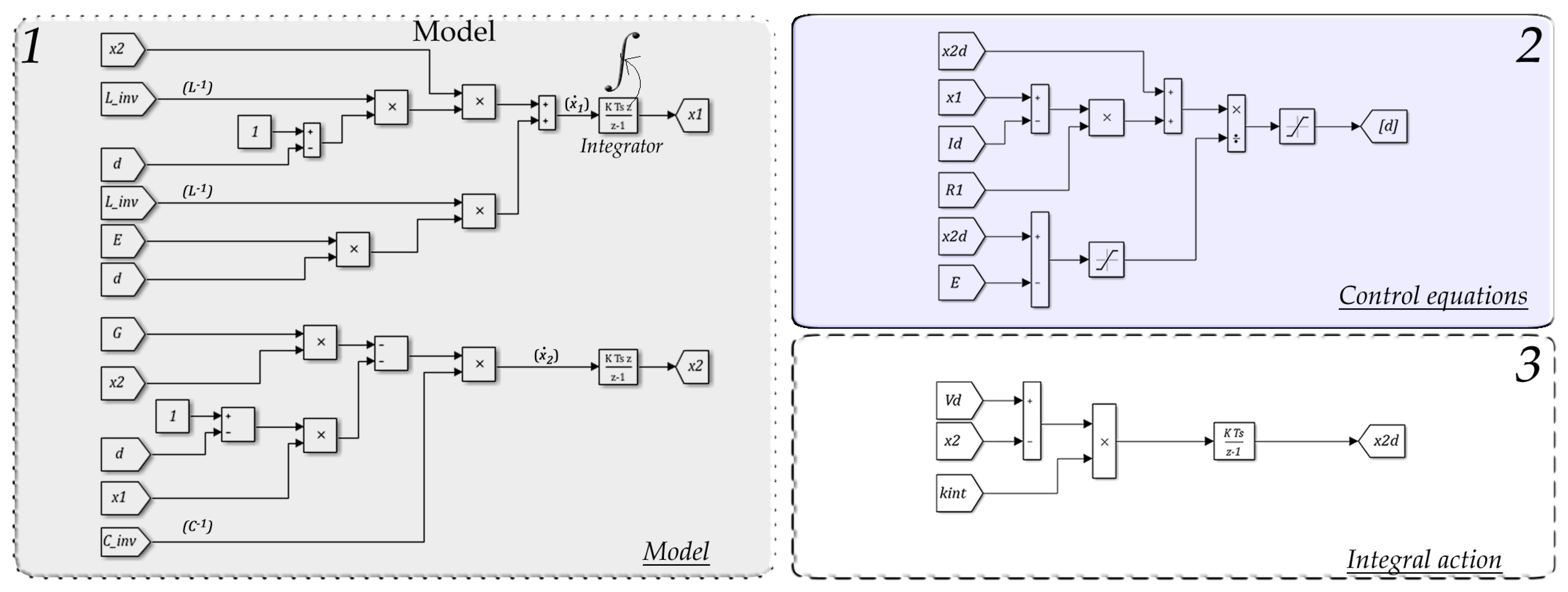
Figure 4 shows the overview of SHIL proposed methodology. The first step is obtaining the plant and the control equation models. After that, such models can be simulated using commonly softwares as Matlab or PSIM. As an example, Figure 4 illustrates the Flyback’s converter model and the SFL control equations, designed with Matlab/Simulink tools. Figure 5 shows the simulation in PSIM software. After the implementation, it is necessary to run the simulation and verify if the control and state variables are converging to the desired state. Once this is achieved, the next step is to embed the simulated system in the DSP. By using the external mode of Simulink and a compiler for the DSP, the model will be converted in code and then embedded to the target. Finally, the target will run the code, emulating the converter and control models. It is possible to verify desired signals in an oscilloscope by programming the DSP pins through DAC (Digital Analog Converter) blocks available in the $C2000$ $Texas$ $Instruments$ package. An important detail is the need of a scale adjustment for voltage compatibility between the simulation and target.

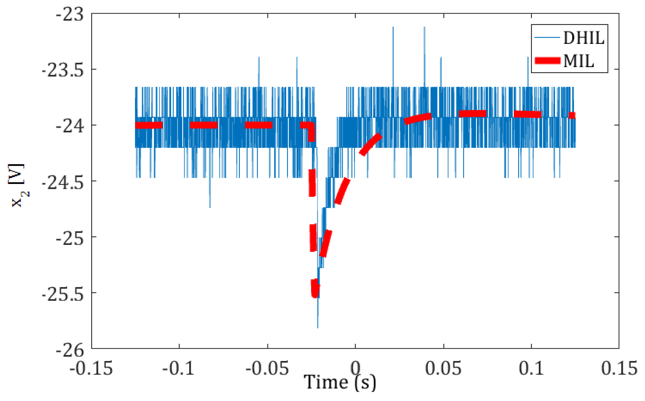
3.2. DHIL

With the proposed SHIL and DHIL methodologies, we can easily test the control law without needing a desktop computer or a real plant. In SHIL, the data transfer occurs directly and faster when both model and control are inserted in the same Digital Signal Processor. However, DHIL is best suited for synchronization, measurement and data communication tests between different systems.

The supporting package for C2000 microcontrollers available in Matlab/Simulink can be found in the Simulink library. Basic information about block functions, simulation configurations for real-time simulation or external mode and examples of systems implementation using the fundamental blocks such as PWM, ADC, DAC and interruptions can be found in Mathworks [33] website, or in Matlab “Help” area. Once selected, a list of C2000 DSP family will be displayed. By choosing the corresponding DSP, available blocks for the microcontroller are displayed. it is possible to build block systems with other Simulink blocks, by simply dragging them to the model window.

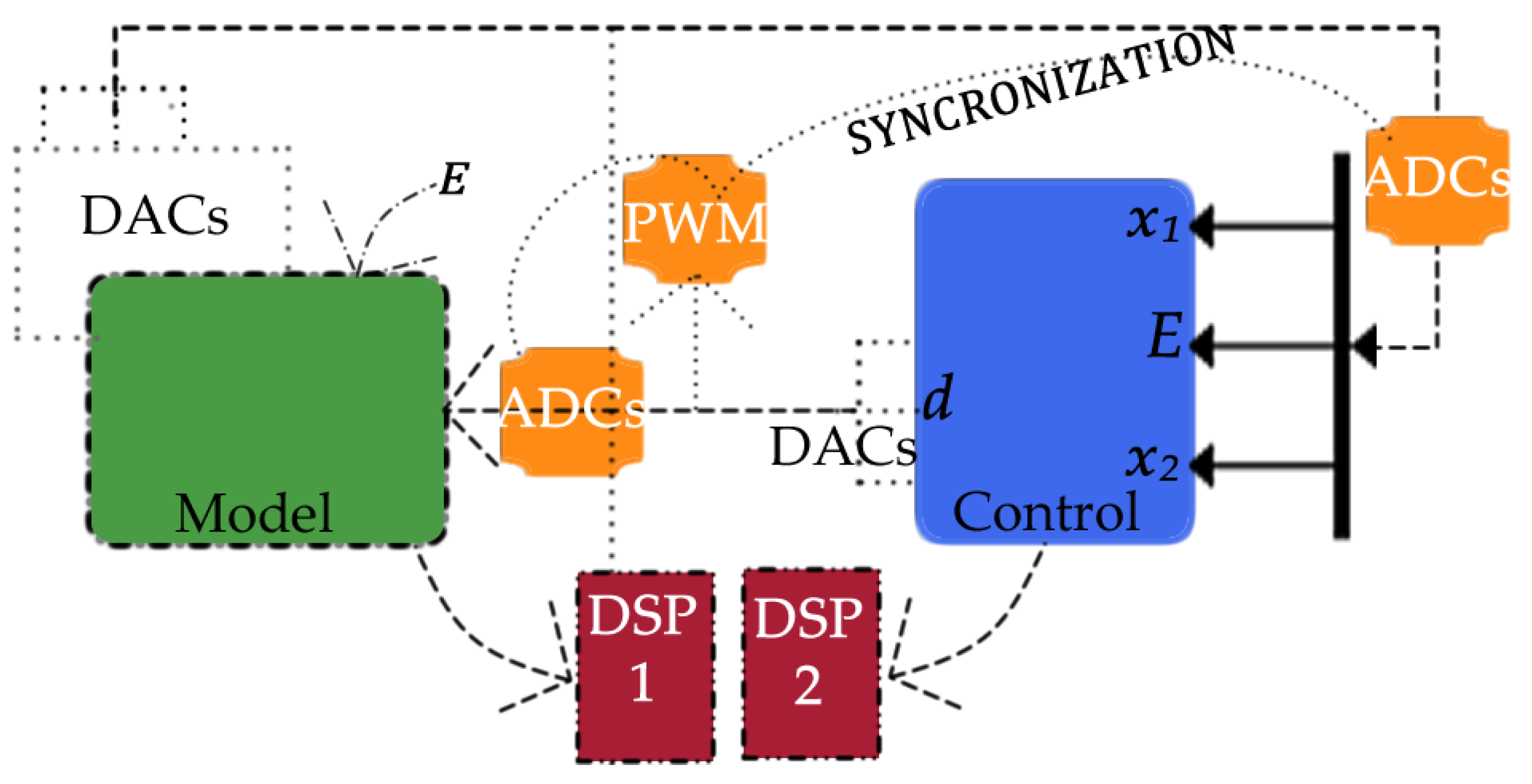
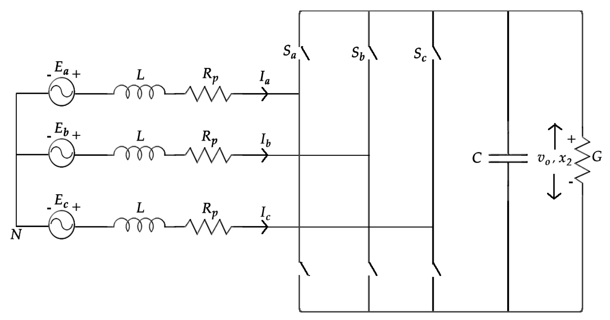
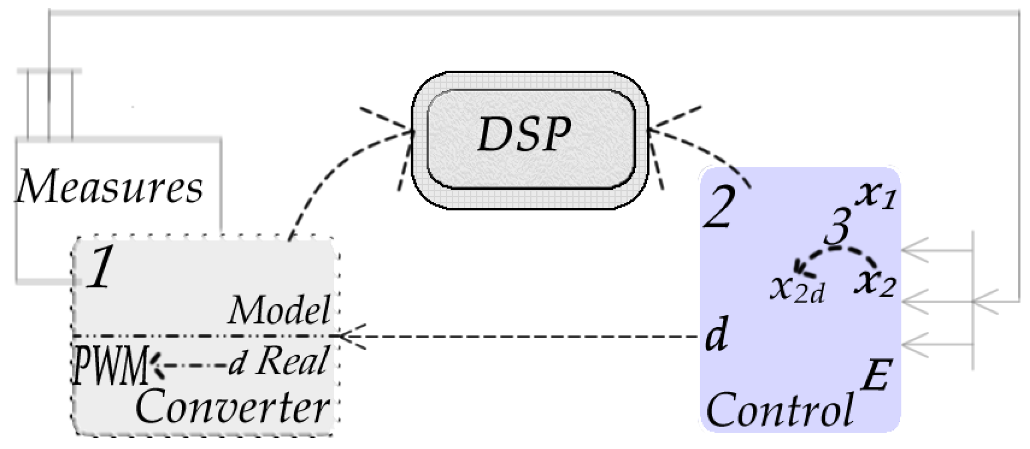
In DHIL, the use of a PWM (Pulse Width Modulation) block is necessary in order to control the converter switching sequence and also to synchronize 3 ADCs (Analog Digital Converter) available for measuring the inductor current ($x_1$), capacitor voltage ($x_2$) and the input voltage E. As seen in Figure 6, the control laws and the converter model are embedded in different microcontrollers. For computing the control laws, the inputs of the model are ($x_1$), ($x_2$) and E. Since those inputs are originated from the converter model computation—configured as analog signals type—it is necessary to convert those signals to a digital one, through analog-digital converter (ADC). After conversion, the output of the control law is the duty cycle. Since this control variable is digital, it will be converted to analog (DAC), for reading in the ADC of the DSP embedded with the converter model. For closing the loop, the variables ($x_1$), ($x_2$) and E are calculated and consequently converted from digital to analog type. It is important to notice that the conversions are based on the PWM sample rate, then requires the synchronization between both DSPs for a correct computation of control laws and converter model.

3.3. Details of the Implementation

Also, the approach used for programming the microcontroller diverges from the conventional one, being unnecessary the development of code lines. By using code generation tools and software libraries it is possible to resort the implementation of converter models and controllers through Matlab/Simulink blocks. The evident advantages of this approach are the clear visualization of the programming process and the time spared for development. 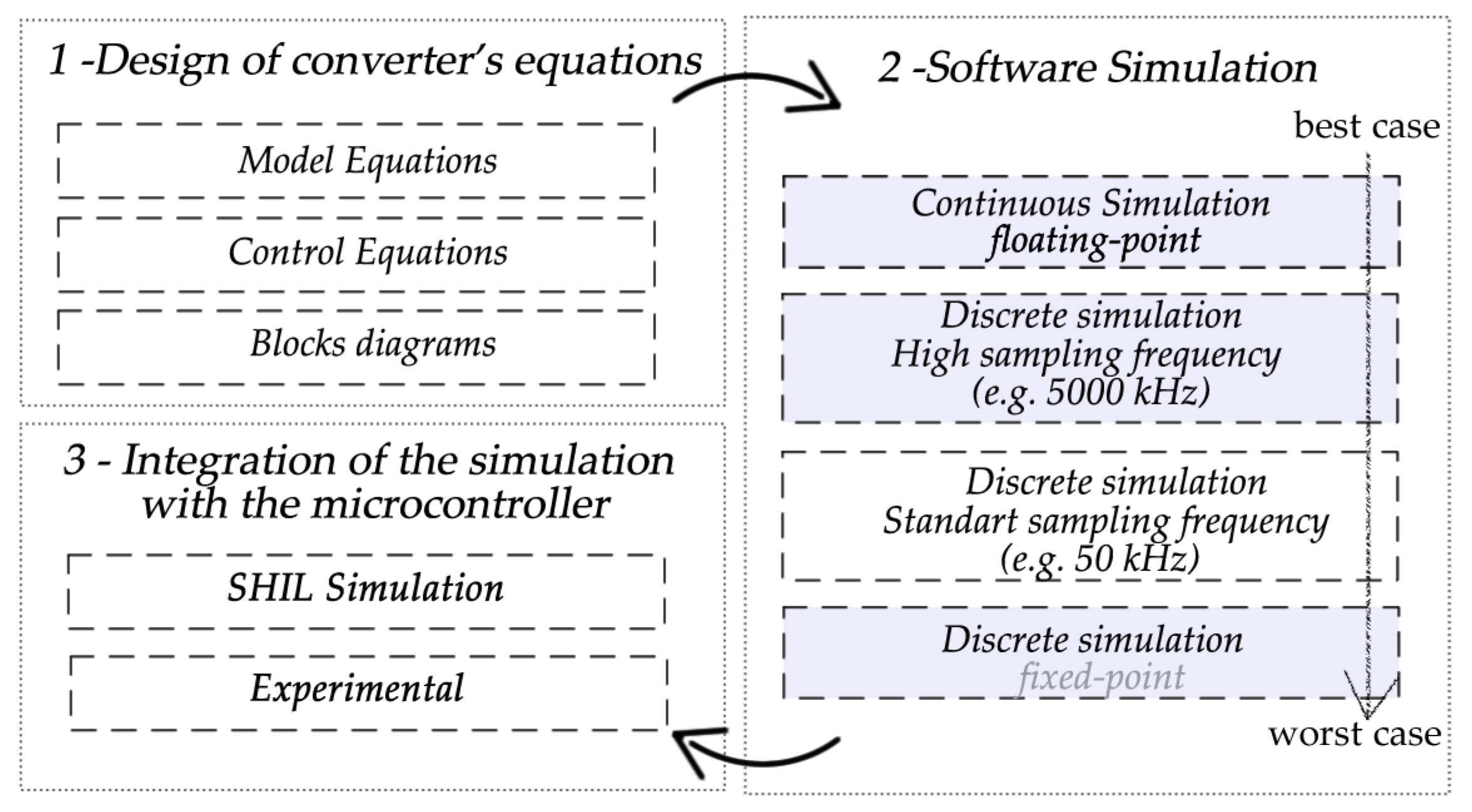Figure 7 illustrates the proposed steps for this methodology.

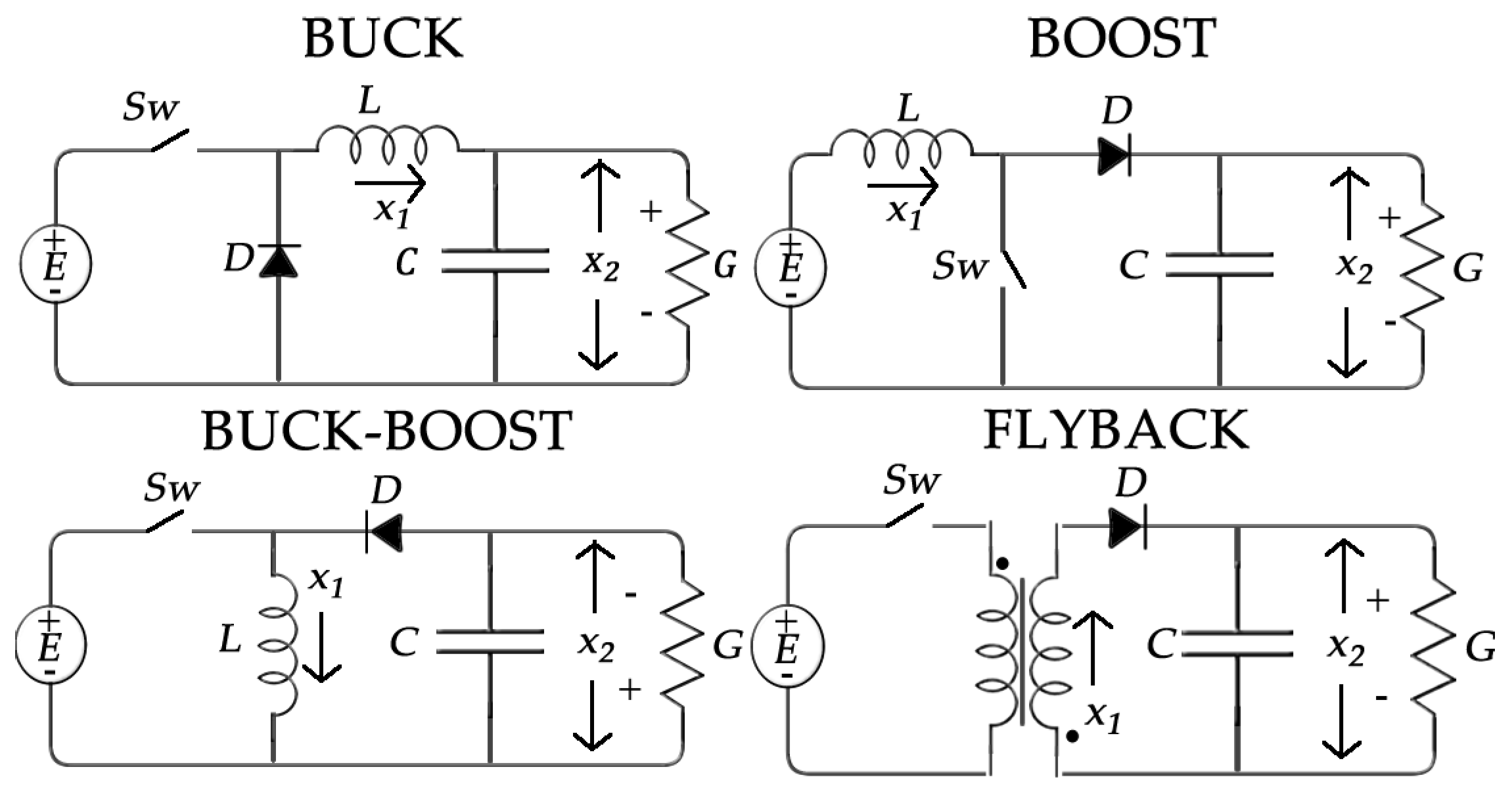
The first stage consists in developing an equation model for the system, demonstrating the relation between the state and control variables. It is up to the user to consider or not the nonlinearities of the system. Next, it is necessary to choose a control technique for actuating in the variable of interest. The nature of the control technique is wide, and can include since classical techniques, as PID controllers, to nonlinear control approaches. This stage ends with the implementation of the model and control equations in the simulation software. 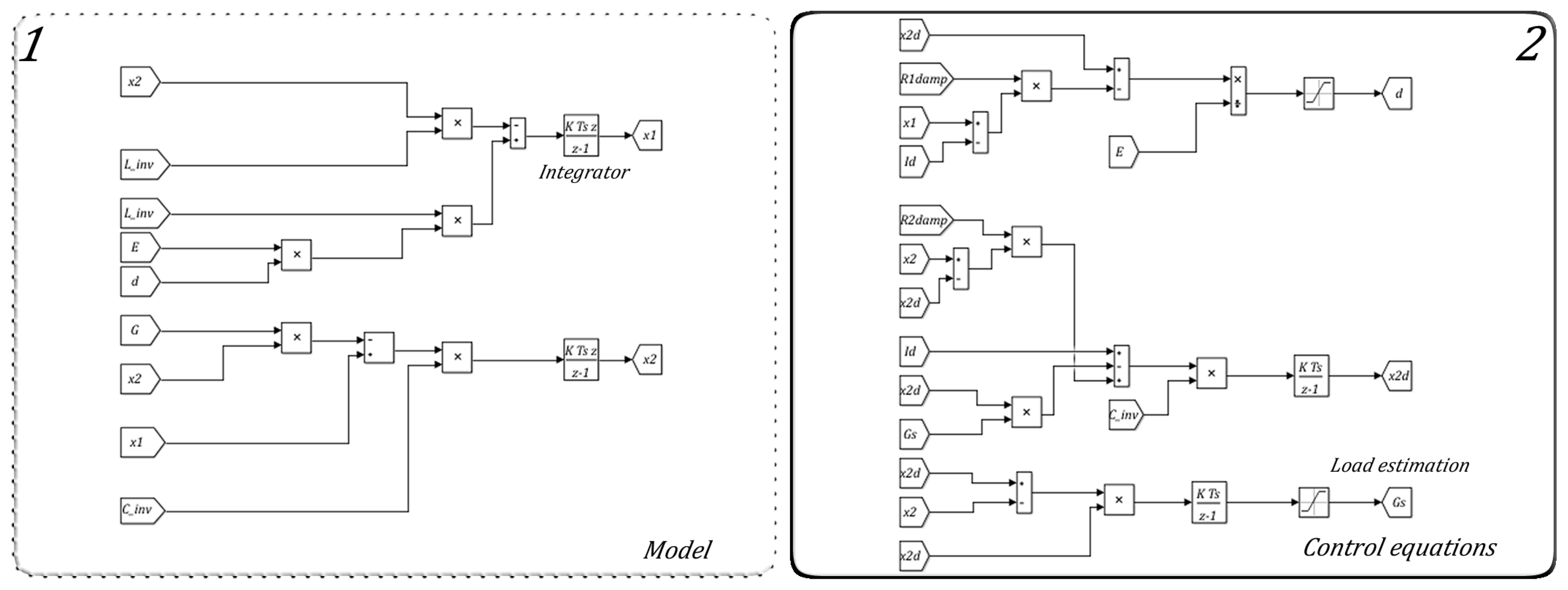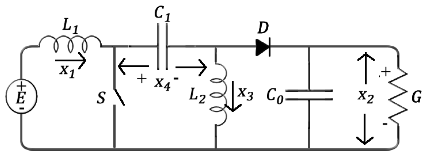Figure 8 presents the implemented model and control equations of a buck-boost converter, as an example. 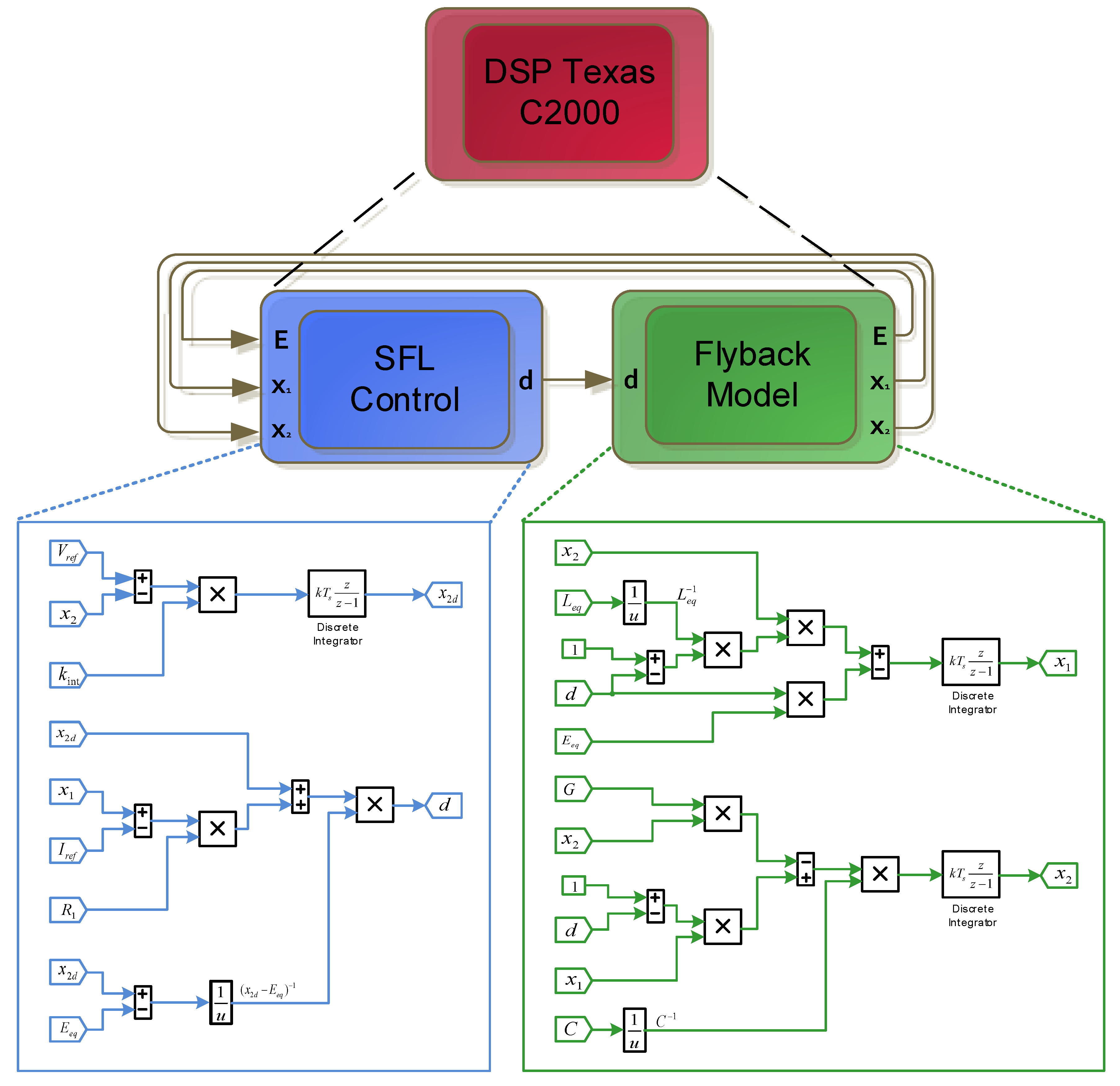Figure 9 shows the general SHIL simulation scheme for any converter. The main control goal is to calculate the duty cycle d(used in mathematical model), then the corresponding PWM signal is generated as an input control to command the switch of the physical converter. The state variables (inductor current x${}_1$ and voltage capacitor x${}_2$) and input voltage E are the required measures. An integral action is added to better regulate the output voltage.

The second phase consists of simulating the implemented system. Aiming at minimizing the errors, it is advised to simulate the system in continuous time and afterly in discrete time. For the continuous system it is important to work with float data type, by programming the operations of multiplication, division and constant blocks to “single/double” types. Although the increasing in processing time, this data type conversion configures one less source of error in the continuous time simulation.

After that, it is necessary to discretize the system, by changing the controllers structure and continuous operators to the corresponding discrete blocks (defining a sample time in which the blocks will be sampled). In a way to approach the results of the first discretized system to the continuous simulation it is proposed the use of a high sample frequency (or a small sample time).

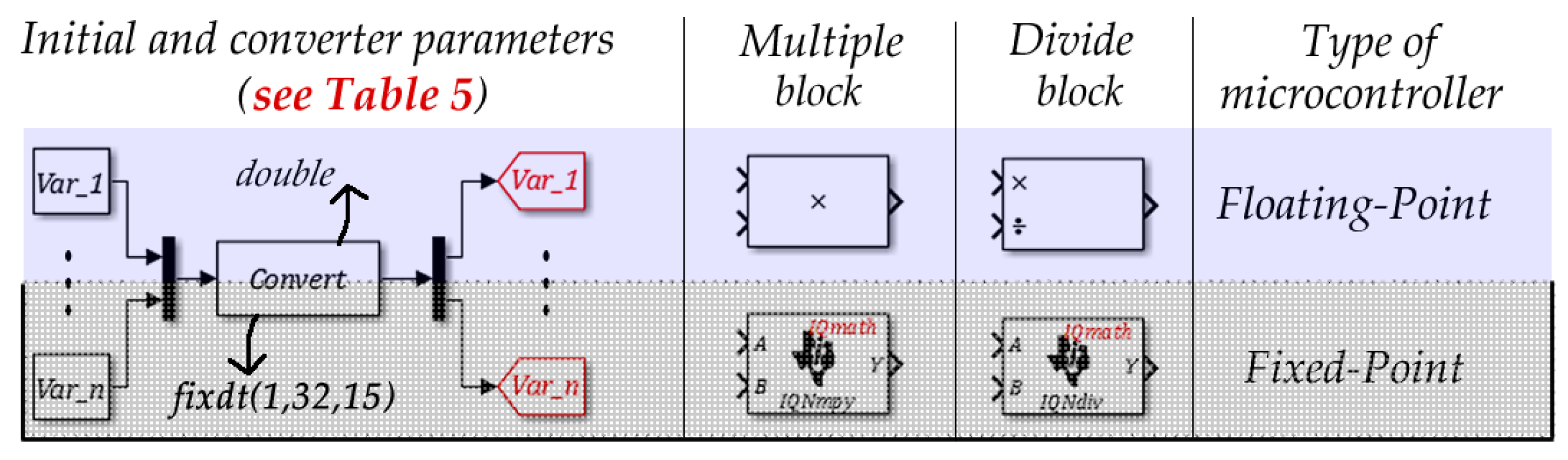
The next task is to simulate the system, considering a standard sample frequency (e.g., nominal 50 kHz), in such way to obtain a discrete model that is less approached by the continuous model. The selection of this frequency must be cautiously chosen, since the system can converge to instability. Another common problem associated to a bad choice of the sample frequency is the signal aliasing (Nyquist rule). The final objective of this stage consists in transforming the floating point data in fixed point data. This conversion can be done by programming the operations of multiplication, division and constant blocks to fixed-point type, or by using operational blocks offered in specific libraries for microcontrollers (libraries that are offered by Mathworks for users of C2000’s microcontrollers family, by Texas Instruments, for example), as shown in Figure 10. Some recomendations: avoid operations with floating data and divisions that increase the processing time. Always when possible, use multiplication operations instead of division operations (ex: when the denominator is a constant). Declare the variables as fixed point, preventing calculus with float and optmizing the code’s execution. Discrete models can be embedded for HIL simulation, since the user compiler can convert the blocks in code. However, a discrete model that converges, when working with fixed point data, makes the compilation and the processing time of the microcontroller smaller (and also the memory used smaller). In this way, the last step brings a discrete model more appropriated for a HIL procedure.

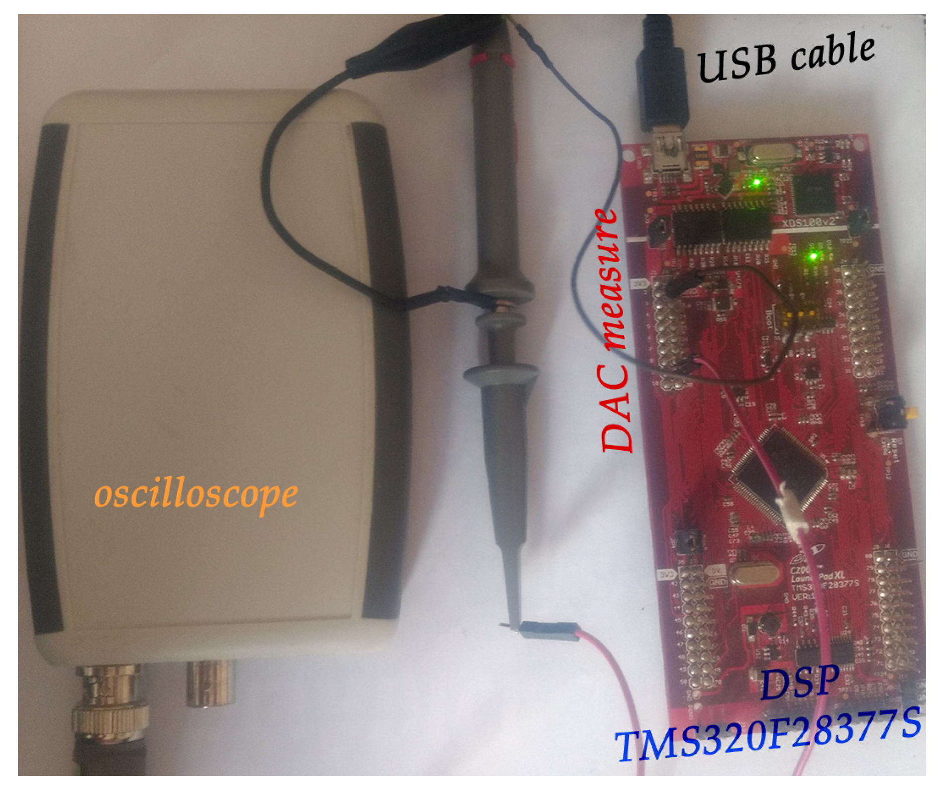
The final stage is the SHIL simulation itself. Once the compiler has generated the code and the system is embedded to the microcontroller (also called target) the communication between the target and the computer, in which Matlab/Simulink is running, begins. Usually microcontrollers of C2000 family communicates to the computer through USB or ethernet cable. In this application it is proposed the use of a USB cable. For running the system as a real-time simulation it is proposed to set the simulation as “external mode” simulation on Simulink. Also, it is necessary to set on the simulation configurations which target the connection must occur.

Since we are interested in plotting or viewing the gathered data, it is necessary to use specific blocks in the simulation for real-time plotting or setting DSP pins as analog outputs [33]. By doing that the user can see the data generated in the target in a Simulink “scope” or in an oscilloscope (by analog output reading). Each case can be achieved by using the RTDX (real-time Data Exchanged) or the DAC blocks, as seen in Figure 11. Since the R2016b version of Matlab there is a DAC block for DSP28377S of C2000 family (Texas Instruments). This block configures 3 digital inputs as 3 analog outputs (also called channels A, B and C). In this way it is possible to use 3 channels of an oscilloscope and view the curves in real-time.

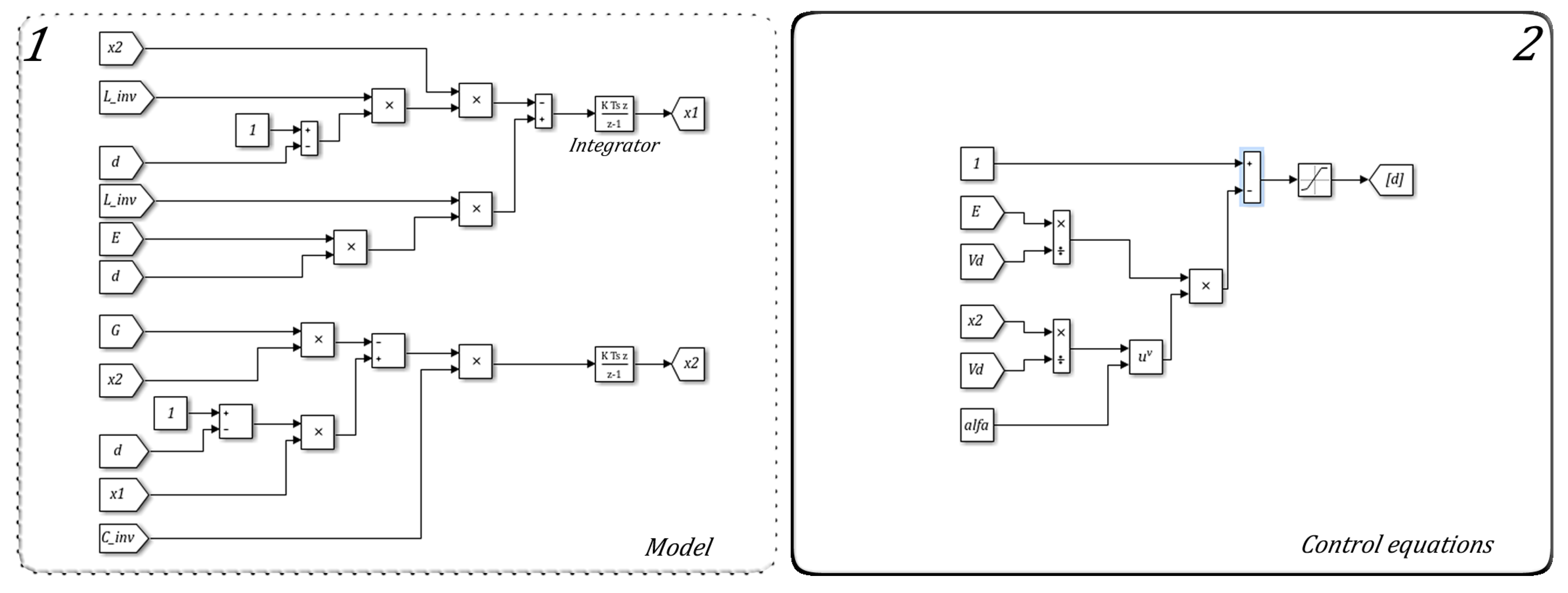
More details of the control algorithms implementation in block diagrams can be seen in the Figure 12 and Figure 13. Since the didactical background available in the literaute lacks of information, details of the functional blocks are shown, providing a development base for future works. Although the approach of this chapterdeals with a specific study of case, the available content makes it simple to adapt the program to other applications. General files, containing the control methods for Buck-Boost, Boost and Buck converters are shown in Figure 8, Figure 12 and Figure 13, respectively.

4. SHIL and DHIL Results for Buck-Boost and Flyback

This section shows the digital simulations using Matlab (Model in The Loop: MIL) and SHIL/DHIL experimental results. The converters are designed according to specifications listed on

Table 4. Initial and converters parameters.

Parameters	Buck-Boost	Flyback
$V_d$	−24 V	24 V
E	50 V	50 V
R	10 $\Omega$	11.5$\Omega$
L	0.6 mH	146 $\mathsf{\mu }$H, 35 $\mathsf{\mu }$H
C	470 $\mathsf{\mu }$F	470 $\mathsf{\mu }$F
$f_{sw}$	50 kHz	100 kHz
$R_{1damp}$ = $L{k}_1$	100	15
$k_{int}$	200	−5000

and the three control laws studied in this work. The experimental setup is sketched in Figure 14. The plots displayed in Figure 15a,c present the capacitor voltage response when an input voltage and a load variations, respectively, are included in the Buck-Boost converter simulated in software. The same effect is reported for the Flyback converter in Figure 15b,d. In both input and load variation, consecutive steps of 70% to 100% are applied in the simulated systems. An open-loop control test is also presented in Figure 16. Figure 17 and Figure 18 show the output capacitor voltage of Flyback and Buck-Boost converters, respectively, for the SHIL and DHIL applications. A load variation (70–100%) is applied for evaluate the three control laws.

It is possible to appreciate in the figures how the waveforms in both software and real-time simulations are compatibles. Although consecutive perturbations can be applied, the convergence of the variables to steady-state values is assured. In addition, similar transient dynamics can be observed, none of the implemented systems in software or in HIL present instability. Therefore, the embedded models and control equations are validated. The processing time for the DSP to compute the control law and converter state, and therefore to run a real-time simulation, is 1.2 $\mathsf{\mu }$s.

5. SHIL Results for Second Order Power Converters and Comparison

This section presents the digital simulation results using Matlab and SHIL method for buck, boost and buck-boost. The converters are implemented according to design specifications of

Table 5. Initial and converters parameters.

Parameters	Boost	Buck	Buck-Boost
$I_d$	$\frac{G}{E}{V}_d^2$	$G{V}_d$	${GV}_d(\frac{V_d}{E}-1)$
R	52.5 $\Omega$	10 $\Omega$	10 $\Omega$
L	0.6 mH	0.6 mH	0.6 mH
C	2800 $\mathsf{\mu }$F	470 $\mathsf{\mu }$F	470 $\mathsf{\mu }$F
E	100 V	50 V	50 V
V${}_d$	180 V	24 V	−24 V
Pout	630 W	57.6 W	57.6 W
f	50 kHz	50 kHz	50 kHz
R${}_{1damp}$	33	500	100
R${}_{2damp}$	50	0	0
k${}_g$	0.0356	2.5	14
k${}_{int}$	−150	2000	200
$\alpha$	0.8	−10	0.8

and the three control laws studied in this work. Figure 19 shows the capacitor voltage response to a load voltage variation (70% G to 100% G), respectively, in the converters simulated in software. Figure 20 shows the capacitor voltage of the converters for the SHIL application. A load variation (70–100%) is applied to evaluate the three control laws. Figure 21 shows the PWM signal generated in HIL simulation for the buck-boost converter in steady state operation.

As seen in the figures, both software simulations and SHIL results converged to the steady state value after the consecutive step applications. It should be noticed that the dynamical response of the systems is compatible, since the same transient dynamics is seen, even for the IDA-PBC’s oscillatory dynamics. None of the implemented systems in software or in SHIL presented instability. Therefore, it means that the embedded models and control equations are capable in controlling the systems, and therefore, validating the control techniques.

In general, the SFL, PBC and IDA-PBC control laws show satisfactory results for the three types of converters studied: boost, buck and buck-boost. It was observed that the inductor current and output voltage in the capacitor, the main variables, follow the reference set points, reaching the control objectives. Since one of the main objectives of this work is the comparison of control methods,

Table 6. Comparison of non linear control methods.

Comparison	SFL		PBC		IDA-PBC
	Advantage	Disadvantage	Advantage	Disadvantage	Advantage	Disadvantage
Control law	simple			medium	open loop
Solution	easy			medium complexity		Nontrivial
Parameters	2			4	1
Measurements		3		3	2
AC-DC System	low THD levels and high PF		low THD levels and high PF			incorrectly, high THD rates
Control Type		direct control is only for the buck		direct control is only for the buck	Direct control is possible for all
Integral term	Soft integration		Soft integration			very sensitive
Dependence on realistic model		medium		medium		very dependent on realistic mode
Parametric dependence control	Does not depend on C			It depends on the G, L and C.	Control law does not depend on G, L or C
Processing Time (TMS320F2812 fixed-point DSP)	Fast (2.4 $\mathsf{\mu }$s)		Fast (3.2 $\mathsf{\mu }$s)		Fast (6 $\mathsf{\mu }$s)
Processing Time (TMS320F28377S floating-point DSP)	Fast (1.2 $\mathsf{\mu }$s)		Fast (1.2 $\mathsf{\mu }$s)		Fast (1.2 $\mathsf{\mu }$s)
sum	4			8	3
div	1			1	0
mult	3			6	3
other operation						1 (exp)
Load Estimation		Cannot estimate by the output voltage error.	Can estimate the load by voltage error		It is not necessary estimate the load

shows, from an implementation point of view, the advantages and disadvantages of each method.

It is seen that SFL and PBC present similar results. Reminding that, for both control techniques the indirect control is the only possibility [10]. On one hand the SFL is a didactic and easier solution than the PBC. On the other hand, the control complexity of PBC is justified for load estimation and better voltage output regulation. However, there is a trade-off, since the overshoot and undershoot increase with the adaptative control law and the integral gain used.

SFL and PBC control present small error in steady state for the output voltage of the capacitor, without the integral action. On the other hand, the IDA-PBC control presented larger overshoot/ undershoot and accommodation times, notably for input voltage variations. This is because this technique is even more dependent on the exact knowledge model parameters. Thus, to improve the results it is necessary to include other non-modeled effects like parasitic resistances, diode and switches voltage drops [34].

Once IDA-PBC control is a direct control, it does not require the measurement of the current $x_1$, which is an advantage in terms of implementation. In general terms, we can verify:

-

SFL: simpler, didactic, effective, dispenses load estimation for DC-DC systems when using integrative gain.

-

PBC: has medium complexity, needs more measurements and control parameters to better estimate the load and regulate the output capacitor voltage. It is the most recommended technique for PFC systems, since it offers lower THD levels [13]. It has the same processing time as the SFL control because of the same amount of division operations, which effectively determine the total processing time (sums and multiplications offer irrelevant contributions).

-

IDA-PBC: non-trivial control solution, allows direct control, which exempts current measurement and eventual problems. By the same direct nature of the control, does not work correctly for AC-DC systems, since the objective is to impose the current in phase with grid input voltage.

6. Conclusions

This work showed the buck, boost, buck-boost, flyback, SEPIC and 3-phase AC/DC boost converters modeling as well as the development of nonlinear control techniques using SHIL and DHIL implementations. In addition, the control and converter models were implemented in a DSP, resulting in a quick and cheap HIL realization of the proposed systems, ideal for students and engineers interested in learning and validating converters performance. Using a switching frequency of 50 kHz (20 $\mathsf{\mu }$s), the processing time of the model/control equations (1.2 $\mathsf{\mu }$s) demands 6% of the bandwidth (for buck, boost, buck-boost, flyback and SEPIC). According to the data in Table 6, there is a clear preference for new embedded systems with floating-point operation. As illustrated in Figure 16 and Figure 18 and despite measurement noises, the SHIL/DHIL results remained close to the model-simulated one. The advantages provided by the proposed method are: security, saving development time, facilitating the understanding of the programming process, standardization, concurrent simulation, rapid prototyping and, mainly, an easy and cheap way to validate linear and nonlinear controllers.

References

1. Shoushtari, M.; Dutt, N. SAM: Software-Assisted Memory Hierarchy for Scalable Manycore Embedded Systems. IEEE Embed. Syst. Lett. 2017, 9, 109–112. [Google Scholar] [CrossRef]
2. Noureen, S.; Shamim, N.; Roy, V.; Bayne, S. real-time Digital Simulators: A Comprehensive Study on System Overview, Application, and Importance. Int. J. Res. Eng. 2017, 4, 266–277. [Google Scholar] [CrossRef]
3. Grégoire, L.; Cousineau, M.; Seleme, S., Jr.; Ladoux, P. real-time Simulation of Interleaved Converters with Decentralized Control. In Proceedings of the International Conference on Renewable Energies and Power Quality (ICREPQ 2016), Madrid, Spain, 4–6 May 2016; pp. 1–6. [Google Scholar]
4. Li, Y.; Xu, X.; Sun, X.; Xue, H.; Jiang, H.; Qu, Y. Theoretical and experimental analytical study of powertrain system by hardware-in-the-loop test bench for electric vehicles. Int. J. Veh. Syst. Model. Test. 2017, 12, 44–71. [Google Scholar] [CrossRef]
5. Fernández-Álvarez, A.; Portela-García, M.; García-Valderas, M.; López, J.; Sanz, M. HW/SW Co-Simulation System for Enhancing Hardware-in-the-Loop of Power Converter Digital Controllers. IEEE J. Emerg. Sel. Top. Power Electron. 2017, 5, 1779–1786. [Google Scholar] [CrossRef]
6. Vardhan, H.; Akin, B.; Jin, H. A Low-Cost, High-Fidelity Processor-in-the Loop Platform: For Rapid Prototyping of Power Electronics Circuits and Motor Drives. IEEE Power Electron. Mag. 2016, 3, 18–28. [Google Scholar] [CrossRef]
7. Motahhir, S.; El Ghzizal, A.; Sebti, S.; Derouich, A. MIL and SIL and PIL tests for MPPT algorithm. Cogent Eng. 2017, 4, 1378475. [Google Scholar] [CrossRef]
8. Bélanger, J.; Venne, P.; Paquin, J. The What, Where and Why of Real-Time Simulation. Available online: https://www.opal-rt.com/wp-content/themes/enfold-opal/pdf/L001610436.pdf (accessed on 1 June 2018).
9. Erickson, R.W.; Maksimovic, D. Fundamentals of Power Electronics; Springer Science & Business Media: New York, NY, USA, 2007. [Google Scholar]
10. Sira-Ramirez, H.; Perez-Moreno, R.A.; Ortega, R.; Garcia-Esteban, M. Passivity-based controllers for the stabilization of DC-to-DC power converters. Automatica 1997, 33, 499–513. [Google Scholar] [CrossRef]
11. Sanders, S.R. Nonlinear Control of Switching Power Converters. Ph.D. Thesis, Massachusetts Institute of Technology, Cambridge, MA, USA, 1989. [Google Scholar]
12. Rosa, A.H.R. Estudo e Comparação de Técnicas de Controle não Lineares Aplicadas a Conversores Estáticos de Potência. Ph.D. Thesis, UFMG, Belo Horizonte, Brazil, 2015. [Google Scholar]
13. Seleme, S.I.; Rosa, A.H.R.; Morais, L.M.F.; Donoso-Garcia, P.F.; Cortizo, P.C. Evaluation of adaptive passivity-based controller for power factor correction using a boost converter. IET Control Theory Appl. 2012, 6, 2168–2178. [Google Scholar] [CrossRef]
14. Rosa, A.; Morais, L.M.; Seleme, I. A study and comparison of nonlinear control techniques apply to second order power converters using HIL simulation. In Proceedings of the 2016 12th IEEE International Conference on Industry Applications (INDUSCON), Curitiba, Brazil, 20–23 November 2016; pp. 1–8. [Google Scholar]
15. Wang, Y.; Yu, H.; Yu, J. The modeling and control of buck-boost converter based on energy-shaping theory. In Proceedings of the IEEE International Conference on Industrial Technology (ICIT 2008), Chengdu, China, 21–24 April 2008; pp. 1–6. [Google Scholar]
16. Ortega, R.; Garcia-Canseco, E. Interconnection and damping assignment passivity-based control: A survey. Eur. J. Control 2004, 10, 432–450. [Google Scholar] [CrossRef]
17. Ortega, R.; Van Der Schaft, A.; Maschke, B.; Escobar, G. Interconnection and damping assignment passivity-based control of port-controlled Hamiltonian systems. Automatica 2002, 38, 585–596. [Google Scholar] [CrossRef] [Green Version]
18. Raviraj, V.; Sen, P.C. Comparative study of proportional-integral, sliding mode, and fuzzy logic controllers for power converters. IEEE Trans. Ind. Appl. 1997, 33, 518–524. [Google Scholar] [CrossRef] [Green Version]
19. Fu, J.; Jin, Y.; Zhao, J. Nonlinear control of power converters: A new adaptive backstepping approach. Asian J. Control 2009, 11, 653–656. [Google Scholar] [CrossRef]
20. Beccuti, A.G.; Papafotiou, G.; Morari, M. Explicit model predictive control of the boost dc-dc converter. IFAC Proc. Vol. 2006, 39, 315–320. [Google Scholar] [CrossRef]
21. Almér, S.; Mariéthoz, S.; Morari, M. Piecewise affine modeling and control of a step-up DC-DC converter. In Proceedings of the American Control Conference (ACC), Baltimore, MD, USA, 30 June–2 July 2010; pp. 3299–3304. [Google Scholar]
22. Morais, L.M.F.; Santos Filho, R.M.; Cortizo, P.C.; Seleme, S.I.; Garcia, P.F.D.; Seixas, P.F. Pll-based repetitive control applied to the single-phase power factor correction using boost converter. In Proceedings of the 35th Annual Conference of IEEE Industrial Electronics (IECON’09), Porto, Portugal, 3–5 November 2009; pp. 737–742. [Google Scholar]
23. Kancherla, S.; Tripathi, R. Nonlinear average current mode control for a DC-DC buck converter in continuous and discontinuous conduction modes. In Proceedings of the 2008 IEEE Region 10 Conference (TENCON 2008), Hyderabad, India, 19–21 November 2008; pp. 1–6. [Google Scholar]
24. He, W.; Ortega, R.; Machado, J.E.; Li, S. An Adaptive Passivity-Based Controller of a Buck-Boost Converter with a Constant Power Load. arXiv, 2017; arXiv:1712.07792. [Google Scholar] [CrossRef]
25. Khalil, H.K. Noninear Systems; Prentice-Hall: Upper Saddle River, NJ, USA, 1996. [Google Scholar]
26. El Aroudi, A.; Giaouris, D.; Iu, H.H.; Hiskens, I. A review on stability analysis methods for switching mode power converters. IEEE J. Emerg. Sel. Top. Circuits Syst. 2015, 5, 302–315. [Google Scholar] [CrossRef]
27. Sira-Ramírez, H.; Ortega, R.; García-Esteban, M. Adaptive passivity-based control of average dc-to-dc power converter models. Int. J. Adapt. Control Signal Proc. 1998, 12, 63–80. [Google Scholar] [CrossRef]
28. Hosseinzadeh, M.; Yazdanpanah, M.J. Robust adaptive passivity-based control of open-loop unstable affine non-linear systems subject to actuator saturation. IET Control Theory Appl. 2017, 11, 2731–2742. [Google Scholar] [CrossRef]
29. Seker, M.; Zergeroglu, E. Nonlinear control of flyback type DC to DC converters: An indirect backstepping approach. In Proceedings of the 2011 IEEE International Conference on Control Applications (CCA), Denver, CO, USA, 28–30 September 2011; pp. 65–69. [Google Scholar]
30. Rosa, A.; Silva, M.; Campos, M.; Santana, R.; Cortizo, P.; Mendes, M.; Morais, L.; Seleme, I. Hil simulation of non linear control methods applied for buck-boost and flyback converters. In Proceedings of the 2017 Brazilian Power Electronics Conference (COBEP), Juiz de Fora, Brazil, 19–22 November 2017; pp. 1–6. [Google Scholar]
31. Zhang, M.; Borja, P.; Ortega, R.; Liu, Z.; Su, H. PID Passivity-Based Control of Port-Hamiltonian Systems. IEEE Trans. Autom. Control 2018, 63, 1032–1044. [Google Scholar] [CrossRef]
32. Balluchi, A.; Benvenuti, L.; Engell, S.; Geyer, T.; Johansson, K.H.; Lamnabhi-Lagarrigue, F.; Lygeros, J.; Morari, M.; Papafotiou, G.; Sangiovanni-Vincentelli, A.L.; et al. Hybrid control of networked embedded systems. Eur. J. Control 2005, 11, 478–508. [Google Scholar] [CrossRef]
33. Parameter Tuning and Signal Logging with Serial External Mode. Document Description. Available online: https://www.mathworks.com/help/supportpkg/texasinstrumentsc2000/examples/parameter-tuning-and-signal-logging-with-serial-external-mode.html (accessed on 30 May 2017).
34. Márquez-Contreras, R.; Rodríguez-Cortés, H.; Spinetti-Rivera, M. Revisiting IDA-PBC, Open-Loop Control, and Modeling for the Boost DC-DC Power Converter. In Proceedings of the Latin American Congress of Automatic Control, Rio de Janeiro, Brazil, 5–6 November 2008. [Google Scholar]
35. Sira-Ramirez, H.; deNieto, M.D. A Lagrangian approach to average modeling of pulsewidth-modulation controlled DC-to-DC power converters. IEEE Trans. Circuits Syst. I Fundam. Theory Appl. 1996, 43, 427. [Google Scholar] [CrossRef]
36. Stadlmayr, R.; Schlacher, K. An energy-based control strategy for DC/DC power converters. In Proceedings of the 2009 European Control Conference (ECC), Budapest, Hungary, 23–26 August 2009; pp. 3967–3972. [Google Scholar]
37. Yildiz, H.A.; Goren-Sumer, L. Lagrangian modeling of DC-DC buck-boost and flyback converters. In Proceedings of the European Conference on Circuit Theory and Design (ECCTD 2009), Antalya, Turkey, 23–27 August 2009; pp. 245–248. [Google Scholar]
38. Seleme, S.I., Jr.; Morais, L.M.F.; Rosa, A.H.R.; Torres, L.A.B. Stability in passivity-based boost converter controller for power factor correction. Eur. J. Control 2013, 19, 56–64. [Google Scholar] [CrossRef]
39. Rodriguez, H.; Ortega, R.; Escobar, G. A new family of energy-based non-linear controllers for switched power converters. In Proceedings of the IEEE International Symposium on Industrial Electronics (ISIE 2001), Pusan, Korea, 12–16 June 2001; Volume 2, pp. 723–727. [Google Scholar]
40. Ma, H.; Li, Y.; Lai, J.; Zheng, C.; Xu, J. An Improved Bridgeless SEPIC Converter without Circulating Losses and Input Voltage Sensing. IEEE J. Emerg. Sel. Top. Power Electron. 2018, 6, 1447–1455. [Google Scholar] [CrossRef]
41. Zhang, M.; Ortega, R.; Liu, Z.; Su, H. A new family of interconnection and damping assignment passivity-based controllers. Int. J. Robust Nonlinear Control 2017, 27, 50–65. [Google Scholar] [CrossRef]
42. Rosa, A.; de Souza, T.; Morais, L.; Seleme, S., Jr. Adaptive and Nonlinear Control Techniques Applied to SEPIC Converter in DC-DC, PFC, CCM and DCM Modes Using HIL Simulation. Energies 2018, 11, 602. [Google Scholar] [CrossRef]
43. Lee, T.S. Lagrangian modeling and passivity-based control of three-phase AC/DC voltage-source converters. IEEE Trans. Ind. Electron. 2004, 51, 892–902. [Google Scholar] [CrossRef]
44. Rodriguez, L.; Jones, V.; Oliva, A.R.; Escobar-Mejía, A.; Balda, J.C. A new SST topology comprising boost three-level AC/DC converters for applications in electric power distribution systems. IEEE J. Emerg. Sel. Top. Power Electron. 2017, 5, 735–746. [Google Scholar] [CrossRef]
45. Rosa, A.; Morais, L.; Seleme, S., Jr. Practical hybrid solutions based on nonlinear controllers applied to PFC boost converter. Przeglkad Elektrotech. 2018, 1, 10–16. [Google Scholar] [CrossRef]
46. Rodrigues, W.; Oliveira, T.; Morais, L.; Rosa, A. Voltage and Power Balance Strategy without Communication for a Modular Solid State Transformer Based on Adaptive Droop Control. Energies 2018, 11, 1802. [Google Scholar] [CrossRef]
Figure 1. SHIL and DHIL.
Electronics 07 00241 g001
Figure 2. Basic power converters circuits.
Electronics 07 00241 g002
Figure 3. Models associated with non-linear control techniques.
Electronics 07 00241 g003
Figure 4. Flyback model, Equations (8) and (9), and SFL control Equation (10) in block diagrams (high level programing) that is embedded in DSP C2000.
Electronics 07 00241 g004
Figure 5. Simulation of flyback switched model using PSIM software. Normalized output voltage x 2 for load perturbation with a fixed time step 100 times smaller than the switching period. SFL (red), PBC (green) and IDAPBC (blue).
Electronics 07 00241 g005
Figure 6. DHIL.
Electronics 07 00241 g006
Figure 7. Methodology steps for SHIL simulation. The optional steps are highlighted in gray.
Electronics 07 00241 g007
Figure 8. Buck-boost model and SFL control equations in block diagrams. Model (1), control Equation (2) and integral action (3).
Electronics 07 00241 g008
Figure 9. General SHIL Simulation Scheme.
Electronics 07 00241 g009
Figure 10. Fixed-point and Floating-point different implementations.
Electronics 07 00241 g010
Figure 11. DAC Block: Used for showing state and internal variables in a scale between 0 V–3.3 V (12-bit resolution).
Electronics 07 00241 g011
Figure 12. Boost model and IDA-PBC control equations in block diagrams.
Electronics 07 00241 g012
Figure 13. Buck model and PBC control equations in block diagrams.
Electronics 07 00241 g013
Figure 14. Experimental setup.
Electronics 07 00241 g014
Figure 15. Software simulation result for Buck-Boost (a,c) and Flyback (b,d) (using control techniques SFL (red), PBC (blue) and IDA-PBC (green). Output voltage x 2 for input voltage (a,b) and for load variation (c,d).
Electronics 07 00241 g015
Figure 16. Open loop control comparing SHIL (blue line) with Software Simulation (red line) results for Buck-Boost converter. Normalized output voltage x 2 for load perturbation (70–100%) using fixed d = 0.325 .
Electronics 07 00241 g016
Figure 17. SHIL experimental result for Flyback (A) and Buck-boost (B) converters. Normalized output voltage x 2 for load perturbation (70–100%).
Electronics 07 00241 g017
Figure 18. DHIL experimental compared with Software Simulation (MIL) result for Buck-Boost converter (SFL control). Normalized output voltage x 2 for load perturbation (70–100%).
Electronics 07 00241 g018
Figure 19. Software simulation result using control techniques SFL (red), PBC (blue) and IDA-PBC (green). Output voltage x 2 for buck (a) and boost PFC (b); buck-boost (c) for load variation in 0.25 s and 0.75 s.
Electronics 07 00241 g019
Figure 20. SHIL experimental result. Normalized output voltage x 2 for load perturbation (70–100%).
Electronics 07 00241 g020
Figure 21. PWM signal generated in SHIL Simulation for buck-boost permanent condition (d = 0.37).
Electronics 07 00241 g021