1. Introduction
Any city management department is interested in detecting unusual events in the urban area as early as possible. Being aware of any unexpected situation going on in the city allows city management departments to take action, for instance by controlling traffic or public transportation or informing the city inhabitants. Many of the detection techniques are based on noticing the unexpected behavior of groups of people (e.g., abnormally high or low number of citizens) using cameras or other advanced devices in smart cities. The main drawback of this approach is the need to deploy a specialized physical infrastructure in the area under study.
To overcome this limitation, location-based social networks (LBSNs) seem to be an interesting approach: no specific infrastructure is needed to collect the data, but the citizens themselves are the ones who buy, maintain, and carry the needed mobile devices; and they freely disclose their location throughout the day by proactively posting pictures or tweets, thus making the process seamless to them. This paradigm allows collecting a high volume of data, coming from many different users, distributed throughout all the city, thus becoming a good proxy for representing the behavior of the city. However, collecting the continuous stream of LBSN data, summarizing and analyzing it, and actually detecting the anomalies are tasks that may lead to an important computational cost, thus making it difficult to be applied in real time.
With this trade-off in mind, we propose a novel approach to detect potential anomalies as they happen with an efficient methodology. The idea is to sample at intervals the location data of Instagram posts to represent the behavior of citizens. The collected locations at each interval will be summarized by their centroid. The novelty of our work relies on the use of entropy to analyze the sequence of centroid locations (one per interval) in order to detect anomalies. Since entropy measures the uncertainty of the next event in a sequence, when something unusual happens and the citizens’ locations greatly vary, we expect changes in the value of entropy.
This approach is shown to be quick enough to spot changes in the city behaviors as they happen, since entropy calculation is an easy iterative process. Although entropy has been traditionally used for outlier detection in many areas, to our knowledge, there are no previous approaches applying this strategy to detect crowd dynamics anomalies in urban areas. In this paper, we propose how to go from location information of a crowd to a sequence of symbols to which Shannon’s entropy definition can be applied.
The rest of the paper is as follows:
Section 2 overviews other alternatives to detect anomalies in crowd behavior, whereas our approach is detailed in
Section 3; after that, we present the data set and how the parameters of the algorithm are selected in
Section 4. In
Section 5, we validate the entropy-based methodology for crowd anomalies detection in the city. In
Section 6, we discuss the limitations of our approach. Finally, we discuss the conclusions in
Section 7.
2. Related Work
Early detection of unusual events in urban areas is a challenge that has been tackled from different sides. Besides the video-processing techniques [
1,
2], the use of public posts shared in social media has recently constituted a novel focus of attention [
3]. Some approaches focus on the shared content, for example the analysis of text messages to detect events, like in [
4] or [
5], where Twitter and Instagram were the data sources. Other proposals go further and try to detect natural disasters, such as earthquakes [
6] or forest fires [
7].
However, users’ locations are becoming more important, especially since LBSNs are so popular. In [
8], tweets were collected and assigned to previously-defined regions in intervals of six hours, which makes the possibility of the early detection of events difficult. Twitter was also used in [
9], where a high activity triggers the system. Later, those tweets were analyzed to know if the event was already expected or not. In this case, the detection does not work for low activity behaviors, even if they are rare indeed. The proposal in [
10] tried to detect and monitor local social events by applying clustering (k-means), although this technique requires specifying the number of cluster in advance, which is not flexible enough for detection purposes.
Previous work also faced crowd detection based on geolocated posts by using density-based clustering [
11,
12] without imposing an a priori decision about the number of clusters or their shape. In spite of having obtained sound and accurate results, its computation cost suggests applying this approach only when other evidence of unexpected behavior has been detected.
All works above face the problem of identifying events that do not match an expected pattern, which is established by applying both supervised or unsupervised machine learning approaches. Once a regular pattern is defined, any anomaly detection technique may be applied. However, a pattern-based approach implies a two-step process, whose success depends on the availability of training data and, more importantly, on the ability to maintain an up-to-date pattern throughout time. On the contrary, entropy-based outlier detection, the novel approach in this paper, exploits the entropy behavior to minimize both drawbacks: (i) anomalous data increase the entropy values, so no previous patterns are needed, and (ii) the entropy levels are continuously adapted as long as new geolocated data are extracted from social media.
3. Problem Definition and Methodology
The goal of the methodology proposed in this paper is to detect potential anomalies quickly in the city by inspecting the behavior of the crowds populating it. These anomalies serve as proxies of unexpected or unusual events happening in the city now. Therefore, they could serve as warnings for the city service managers to react in time when needed.
The problem scenario is as follows. We consider the locations of the people distributed throughout a specific city and summarize them by their centroid. The centroid location changes throughout the day and also depends on the day itself. However, how the location changes throughout a particular day is similar if we compare the same day of the week (e.g., Tuesdays) across different weeks, except when an abnormal or unexpected event is taking place. Thus, we need to determine and track the location of the centroid at intervals, to detect deviations from the normal weekly track, for each day of the week.
Breaking the problem into its parts, the general methodology proposed is as follows:
First, we need to obtain the data representing the distribution of the people all over the considered city.
The next step is to identify the location of the people’s concentration. Then, the crowd tracking generates a sequence of locations that represent the crowd behavior, for each day, separately.
Then, we need to measure how “normal” or “unexpected” the behavior represented by the locations sequence is.
In order to deal with such an amount of data, we need to summarize the data through some indicator that is fast to retrieve, as well as expressive enough so as to reflect anomalies.
Finally, we need to detect possible abnormal behaviors from the previous measurements.
Our proposal is implemented as follows. In order to determine people locations, we used data collected from Instagram: we obtained the location of the pictures posted by this LBSN’s users throughout the city, and we grouped them into time periods, T.
Three time intervals, T, were tested: 15, 30, and 60 min. For shorter time intervals (less than 15 min), the number of posts would not be statistically significant in order to detect behavioral variations reliably (with the Instagram API, we obtained up to 200 posts on average every 15 min). On the other hand, longer time intervals would introduce too much delay when detecting an event. Thus, each day of the week was divided into 15–60 min chunks, and the data about the posts in each chunk provided by Instagram were aggregated to compute the distribution of the geotagged Instagram posts in the city.
We assumed that the variations in the geographical distribution of geotagged posts in Instagram could be used to track variations in the location of the whole population in the city. In other words, we assumed that any event that produced an abnormally high or low number of citizens in an area would reflect in the geotagged post distribution on Instagram. See
Section 6 for a discussion on content bias in crowd-sourced geographic information.
Once we had the locations of posts in the last T period, the centroid of the locations was calculated to summarize the data at each interval, using the Haversine distance, since the points are on the Earth’s surface.
After that, we need to transform the centroid coordinates (one per interval) into the symbolic domain, which allows computing the entropy of the sequence later on. In order to do so, the city was split into non-overlapping cells of the same size. Then, each cell was labeled with a symbol. The position of the centroid at each temporal interval was identified by the symbol of the cell that enclosed that position. Thus, the city behavior was expressed as a sequence of symbols. We tested different grid resolutions, from 3 × 3–9 × 9.
Next, we quantified the behavior of the centroid movement as the deviation from the expected uncertainty of that centroid movement. People movements have some degree of randomness, as shown in [
13], and so does the behavior of the resulting crowd. However, big deviations from the expected value of uncertainty can potentially unveil unexpected events. This way, we allowed the centroid movement to have the expected level of randomness, but we aimed to capture the times in which that randomness was too different from the expected value. One way to measure the expected uncertainty of a sequence of symbols pertaining to an alphabet
is through the information theory concept of Shannon entropy. We will now introduce the concept of entropy and its practical interpretation. A wider review on this topic can be found in [
14,
15].
Let
X be a discrete random variable taking values on an alphabet
,
being the cardinality of the alphabet, with Probability Mass Function (PMF)
. Then, the Shannon entropy of
X can be written as:
where the base two logarithm denotes that the resulting entropy value is measured in bits and where
is the probability of symbol
l. Paying attention to the practical meaning of entropy,
H measures the expected “surprise” or uncertainty enclosed by the random variable
X.
Since the probability mass function
is not available, and our data were not an infinite sequence of symbols, we approximate it by a maximum likelihood estimator based on the observable data:
where
is the number of appearance of location
l in the sequence from the beginning up to time interval
i and
n is the total number of time intervals.
Applying this to the entropy formula, for each time interval,
i, we have:
As we will explain later, at each interval, we will calculate the entropy from the beginning of the sequence up to that interval,
H, and also the entropy considering just the last
symbols of the sequence,
, with
ranging from 2 weeks–2 months. For
we will use Equation (
3), but with
being:
where
is the number of appearances of location
l in the last
symbols of the sequence (from
–
i).
Finally, we inspect the values of the entropy calculated at each time interval i, , or , depending on whether we consider the entropy from the beginning of the last win symbols, and label as potential anomalies those samples with higher entropy differences with respect to the previous value.
In the next section, this methodology is applied to a specific scenario, analyzing the parameter selection (time interval duration, grid size, entropy calculation details) and discussing the results obtained.
4. Experiment and Parameter Selection
4.1. Data Set
After analyzing the pros and cons of different LBSNs, we finally decided to use Instagram as our data source, since at the time of beginning our investigation (January 2016): (i) it did not limit the location linked to posts, directly being the GPS location, so its posts were not biased by the venues’ locations (as happens with Foursquare); (ii) it was possible to collect posts shared within a specific geographic area; Instagram has already more monthly active users than Twitter, thus becoming important to be able to bound the posts we are interested in; and (iii) its API goes also further than Twitter since it imposes less call restrictions (500 calls/hour for Sandbox mode, 5000 calls/hour for Live mode (The Sandbox mode is a test mode with more restricted call limits. After submitting your application for review to Instagram, the application can be switched to Live mode, with higher request limits).
We used the Instagram API media/search endpoint (
https://www.instagram.com/developer/endpoints/media/) to extract the posts published in real time in a given area, setting the latitude and longitude of the center and using a maximum radius of up to 5 km. Each call to the media/search endpoint returns the most recent posts, up to 20 results. The data were extracted using a script in R, which performs iterative calls to the API, obtaining the data in JSON format and converting them to an R data frame, which can be saved in R native format.
In this section, we apply the previous methodology to the specific scenario of New York City during a time span of 7 months. We extracted geotagged data using the Instagram API media/search endpoint, setting the center of the area in Times Square (40.756667 N, 73.986389 W) and using the maximum radius allowed (5 km), from 23 August 2015–28 February 2016, which covered: (a) special days, when the city is traditionally more crowded like Christmas time; (b) unusual days, such as the weekend when Storm Jonas hit the United States, as we will see later; and (c) days that are considered normal, when no special events or phenomena are expected to happen. During this period, 4,335,880 posts were collected, an average of 22,677.48 post per day. They were grouped into time intervals of 15 min (greater time intervals were obtained by aggregating the post of one or more consecutive chunks).
4.2. Parameter Selection
As explained in
Section 3, there are two parameters related to the centroid tracking step: the frequency at which the centroid location is sampled,
T (i.e., the time interval length during which location data are aggregated); and the square size,
S, when splitting the city into a labeled grid. Besides, when calculating entropy, we realized that considering the location sequence from the beginning to each interval,
i, led to very small variations in the results after a few weeks. This is because as more samples are available to calculate
, more samples are needed to notice a change, whereas unexpected events last, at most, one day, i.e., 96 samples with
. For this reason, we tested a windowed version of the entropy calculation with the window size,
, ranging from 2 weeks–2 months. Finally, to avoid changes when comparing work days with weekends, we divided the data set by day of the week and applied the analysis comparing the same day.
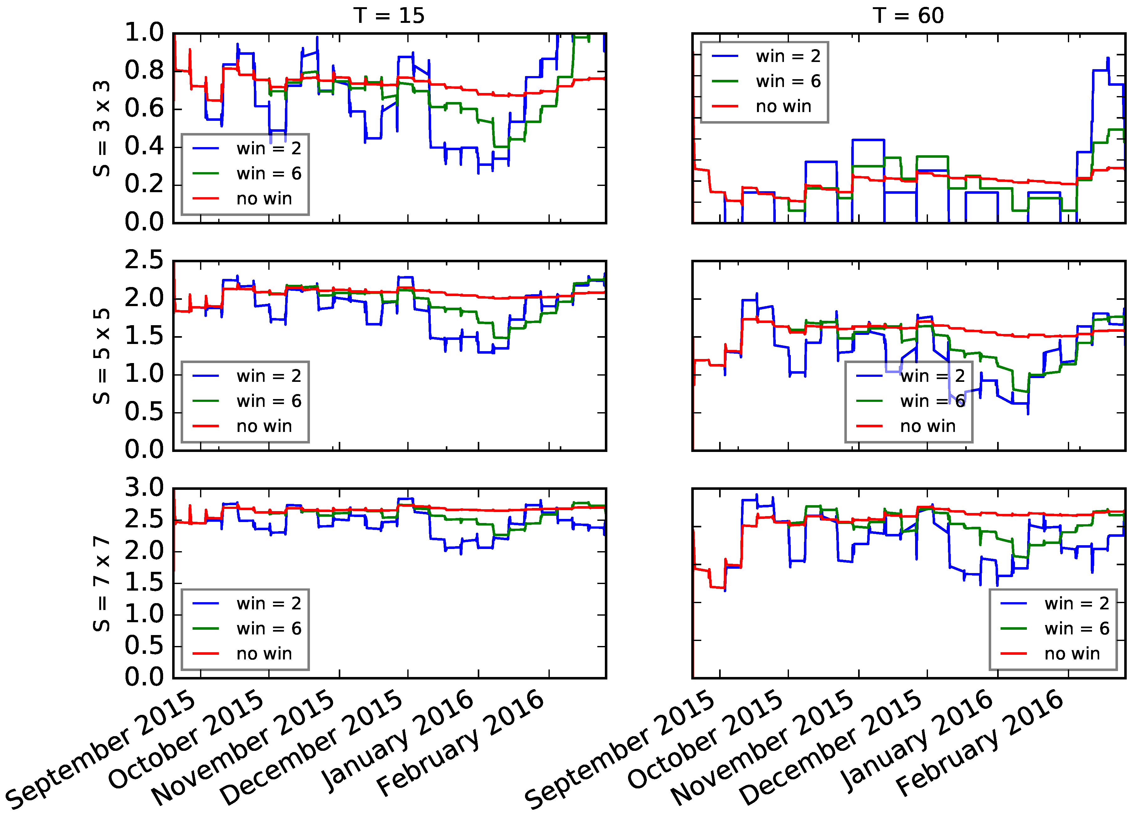
Figure 1 shows some combinations of parameters for one of the days of the week (Thursdays). Other combinations were tested, which are not shown here for brevity.
Figure 1 shows clear differences among all the versions, the main one being the window used for entropy calculation, which allows for changes to be noticed. We can see that with large
T and small
S, we observe too many variations in entropy to allow detecting real anomalies, while large
S flatten the variations too much, not allowing them to be detected. On the other hand, without the window, the entropy flattens when the sequence is sufficiently long, which prevents detecting changes. In conclusion,
T of 15 or 30 min,
S between 5 × 5 and 7 × 7, and
between 4 and 6 weeks seem good.
To decide which combination of parameters
T,
S. and
works best, we applied the following procedure. First, we identified known special days and annotated the specific dates (
Table 1). Next, using the data represented in
Figure 1, we ordered the days regarding the entropy difference with respect to the previous value in descending order (i.e., we ordered the entropy values from the first more likely to reflect an unexpected behavior in the city to the least likely one, and annotated its date), aggregating all days of the week. Then, we checked for each of the ordered days if it corresponded to any of the ones in
Table 1.
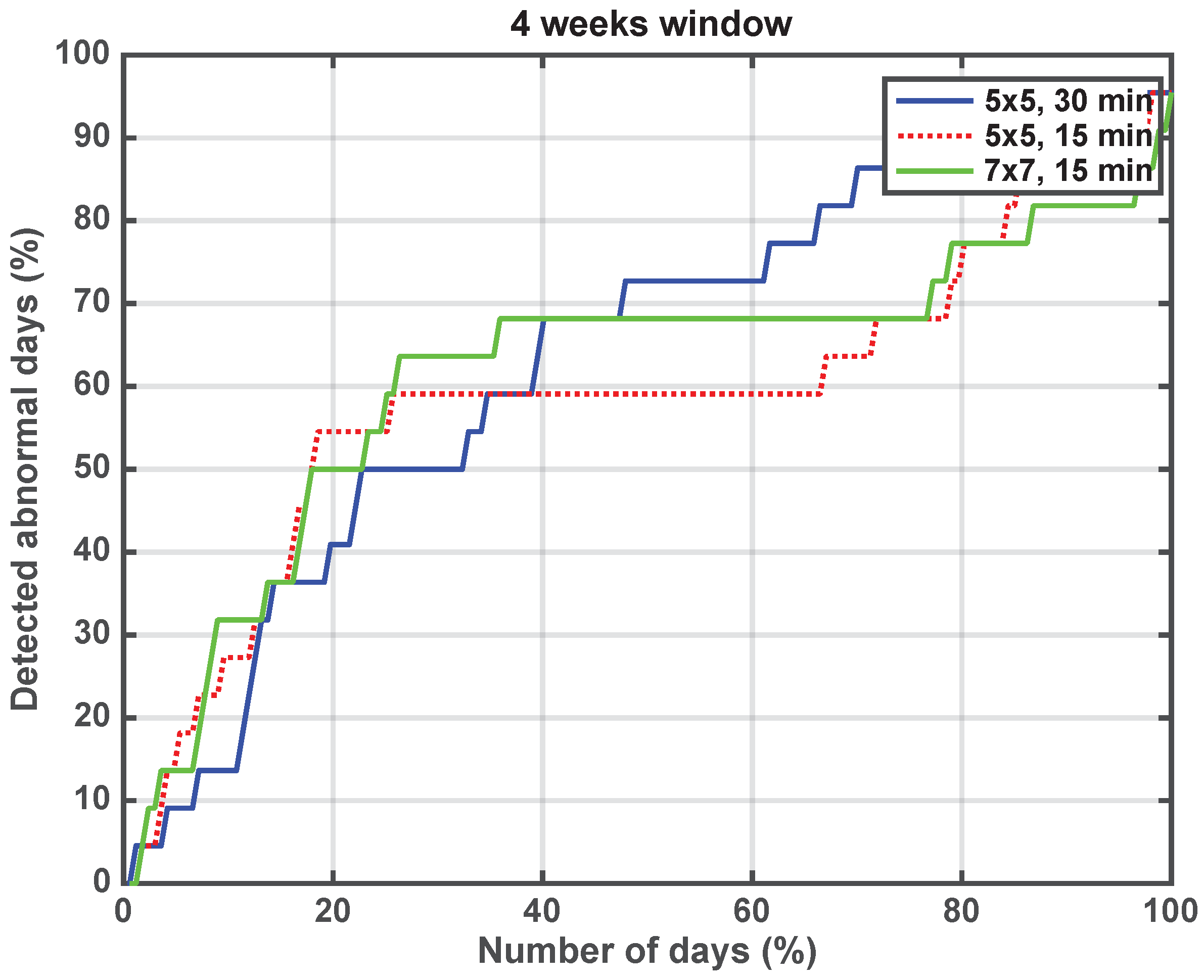
Figure 2 represents the percentage of special days in that table detected when considering the ordered list from top to bottom. For instance, if there are 10 special days out of 100 total days and in the first 10 ordered days, there are 2 special ones, then that means that we can spot 20% of the special days (
y-axis) when considering 10% (
x-axis) of the total number of days. The ideal case would be to spot 100% of special days by analyzing the minimum total days (i.e., all special days are the ones with the highest entropy difference with respect to the previous day).
In
Figure 2, we plot the results of this analysis for different parameter combinations of
T,
S, and
W. With
W = 4 weeks, we can spot up to 55% of special days in the first 20% of the total ordered days. Therefore, in order to identify the highest number possible by considering the least number of total days, a window of 4 weeks is preferable, combined with
min and any grid size (both
S = 5 × 5 and
S = 7 × 7 overlap). Besides these results, something even more interesting came up during the analysis. Taking a look at the steepest changes in entropy (the top values in the ordered list), we further analyzed the contents of the posts and discovered that three of the days at the top of the list corresponded to an unknown event for us: the Comic Con conference, held in New York during 8–11 October (The identification of the cause of the event was made in this work by manually inspecting the posts of that day. In another independent work, we showed how a story detection process can be used (using natural language processing) to find out what is happening in an area [
16]). That discovery ignited the expectations regarding the method proposed as one to capture unexpected behaviors quickly in the city for further analysis using more computationally-expensive techniques to understand exactly what is going on.
5. Validation
In this section, we validate the entropy-based methodology for crowd anomalies detection. First, we compare the abnormal days detected in the data set described in
Section 4.1 using our technique with the ones detected using a different approach. Second, we test the effectiveness of our technique with a different data set.
5.1. Comparison with Results Obtained Using an Alternative Approach
In
Section 4.2, we compared the abnormal days detected using the entropy evolution against a list of special days (mainly holidays) previously identified in
Table 1. In this section, we will compare the consistency of our results with the ones obtained using a different approach. We will first explain the alternative approach considered and then compare the results.
5.1.1. Alternative Approach
In [
12], we defined the criteria to identify moderate and extreme outliers by comparing (i) the clusters obtained applying the clustering algorithm to the real-time data (real-time clustering) and (ii) the clusters in the reference clustering (the behavioral pattern of the city). Both clustering results (reference clustering and real-time clustering) are characterized by a set of clusters, which are specified by two features per cluster: the number of data points and their location.
Note that this approach uses, from the 22 weeks of the data set, 20 weeks as the training set and the other two as a test set. With the training set, we obtain the average location and size of the crowds in the area for each day of the week at each half-hour interval (reference clustering). With the test set, we check the validity of the model (real-time clustering).
Four values or thresholds that define four types of outliers characterize the reference clustering: LMO (Lower Moderate Outlier; LEO (Lower Extreme Outlier); UMO (Upper Moderate Outlier); and UEO (Upper Extreme Outlier). In order to obtain these four thresholds, we adopted the traditional approach [
17,
18] as our starting point. As explained in [
19], an outlier is an observation that lies an abnormal distance from other values. We can display the observations in a box plot with the median and the lower and upper quartiles (defined as the 25th and 75th percentiles). We define the lower quartile as
, the upper quartile as
, and the difference (
) as the interquartile range (
). Then, according to [
17], we define the following values (often called fences):
where
is used for moderate outliers (UMO and LMO) and
for extreme outliers (UEO and LEO). These values of
are the standards in exploratory data analysis ([
17,
19]). However, and in order to avoid negative numbers, we have redefined the lower limits as follows:
This definition reflects that a cluster in the real-time clustering should be considered with an unusually low number of points when it is lower than the
used to obtain the reference clustering, and extremely low when the cluster is empty.
Therefore, identifying an outlier is as simple as comparing the number of data points in a cluster belonging to the real-time clustering with the number of points in the correspondent cluster in the reference cluster. Consequently, if the value is greater than the UEO, we know that the activity should be considered highly abnormal; if the value is greater than the UMO, but lower than the UEO, we know that the activity should be considered as unexpected; if the value is lower than the LEO, we know that the activity should be considered highly abnormal; and finally, if the value is lower than the LMO, but greater than the LEO, the activity should be considered as unexpected.
The essential issue here is to know which is the cluster in the reference cluster that should be used for the previous comparison, i.e., which is the cluster in the reference cluster that fits the cluster under study. In order to determine this important aspect, we have defined the distance between two clusters
and
as follows:
were
is the number of points in the cluster
and
is the distance between a point
, which belongs to cluster
, and the cluster
. Our definition of this distance, between a point and a cluster, is the following one:
i.e., it is the distance between the point
and the closest point that belongs to
.
Finally, a cluster
is considered to fit the reference cluster
if it holds that:
The definitions above allow us to compare both clustering by comparing individually each cluster in the real-time clustering with all the clusters in the reference clustering as follows:
When a cluster in the real-time clustering fits (according to Equation (
5)) a cluster in the reference clustering, the number of points in the former is compared to the four thresholds in order to find out if there is any kind of anomaly.
If more than one cluster in the real-time clustering fits the same cluster in the reference clustering, they will be considered as a unique cluster, i.e., they are merged. Then, the number of points in the merged clusters is compared with the four thresholds in order to find out if there is any kind of anomaly.
All the clusters in the real-time clustering that do not fit any cluster in the reference clustering are considered as Position Outliers (PO), since it entails that we have detected activity in the real-time clustering in areas where it was not expected according to the reference clustering.
If no cluster in the reference clustering fits a cluster in the real-time clustering, we consider that the cluster exists with zero points, and it is considered as a Position Outlier (PO), since there is not activity in a specific area where it is expected according to the reference clustering.
As a result of the comparison between the real-time clustering and the reference clustering, we will have a set of clusters that constitutes the difference clustering. The analysis of this difference clustering allowed us to infer if the activity in the area under study was the expected one or if it shows some outliers [
12].
5.1.2. Ranking of Outliers with the Alternative Approach
The analysis of the difference clustering in [
12] is not enough to obtain an ordered ranking of the detected outliers. This ranking, although it is not essential to detect anomalies, is useful to compare different detection methods, the main objective of the work introduced in this paper.
With this aim, we have established the following set of rules that jointly constitutes a metric that allows us to assign a value or mark, the DoA (Degree of Anomaly), to each cluster in the difference clustering:
if the cluster has a Number of Points (NoP) greater than the LMO and lower than the UMO, the DoA is zero, i.e., the cluster represents an expected or normal behavior.
If the cluster has an NoP greater than the UMO, the DoA is the result of subtracting the UMO from the NoP. This applies for those clusters.
If the cluster has an NoP lower than the LMO, the DoA is the result of subtracting the NoP form the LMO.
If the cluster is a Position Outlier (PO), the DoA is the result of adding its NoP to the maximum DoA calculated for the other clusters in the difference clustering.
The result of adding the obtained values for all the clusters in the difference clustering is the Degree of Anomaly (DoA) of the difference clustering.
5.1.3. Results and Discussion
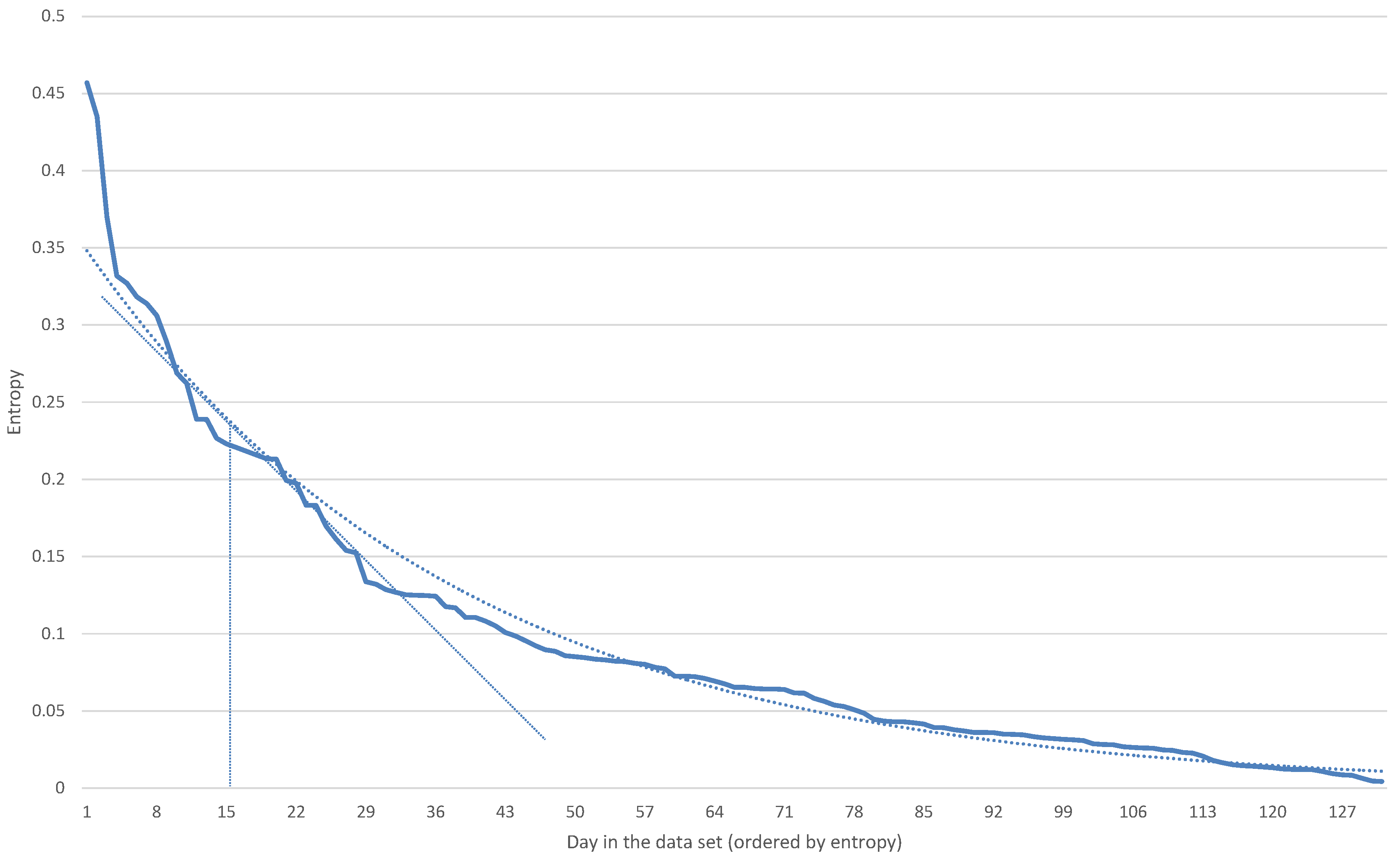
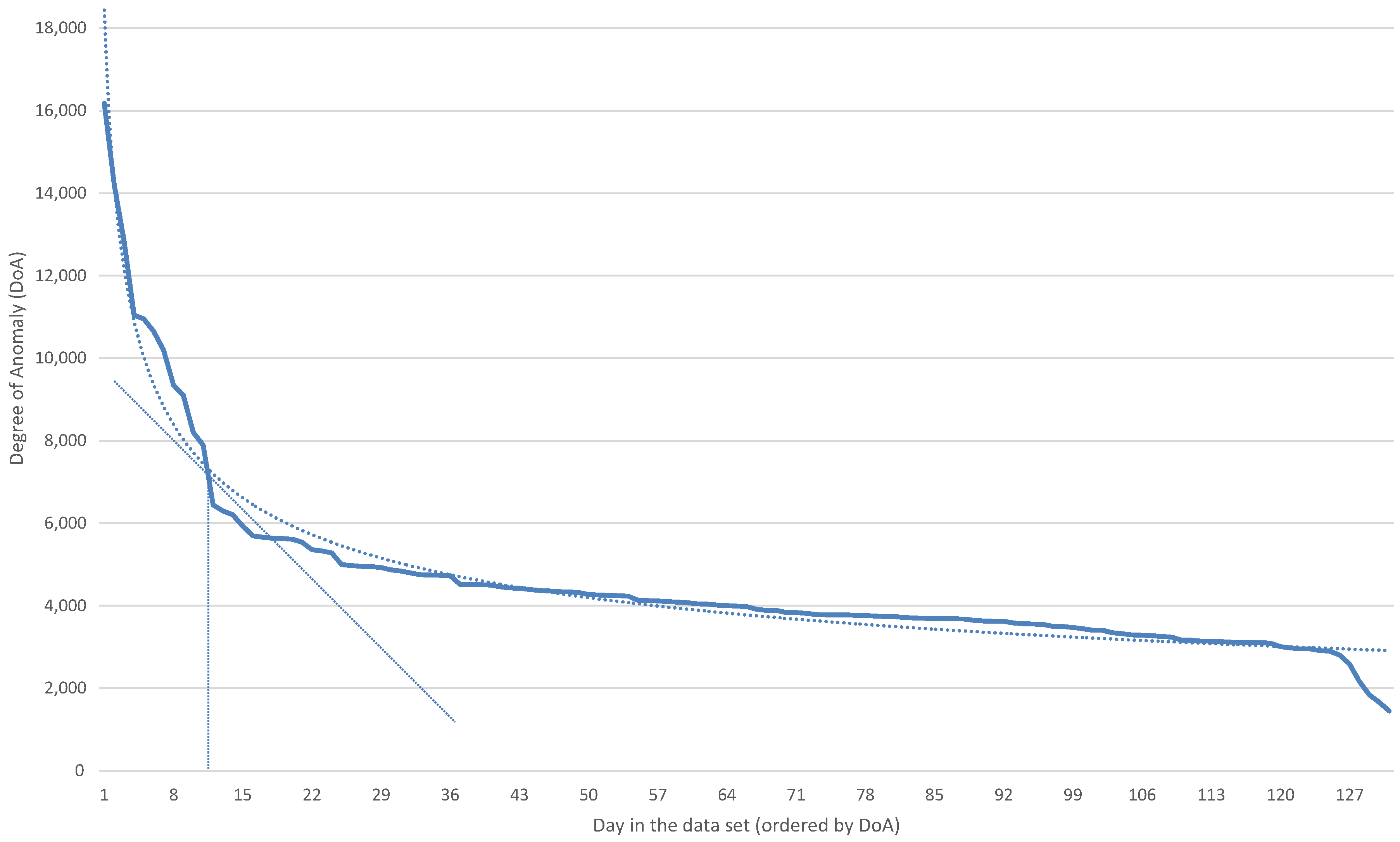
In
Figure 3 and
Figure 4, we show the days in the data set ordered according to entropy-based anomaly detection and to the (DoA) of the difference clustering, respectively.
First, we have to establish a threshold (both in entropy and in DoA) between the days that we consider normal and anomalous. To set this threshold, we considered the point where the slope of the graphs was −1. In
Figure 3 and
Figure 4, we show in dotted lines the trend line, which is exponential in the case of the entropy and follows a power trend line in the case of DoA. We also show the point where the slope of the trend line equals −1. Considering this threshold, the number of abnormal days detected is 16 with the entropy approach and 11 with the DoA approach. Visually examining the graphs, we see that the threshold chosen in the case of DoA corresponds to where there is a rapid rise in the DoA value, while in the case of entropy, we observe a change in trend around Day 27. However, we stick to the thresholds obtained above.
With these thresholds, the list of abnormal days detected with both approaches is shown in
Table 2, together with the position in the rank of each algorithm. We can see that three days appear as anomalous in both algorithms: 10 October 2015, 24 Dedember 2015, and 24 January 2016. One of them corresponds to Christmas Eve, while the two others correspond to events not predicted in
Table 1: the New York Comic Con 2015
https://en.wikipedia.org/wiki/New_York_Comic_Con and the winter storm Jonas
https://en.wikipedia.org/wiki/January_2016_United_States_blizzard. Other potentially abnormal days identified in
Table 2 are not pointed out as such by any of the algorithms, e.g., Columbus Day or Veterans Day.
Examining the list of abnormal days in
Table 2, we observe the following:
The algorithms needed some history to compare past behaviors with present behaviors and to be able to decide if one day was abnormal or not. We have established this initial transient in four weeks. 16 September was the fist day after this transient period, and it was still considered abnormal by the entropy algorithm, not so by the DoA algorithm.
The entropy algorithm better detected consecutive abnormal days, for example long weekends around a holiday, e.g., Thanksgiving, or events lasting several days, e.g., the winter storm Jonas. Note that a travel ban was instituted for New York City for 23–24 January during the storm Jonas and that this was one of the top abnormal days for both algorithms.
On the other hand, the entropy algorithm tended to point out as anomalous wrongly the days following really anomalous days. As it used a four-week window for calculating the entropy, if in the last four weeks, there were several abnormal days, e.g., the Christmas holidays, then the days of the week after Christmas appeared to be different from the previous ones and appeared high in the entropy rank. However, this feature is important for adapting to city changes, e.g., street closures for long-term works.
With these results, we can validate that the entropy approach worked well at detecting abnormal events in the city when compared with an algorithm that was trained with the whole data set but two weeks. The first advantage of the entropy-based outlier detection is that no previous patterns for training are needed, since it is continuously learning from the location of the posts obtained from Instagram. After an initial transient period of four weeks, anomalous data increase the entropy values and abnormal events start to be detected. The second advantage is that the entropy levels are continuously adapted as long as new geolocated data are extracted from social media. New patterns are learned. and older patterns are forgotten, adapting to the evolution of the city.
Regarding the computational cost of the entropy algorithm, it is very simple and can be implemented in real time with low resource consumption. Since we used the windowed version of the entropy,
, the computation cost of the entropy depended on the number of symbols in the sequence,
, and the cardinality of the alphabet
(i.e., the number of possible different symbols in our distribution). In our case, the cardinality of the alphabet was the number of cells in the grid in which we divided the city. Assuming a grid of
cells,
. Both quantities are constant and small, and Equation (
3) can be computed in a fixed, short time.
All the results presented so far were obtained using the New York data set. We will check next if the algorithm works well with the same parameters used before in a very different data set.
5.2. Validation with a Different Data Set
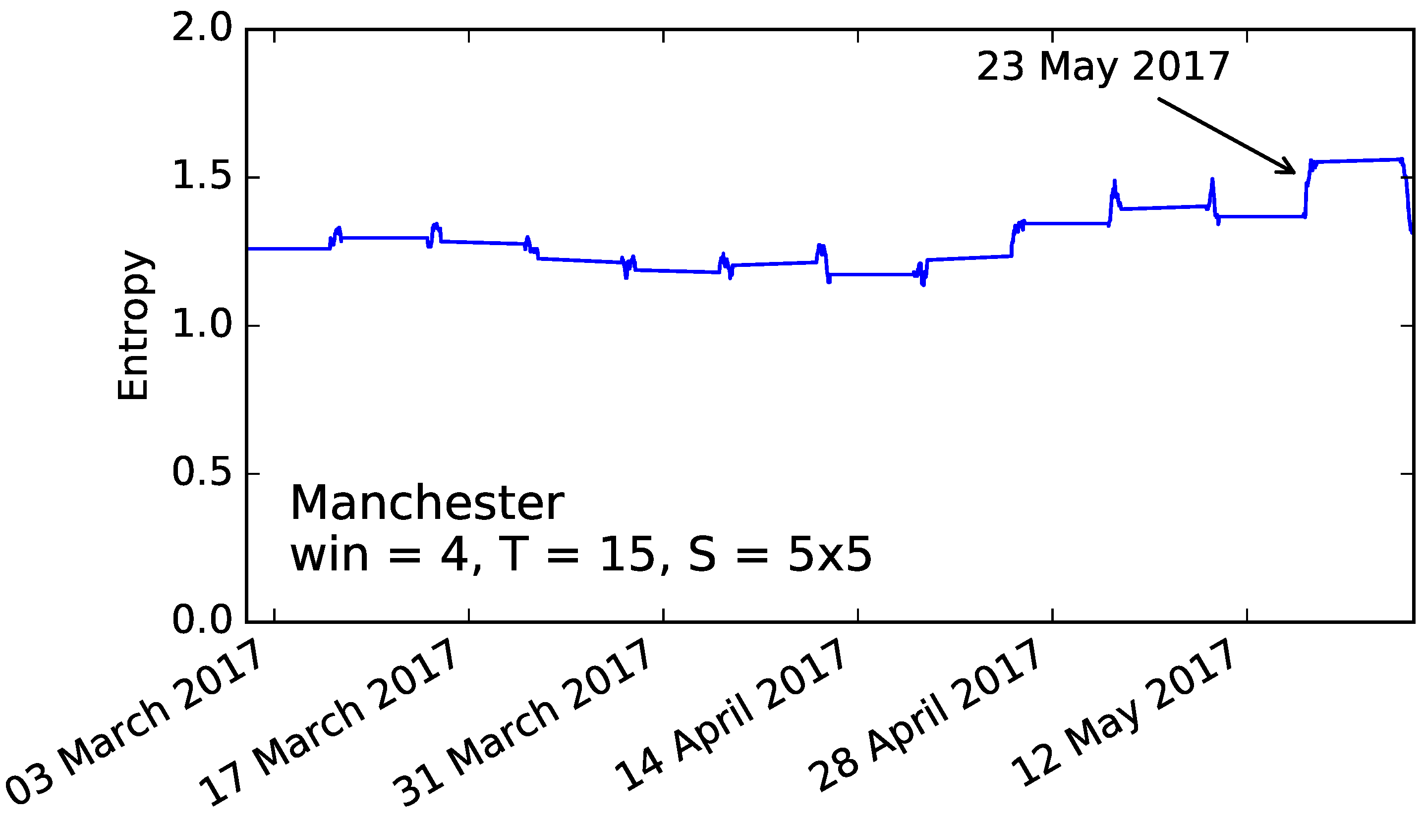
To validate the selected parameters, we applied them to another data set obtained in a city with different characteristics. We collected geolocated Instagram posts in Manchester for four months.
Figure 5 shows the entropy evolution of Tuesdays using the same parameters chosen for the New York data set in
Section 4.2:
,
,
S = 5 × 5. We can observe a remarkable increase in entropy on 23 May, following the terrorist attack on the evening of 22 May 2017
https://en.wikipedia.org/wiki/Manchester_Arena_bombing. This was by far the day with the highest entropy increase in all the data set, with an increment of 0.22.
6. Limitations
One of the limitations of using Instagram or any other social network to detect anomalous events is that it is very sensitive to changes in API policies. At the time we carried out the New York data capture campaign (end of 2015 and beginning of 2016), the Instagram API media/search endpoint allowed recovering data from any moment in the past, between two timestamps (you can see the API at the time of our data capture campaign at the Internet Archive:
http://web.archive.org/web/20150531210319/https://instagram.com/developer/endpoints/media/), so our data set could be re-extracted later by anyone (for example, if she/he would like to reproduce our study). This is not possible anymore. Besides, since June 2016, for privacy reasons, the media/search endpoint in Sandbox mode was limited to return just the media you uploaded from that location. To have access to the public content published by others, you need to submit your application to Instagram for approval for the Live mode. This was not required when we made the New York capture campaign.
Another limitation of our approach is about how the Instagram API media/search endpoint provides geolocated posts. The location of the post was obtained from the latitude and longitude where the photo was taken (provided by the device). However, Instagram does not provide public information about the percentage of Instagram posts that contain geolocation. According to the survey study in [
20], 30% of the respondents said they geotag all posts, and 30% said they never geotag posts; however, 60% claimed to geotag some of their posts, and about 10% claimed to geotag half or more of their posts. Although an accurate percentage cannot be provided without the official data from Instagram, taking into consideration the information in [
21], it could be claimed that geotagged posts increase engagement up to 79%. Additionally, we can argue that Instagram is one of the most geolocated social networks, since the percentage of geolocated posts in Twitter was just 1% in 2014 [
22], the same year as the study in [
21].
A possible question is whether there may be events of interest that may not be detected using Instagram because they were not attractive to their users. In this work, we are interested in detecting unusual events such as emergencies. In [
23], the authors presented the results of a study on citizens’ perception of social media in emergencies conducted in Germany. The study highlighted that around 24% of people have used social media during an emergency to share information. When asked about what types of information they share, 37% of the times they share the location and some photo or video. According to this study, we expect emergency events to be identifiable on Instagram, as we have found in the two study cases (New York and Manchester) presented in this paper.
Finally, some recent papers ([
24,
25]) studied content bias in crowd-sourced geographic information in OpenStreetMap, depending on the country and the culture. Another work presented a similar study during disasters ([
26]). It is difficult to know if there are deviations of this nature in the data we obtained from Instagram. We do not know the information that could be relevant to study these biases, such as age, nationality, cultural level, etc., of post authors. However, we believe that our use of social networks (specifically Instagram) differs from that of OpenStreetMap in these works in two important aspects. First, the posts we obtained were generated in a very limited are (radius of 5 km), so we did not expect great differences in demographic and social characteristics of the post authors. Second, in OpenStreetMap, the geographic information is explicitly crowd-sourced by the users (they make an explicit action to send the information), while in our work, we collected the geographic information from Instagram without the users being aware that they were participating in this process. We believe that this unnoticed collection process protects against the biases that occur when the user explicitly sends the information. Anyway, these aspects remain open and need further investigation.
7. Conclusions
This paper proposes a new entropy-based methodology for early detection of anomalies in urban areas that exploits the location data of the posts published on LBSNs. The proposal uses a centroid as the single geographic point summarizing the pulse of the city, the location of which is tracked to detect changes in its entropy evolution. Although more than one point could be used to represent the citizens’ movement all around the area under study, working only with one centroid allows obtaining quick and sound results.
From the time sequence of centroids that summarize the pulse of the city, just the last W weeks were considered, and the centroids were discretized into an grid. We studied different values of the parameters, and we found the best results with and . We then used the entropy of the discretized sequence of centroid locations in the last W weeks to detect anomalies.
The main advantage of our algorithm is that there is no training phase, so the algorithm starts detecting abnormal days from the beginning, with good results after the first W weeks. Another advantage of our approach is that it can adapt to changes in the dynamics of the city, since at the same time it learns new patterns from current posts, it forgets old (more than W weeks old) patterns. The algorithm is simple and fast, so it can be executed in real time with low resource consumption.
The validation was done with seven months of geolocated data from Instagram posts published in NYC. Apart from correctly identifying up to 55% of expected abnormal days (Christmas, holidays, etc.), the solution was able to discover events we were not aware of, where an unusual pattern was clearly detected by our proposed methodology, and further analysis of the content of the posts uncovered the reason. The parameters selected were also validated with other data set, from Manchester, where the effects of a terrorist attack in the entropy of the crowd dynamics can be observed.
We are currently working on two lines: on the one hand, extending the algorithm to work with more than one centroid (two, three) representing the movement of the whole population in the city; on the other hand, the analysis presented in this paper shows the changes (of entropy or DoA) at a day level. This analysis can be presented at shorter intervals (every 15 or 30 min) to show sudden changes in the city as they occur.
In this work, we have considered aggregation of Instagram posts at fixed time intervals (15, 30, and 60 min). As future work, other forms of aggregation of posts can be investigated. Posts could be aggregated in variable length time intervals, aggregating a constant number of posts (e.g., 200 post) per time interval, so that the time intervals would be shorter or larger depending on the activity (the number of posts) on Instagram. Surely, this could help detect the events that cause a large number of posts faster.


