A Novel Detection Technique for a Chipless RFID System Using Quantile Regression


1
Department of Information Engineering and Computer Science, University of Trento, 38100 Trento, Italy
2
Department of Electrical Engineering, Indian Institute of Technology Hyderabad, Telangana 502285, India
3
Department of Electronics and Communication Engineering, Amrita Vishwa Vidyapeetham, Amritapuri 690546, India
*
Author to whom correspondence should be addressed.
Electronics 2018, 7(12), 409; https://doi.org/10.3390/electronics7120409
Submission received: 11 November 2018
/
Revised: 29 November 2018
/
Accepted: 3 December 2018
/
Published: 8 December 2018
(This article belongs to the Special Issue Unconventional RFID Systems)
Abstract
:This work presents a novel approach for improving the detection capabilities of a chipless Radio Frequency Identification (RFID) system based on quantile regression. The main drawback of chipless RFID systems is the limited response of the tags due to the low-quality factor of the resonators, used to encode the information in the tag. The detection becomes very challenging especially for real-time data when noise is present. This work proposes the use of quantile regression to enhance the system performance. A chipless RFID system prototype has been fabricated (as a proof of concept) and experimentally assessed. The obtained results are quite satisfactory in the potentialities of the proposed methodology.
1. Introduction
Radio Frequency Identification (RFID) has been one of the most influential inventions in the last decades. Over these years, this technology has become mature enough to be used in various applications, such as health monitoring, supermarket food and goods tracking systems, libraries in book tracking systems, environmental sensing [1], and for Internet of Things (IoT) applications. The current research as regards chipless RFID focuses on cost and a compactness [2]. The RFID technique that eliminates the use of the chip is called “chipless RFID” [3]. The chipless RFID techniques can be divided into two groups based on the encoding mechanisms: time-domain (TD) or frequency-domain (FD), as in Reference [4]. In order to overcome the issue of cost, different types of approaches have been taken. In References [5,6], high-density compact chipless RFID tags for item-level tagging and switch controlled RFID employing a external laser light source are presented, respectively. Whereas, References [7,8] focus on low manufacturing cost, compactness, flexibility, and efficient bandwidth utilization for IoT based sensing applications. In Reference [3,4,9,10,11,12,13,14,15,16,17,18,19,20], various shapes of resonators are proposed to increase the compactness and flexibility. Nevertheless, some researchers [21,22,23,24,25,26,27,28] have discussed various ways to increase the range of the RFID. Wherein, References [4,14] have also proposed a way to increase the data capacity and coding capacity of RFID tag, respectively. In Reference [11], a novel approach for a chipless RFID sensor tag design integrating dipole resonators as the ID encoders and a circular microstrip patch antenna (CMPA) resonator as the crack sensor for metal crack detection are proposed. In detection, reading, and identification of the tag, various studies have been presented [29,30,31,32]. In Reference [33], the resonances in spectral encoded chipless RFIDs were performed. This method uses the second-order derivative of the phase of the signal instead of its amplitude and does not require a reference signal. However, research from Reference [34] draws attention towards the security of IoT devices against the attacks such as Denial of Service (DoS), tag/reader anonymity, and tag impersonation.
In this work, an improvement to the detection capabilities of the chipless RFID system based on quantile regression method is proposed. The work is organized as follows. Section 2 describes the chipless RFID system and provides guidelines for the design of a chipless tag on spiral resonators. In Section 3, the quantile regression model is explained in detail. Section 4 is devoted to the numerical assessment. Later in Section 5, an experimental assessment is carried out with an experimental chipless RFID system.
An implemented measurement campaign was performed considering different tag considering different tag configurations by using copper tap tape. The tag was placed at 10 cm from the reader, the power of the transmitter was −12 dBm. However, it is possible to increase the operative range by increasing the power of the generator or antenna gain. Moreover, the noise was added (with the resistive loads). The measured insertion losses collected with the SA124B receiver were processed with the quantile regression tool in order to correctly identify the tag’s bits. An accuracy of 95% was obtained with the experimental data demonstrating the accuracy of the quantile post-processing tool of the proposed system. Finally, Section 6 reports the conclusions and some remarks on future work.
2. System Description
In this section, the description of a chipless RFID system is presented. Figure 1 shows the schematic of the system. With reference to Figure 1, the reader contains a sweep signal generator, a power splitter, a circulator, a mixer, a low pass filter, and an analog to digital converter. The mixer down-converts the detected RF signal, and a low pass filter removes the high-frequency components. This mixer with the lowpass filter implements a homodyne detector mandatory to retrieve the signal correctly. A tag section comprises two main elements, spiral resonators, and two antennas. Here, we have used multiple resonators in our experiment. As shown in Figure 1, all the resonators are in cascade form, and they are connected with circular polarized antennas. The distance between the reader and tag is defined as the operative range at which information is correctly retrieved from the tag by the reader. When the RF signal impinges on the receiving (Rx) tag antenna and propagates further towards the resonating circuit, cascaded spiral resonators produce phase frequency jumps at particular frequencies of the spectrum, which encode the data bits. Later, when the signal has been passed through the resonating cascade resonators, the unique spectral signature of the tag is transmitted back by means of the transmitter antenna (Tx) tag. This re-transmitted encoded signal is detected and presented to the reader. This digital signal is obtained on a computer system for the post-processing. As a post-processor, we used a quantile regressor. A detailed description of the quantile model is described later in the next sections.
Tag Description
This section provides the guidelines for the design of chipless tags based on spiral resonators. In addition, The tag structure is given in Figure 2, it consists of the main microstrip feeding line and a set of spiral resonators [35], which encode the data into bits.
Spiral resonators provide better performance on thin laminates because the resonators are fabricated in microstrip or coplanar waveguide technology. Spiral resonators are a better alternative to the simple stub resonator, since they provide a satisfactory quality factor (Q) with respect to a simple stub resonator. As shown in Figure 2, the resonators are coupled to a microstrip line and modeled using distributed elements. The design parameters and the layout calculation of the microstrip spiral resonator are defined as follows.
The width of the microstrip line is , is the gap between the resonator and feeding line, and the width of the spiral conductor is . The separation between the spiral conductors is , the length and width of the spiral resonator is . and are the distance between the resonator and ports. The total length has been represented by , is number of the spiral resonators sides, is the wavelength, is the light velocity, and is the permittivity of the dielectric substrate, respectively. A small gap between the feeding line is used for activating the resonators [36].
The total length of the spiral resonator has been estimated using Equation (1). The length of the resonator at the resonance wavelength can be calculated using the following Equations (2) and (3), respectively. It is worth noticing that Equation (2) provides only a rough approximation of the resonator length . Please note that the above formulas are approximated and a tuning phase frequency aimed at refining the resonator geometrical parameters is mandatory to obtain an accurate resonance.
3. Quantile Regression for the Peak Detection
This section is aimed at explaining the quantile regression model used to improve the detection capabilities of the chipless RFID system. Quantile regression, which was introduced by Koenker and Bassett (1978) [37], seeks the estimation of conditional quantile functions. As given in Reference [38], this model quantiles the conditional distribution of a response variable and expressed as a functions of independent variables. Other linear regression models have the relationship between one or more independent variables and the conditional mean of a response variable; in contrast, quantile regression intends to find out the influence of independent variable(s) on a response variable in terms of range variation and conditional distribution.
Therefore, quantile regression has the capacity to provide a whole picture of distribution characteristics and a more complete statistical analysis [39]. In addition, quantile regression is more robust to outliers relative to least squares regression when estimating parameters [40]. Furthermore, the quantile regression model does not require any dataset for the training of a model like in the classification model. The main difference between quantile regression with linear and other regression models is that a quantile regression does not require any specific distribution like the others. In the past decade, quantile regression has become very useful in comprehensive statistical analysis methods applied in various fields such as economics, medicine, environmental science, survival analysis, botany, and zoology in the form of linear or non-linear models [41].
Here, the quantile regression model has been adapted to predict the frequency shift and amplitude variations of peaks of the resonators, which encode the data. A quantile regression is commonly applied to solve parametric, non-parametric, and semi-parametric regression problems in statistics and economics [42]. Quantile regression turns out to be particularly useful when the distribution formation cannot be defined and the other regression models are not applicable or require too much customization. It is worth noticing that depending on the problem at hand, there are different regression models characterized by unique structure and responses depending on a measurement scale and distribution. This is the situation of chipless RFID system where the peaks, which represent the information, could present a frequency shift and different depths values due to noise, material tolerances, and fabrication defects. The peak depth and frequency shift are difficult to predict and model. As described in Figure 1, when the RF signal is transmitted back with the unique spectral signature, the signal is recovered at the reader. In particular, the encoded data can be observed in the insertion loss y signal. The behavior of the y signal shows that at a particular frequency, the signal gives a phase frequency jump which is recorded as peaks and represents the encoded bit value. In post-processing, the phase frequency, observed in the signal behavior, is detected, and the decoded data bits from the signal are retrieved by means of the quantile regression model. The mathematical model for the quantile has been described as follows.
The is the detected signal at the reader signal and are the frequencies at which resonators perform, where represents the number of samples. The signal collected by the Rx antenna shows that the y signal does not follow any particular distribution form. Therefore, in order to detect the peak, we have applied quantile regression on the given data as a post-processor. As described earlier, the quantile method is very useful when the signals distribution function is unknown. The theoretical quantiles of a random variable are commonly and implicitly defined by its probability values. In which, through its observed probability values it calculates the weighting function. The weighting function commonly gives the quantile of the given data [42].
As per the model shown in references [42,43], the mean , unconditional mean and the variance of the signal y have been calculated. The knowledge of mean value provide the unconditional mean and probability of the signal y at a sample of the signal y. Equation (4) is the unconditional mean for all . It provides the mean value at a particular sample of signal y. The following weight function (5) calculates the weight of the function using the unconditional mean and the probability of the signal . Equation (5) provides the peak of the signal as shown in numerical assessment. However, the above mathematical model works only in ideal condition where there is no noise. For all the samples, the weight of the function detects the location of the peak at the given frequency range but in the case of frequency shift, Equation (5) fails. In addition, when we considered the noise, the noise produces the frequency and amplitude shift as we have shown in numerical assessment.
In order to overcome the issue of the frequency and amplitude shift, and the noise, we implemented a new weighting function (6). The advantage of this function is that instead of calculating a quantile of the whole signal , this function calculates the quantile for the conditional mean value for a given frequency step size , , where and are the lower and the higher frequency values of the signal y. We have calculated the bandwidth of the given signal y, which also represents the frequency range of the signal y. Equations (7) and (8) have been used to calculate the percentage quantile range value (starting from 10% to 100%) for each frequency step size . In References (7) and (8), a frequency step size is represented by which gives the quantile percentage value. In Equation (7), the value of decides the range of the and by giving length of . For simplification, we have chosen the quantile percentage value as so that the length of is .
Moreover, for all the possible values of in Equations (7) and (8), the weight of the function is calculated from Equation (6). In Equation (6), instead of the probability we have changed the parameter to the signal . The Equation (6) estimates the peak more accurately than the Equation (5) because Equations (7) and (8) work like a moving window for the considered frequency range. The movement of the windows is defined by the frequency step size . Here, has been verified over all the possible range of . The possible range value of a decides the window size. Equation (6) detects the frequency shift and phase magnitude shift of the signal for a smaller window size as shown in the numerical assessment. However, in an experimental assessment, we have noticed that Equation (6) detects false peaks for the smaller window size. Further explanation on this matter is given in the Section of experimental validation. The experimental assessment proved that even in a real-time environment where noise is high, our proposed algorithm is able to detect the peak. Equations (5)–(8) provide all the information needed to calculate the peak at a given frequency range. It is worth noticing that after the proposed weighting function, we get satisfactory performance and accuracy of peak detection.
4. Numerical Assessment
This section is aimed at numerically assessing the proposed methodology. In particular, a tag, composed of five resonators, able to encode 5-bit data with combinations is considered. The tag structure was modeled and simulated by means of a commercial software namely ADS2017 by Keysight Technologies (Keysight Technologies Inc., Santa Rosa, CA, USA). The tag was designed to operate in the Wi-Fi frequency band at the central frequency of 2.45 GHz. The considered dielectric substrate was ARLON25N, , thickness t = 0.8 mm, . The geometrical details of the considered five resonators are reported in Table 1 with the correspondent resonating frequencies. Concerning the other geometrical parameters, they are = 1.61 mm (microstrip width) and = 0.2 mm (the coupling gap between microstrip and resonators). To simulate the different tag combinations, a given resonator can be short-circuited by means of a vertical metallic slab. In particular, a short-circuited resonator represents a “0”, while a resonator without a metallic slab encode a “1”. For almost all tag configurations, a simulation with ADS2017 was performed in order to simulate the signal received by the reader in the frequency range from 2.4 GHz to 3 GHz. Figure 3 represents the simulated received 5-bit signal at the reader for a tag configuration of 11111 (all the resonators activated). It is worth noticing that we have used a 5-bit tag configuration only to provide a proof of concept system and to numerically and experimentally assess it. Theoretically, the quantile regression method can be applied to detect data of any length and certainly longer than 5 bits. As it can be noticed from the data reported in Figure 3, the peaks of resonance which identify the bit “1” are clearly evident even if not so deep. For all the numerical experiments, the post-processing tool based on the quantile regressor (implemented in MATLAB) was applied to the signal obtained with the ADS.
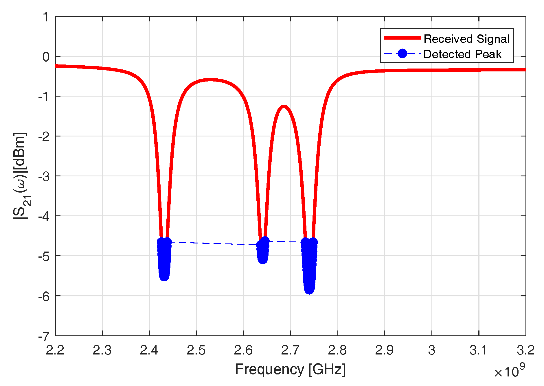
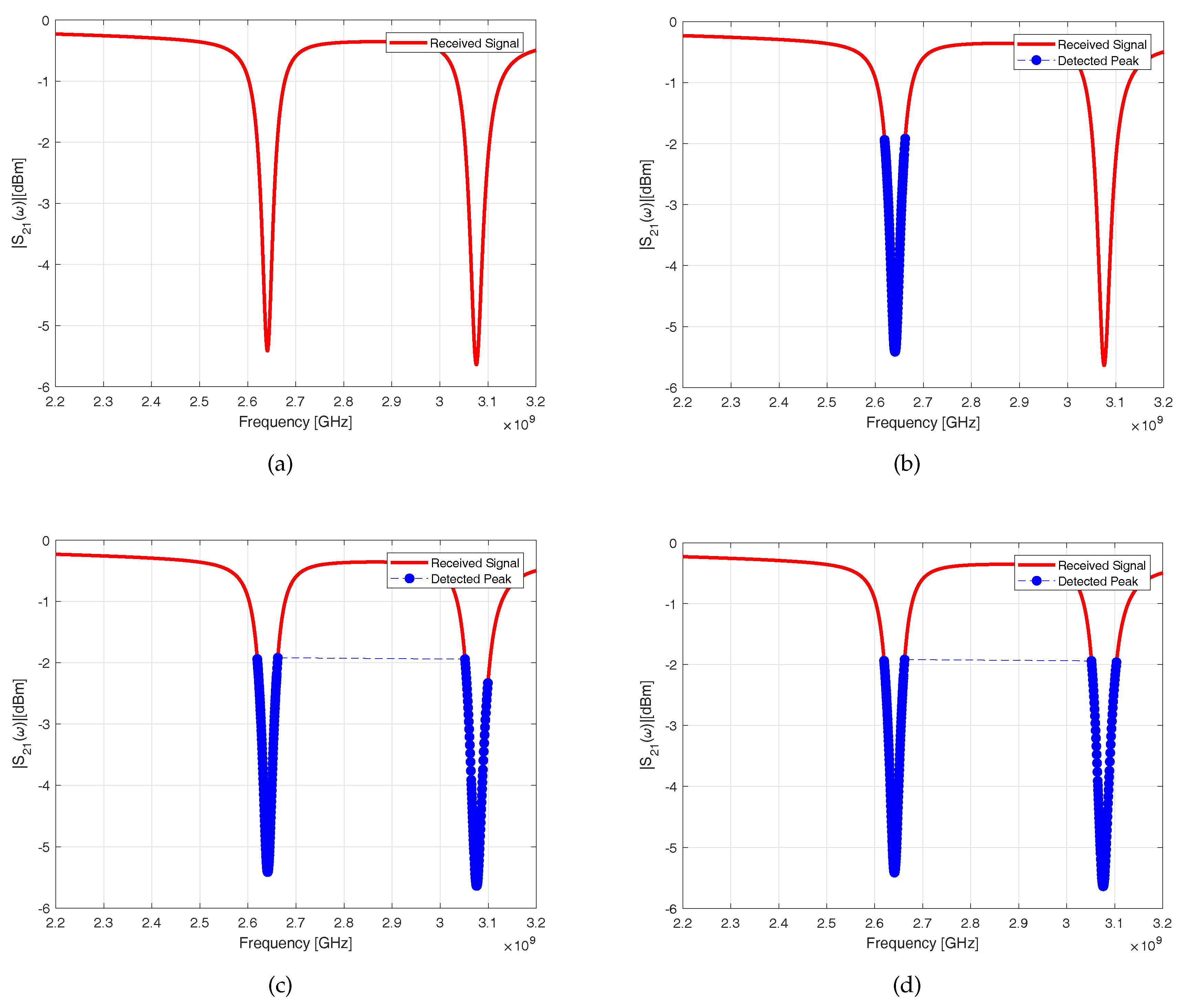
Figure 4 reports the peak detection obtained with the regression method reported in Section 3 for the a tag characterized by three active resonators (tag configuration “10110”). The data have been numerically generated with a peak depth and frequency shift variations of 10%. As it can be noticed from the data in Figure 4, the peaks are correctly identified, the blue dots identify the frequency range of each resonator. The process of peak identification obtained by considering the quantile regression reported in Section 3 which consider the new weighting function (6) is reported in Figure 5. In addition, the data reported in Figure 5 were numerically generated and corrupted by random amplitude and frequency range variations for each peak. The received signal is reported in Figure 5a. Figure 5b–d shows the detection of peaks located between 2.4–2.5 GHz (b), 2.6–2.7 GHz (c), and 3.1–3.2 GHz (d), respectively. The data reported in Figure 6 refer to the tag configuration 00101, where two resonators are active and three short-circuited. Furthermore, in this case, the data were numerically generated, Figure 6a reports the simulated data received at the reader and corrupted with a random error on the peak amplitude depth of ±3 dB and a random frequency shift error of of the active resonators. Additionally, in this experiment, all the peaks (corresponding to bit “1” in the tag) are correctly identified. In particular, Figure 6b–d clearly show the different identification steps of the quantile regressor. To better simulate realistic scenarios, different kinds of noise scenario was added to the obtained synthesized signal . In particular, a strong additive white Gaussian noise (AWGN) as well as random frequency shifts and amplitude peak changes were added to corrupt the simulated data. In particular, Figure 7 reports an example of data corrupted both by 10dB AWGN noise, a random amplitude variation, and a frequency shift of 10%. Furthermore, in presence of a high noise level, the quantile regressor is able to identify the peaks with a high degrees of accuracy. Particularly, Figure 8b–d clearly show the different identification steps of the quantile regressor. It is worth noticing that only a selected set of results has been reported in this section to demonstrate the potentialities of the method. The quantile regressor was tested on several combinations and considering different scenarios with different noise levels, frequency shifts, and peak depth variations. Notably, the numerical assessment was performed by considering more than 200 different configurations obtained by adding noise to the original sequences; the method based on quantile regressor demonstrated its potentialities showing a success rate of about .
5. Experimental Validation
In order to assess the capabilities of the proposed system, an experimental system prototype (acting as proof of concept) with different tags was fabricated and assessed. The reader is a monostatic continuous wave radar (CW) composed of a sweep signal generator (TG124A, 100 KHz–12.5 GHz from Signal Hound USB-TG124A, La Center, WA, USA), a circulator (RE83CR1004, 2 GHz–4 GHz from Pasternack, Huntington, CA, USA), a broadband circular polarized antenna [44]. The receiver is a SA124B spectrum analyzer (100 KHz–12.5 GHz from Signal Hound, La Center, WA, USA). The schema of the reader is reported in Figure 1. Concerning the tags, they are fabricated with two kind of dielectric materials, the ARLON25 (h = 0.8 mm, = 3.28, tan = 0.001) and FR4 (h = 1.0 mm, = 4.2, tan = 0.001). In particular, tags with five spiral resonators tuned considering Table 1 were considered. In order to compare the experimental measurements with the simulations reported in Section 4, the resonators were excited by means of a microstrip line, and fed by the two antennas (a Tx and Rx one) connected to the tag using two sub-miniature type A (SMA) coaxial connectors. To obtain one of the different tag combinations, a copper tape was used to short-circuit the resonators (and exclude them) to obtain “0”. Figure 9 reports a photo of the tag prototype (a proof of concept) with five resonators and the two broad band circularly polarized antennas connected. To increase the number of possible combinations and further increase perturbation/noise in the measured data set , different surface mount device (SMD) resistive loads were soldered at the end of spiral resonators. The resistive loads are usually inserted to provide sensing capability to the chipless tag. In this work, the resistive loads were used to simulate frequency shifts and resonating amplitude variations. An example of the effects of the resistive loads on the resonator response is reported in Figure 10. The loads were connected to the last resonator designed to resonate at 3 GHz as indicated in Table 1. The use of resistive loads permitted us to increase the experimental data set, their effects being quite evident as shown in Figure 10.
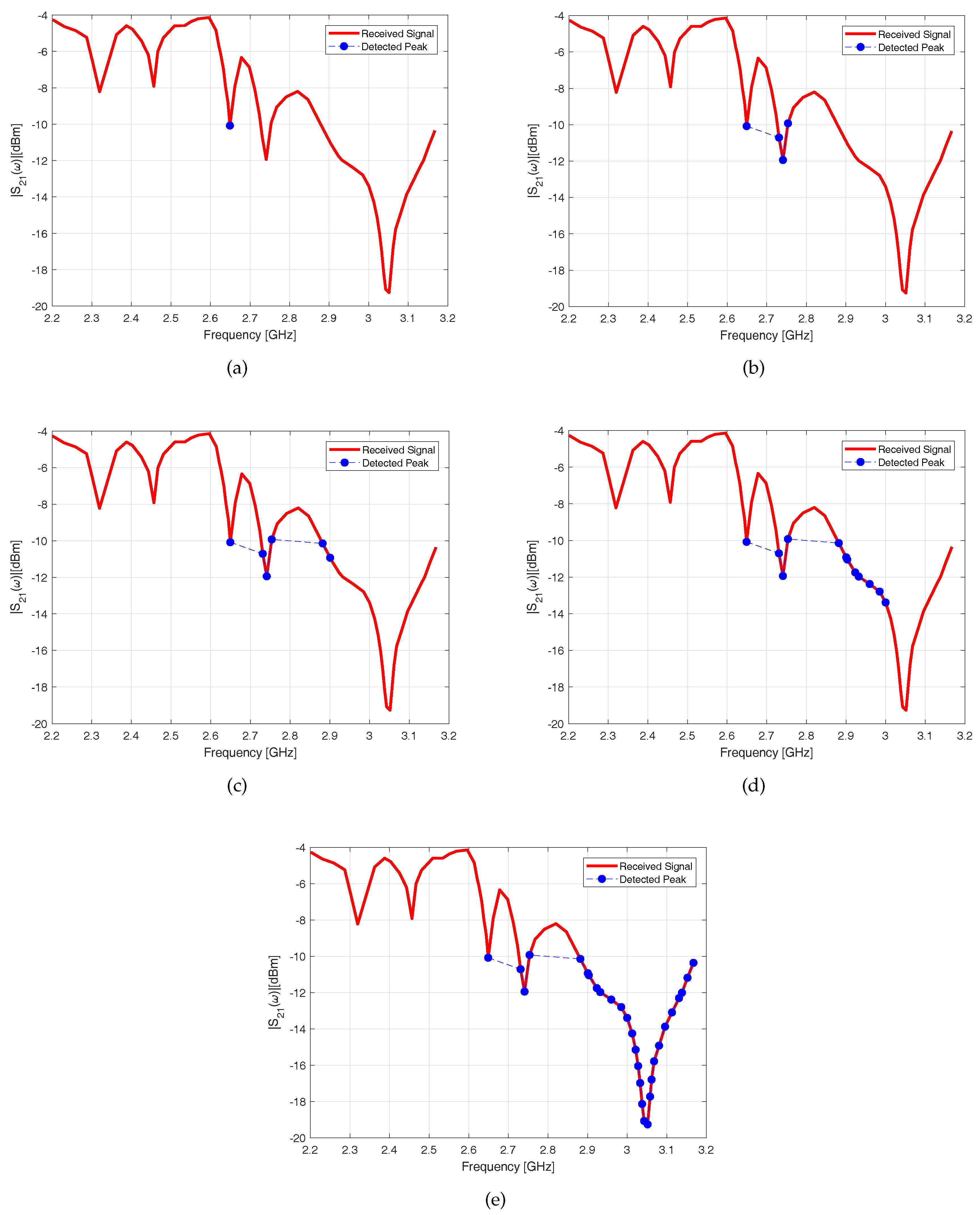
The prototype demonstrator is, shown in Figure 9, was tested considering different tag configurations. A copper tape was used to insert a short circuit on a given resonator and to obtain a “0”. Figure 11a reports the experimental data obtained for the tag configuration 11110, the last resonator was short circuited by means of a small slab of copper tape. The different steps of the quantile regressor post-processing process are reported in Figure 11b–e, respectively. As can be seen from the data reported in Figure 11, the peaks which encode a “1” are correctly detected despite the noise level and the different amplitude level of the first two resonators with respect to the others. As well as for the numerical validation, the experimental assessment section presents only a selected set of results. For the sake of completeness, experiments with different tag configurations were carried out. In addition, with experimental data, the quantile regressor method demonstrated its potential showing a success rate of about . The number of tag configurations was improved by loading the five resonators with resistive loads (soldering surface mounted SMD components). Additionally, in this case, the number of tag configurations was extended from to 200. The last experiment reveals the limitations of the proposed methodology based on the quantile regressor method. Problems arise when the peak depth is too perturbed. A typical scenario is reported in Figure 12a, which shows the signal retrieved at the reader for a tag with all five resonators activated (tag configuration 11111). As can be seen, the quantile regressor procedure is able to correctly identify only the last three peaks (Figure 12a–e). The first two resonances were not correctly identified. This is certainly due to the high difference between the peak depths. It was observed that when the peak amplitude difference between the resonances is greater than 10 dB, some peaks can be lost. The scenario reported in Figure 12 presents a depth difference of about 11 dB between the first two resonances, located in the frequency range from 2.2 and 2.5 GHz, and the last peak located between 3.0 and 3.1 GHz. This condition occurs only when the resonators present too much difference in quality factor. In the last experiment, a high peak perturbation was deliberately introduced by using a resistive load = 1500 on the last resonator to assess the robustness of the proposed methodology.
6. Conclusions
In this work, a method for improving the detection capabilities or a chipless RFID system is proposed. The method is based on a quantile regression algorithm able to correctly retrieve the tag information under different noise conditions. The method was numerically and experimentally assessed by means of tag prototype (a tag demonstrator) composed of five spiral resonators. The obtained results are quite promising. However, in the experimental assessment we observed that the resonators quality factor has to be the same as regards the design of the resonator. The difference in quality factor affects the insertion loss which produces the phase magnitude and frequency shift. This difference also produces false peak detection in noisy environments. In our future work, we will try improve our method in order to detect peaks in noisy environments and in scenarios with resonators of different quality factors.
Author Contributions
M.D., S.K.M. and A.K. conceived and designed the idea and the experiments; M.M. developed the quantile code, performed the experiments and analyzed the data. M.D., S.K.M. and A.K. wrote the paper.
Funding
This research received no external funding.
Conflicts of Interest
The author declare no conflict of interest.
References
- Costa, F.; Genovesi, S.; Borgese, M.; Dicandia, F.A.; Manara, G.; Tedjini, S.; Perret, E.; Girbau, D.; Lazaro, A.; Villarino, R. Design of wireless sensors by using chipless RFID technology. In Proceedings of the 2017 Progress in Electromagnetics Research Symposium—Spring (PIERS), St. Petersburg, Russia, 22–25 May 2017; pp. 3309–3313. [Google Scholar]
- Jayakrishnan, M.P.; Vena, A.; Sorli, B.; Perret, E. Solid-State Conductive-Bridging Reconfigurable RF-Encoding Particle for Chipless RFID Applications. IEEE Microw. Wirel. Compon. Lett. 2018, 28, 506–508. [Google Scholar] [CrossRef]
- Jiang, T.Y.; Lai, F.P.; Chen, Y.S. Investigation of the bandwidth of resonators for frequency-coded chipless radio-frequency identification tags. In Proceedings of the 2018 27th Wireless and Optical Communication Conference (WOCC), Hualien, Taiwan, 30 April–1 May 2018; pp. 1–4. [Google Scholar]
- Liu, Y.; Yang, X. Chipless Radio Frequency Identification Tag Design with Modified Interdigital Hairpin Resonators. In Proceedings of the 2018 International Conference on Intelligent Transportation, Big Data& Smart City (ICITBS), Xiamen, China, 25–26 January 2018; pp. 645–648. [Google Scholar]
- Habib, A.; Anam, H.; Amin, Y.; Tenhunen, H. High-density compact chipless RFID tag for item-level tagging. In Proceedings of the 2018 International Applied Computational Electromagnetics Society Symposium (ACES), Denver, CO, USA, 25–29 March 2018; pp. 1–2. [Google Scholar]
- Alves, A.A.C.; Spadoti, D.H.; Bravo-Roger, L.L. Bravo-Roger, Optically Controlled Multiresonator for Passive Chipless Tag. IEEE Microw. Wirel. Compon. Lett. 2018, 28, 467–469. [Google Scholar] [CrossRef]
- Hester, J.G.D.; Kimionis, J.; Bahr, R.; Su, W.; Tehrani, B.; Tentzeris, M.M. Radar & additive manufacturing technologies: The future of Internet of Things (IoT). In Proceedings of the 2018 IEEE Radar Conference (RadarConf18), Oklahoma City, OK, USA, 23–27 April 2018; pp. 0447–0452. [Google Scholar]
- Zeb, S.; Habib, A.; Amin, Y.; Tenhunen, H.; Loo, J. Green Electronic Based Chipless Humidity Sensor for IoT Applications. In Proceedings of the 2018 IEEE Green Technologies Conference (GreenTech), Austin, TX, USA, 4–6 April 2018; pp. 172–175. [Google Scholar]
- Abbas, H.T.; Abdullah, H.H.; Mohanna, M.A.H.; Mansour, H.A.; Shehata, G.S. High RCS compact orientation independent chipless RFID tags based on slot ring resonators (SRR). In Proceedings of the 2018 35th National Radio Science Conference (NRSC), Cairo, Egypt, 20–22 March 2018; pp. 69–76. [Google Scholar]
- Costa, F.; Gentile, A.; Genovesi, S.; Buoncristiani, L.; Lazaro, A.; Villarino, R.; Girbau, D. A Depolarizing Chipless RF Label for Dielectric Permittivity Sensing. IEEE Microw. Wirel. Compon. Lett. 2018, 28, 371–373. [Google Scholar] [CrossRef]
- Marindra, A.M.J.; Tian, G.Y. Chipless RFID Sensor Tag for Metal Crack Detection and Characterization. IEEE Trans. Microw. Theory Tech. 2018, 66, 2452–2462. [Google Scholar] [CrossRef]
- Wang, L.; Liu, T.; Sidén, J.; Wang, G. Design of Chipless RFID Tag by Using Miniaturized Open-Loop Resonators. IEEE Trans. Antennas Propag. 2018, 66, 618–626. [Google Scholar] [CrossRef]
- Xie, K.; Xue, Y. A 12 bits chipless RFID tag based on ‘I-shaped’ slot resonators. In Proceedings of the 2017 6th International Conference on Computer Science and Network Technology (ICCSNT), Dalian, China, 21–22 October 2017; pp. 320–324. [Google Scholar]
- Dey, S.; Karmakar, N.C. Towards an inexpensive paper based flexible chipless RFID tag with increased data capacity. In Proceedings of the 2017 Eleventh International Conference on Sensing Technology (ICST), Sydney, NSW, Australia, 4–6 December 2017; pp. 1–5. [Google Scholar]
- Song, J.; Li, X.; Zhu, H. Multiresonator-based chipless RFID system for low-cost application. In Proceedings of the 2017 Progress in Electromagnetics Research Symposium—Fall (PIERS—FALL), Singapore, 19–22 November 2017; pp. 543–547. [Google Scholar]
- Aiswarya, S.; Ranjith, M.; Menon, S.K. Passive RFID tag with multiple resonators for object tracking. In Proceedings of the 2017 Progress in Electromagnetics Research Symposium—Fall (PIERS—FALL), Singapore, 19–22 November 2017; pp. 742–746. [Google Scholar]
- Su, H.H.; Zhang, J.; Tong, M.S. Design of chipless RFID tag based on surface acoustic wave. In Proceedings of the 2017 Progress in Electromagnetics Research Symposium—Fall (PIERS—FALL), Singapore, 19–22 November 2017; pp. 2136–2139. [Google Scholar]
- Dey, S.; Karmakar, N.C. An IoT empowered flexible chipless RFID tag for low cost item identification. In Proceedings of the 2017 IEEE Region 10 Humanitarian Technology Conference (R10-HTC), Dhaka, Bangladesh, 21–23 December 2017; pp. 179–182. [Google Scholar]
- Boussada, A.; Machac, J.; Svanda, M.; Havlicek, J.; Polivka, M. Erroneous reading of information in chipless RFID tags. In Proceedings of the 2017 Progress In Electromagnetics Research Symposium—Spring (PIERS), St. Petersburg, Russia, 22–25 May 2017; pp. 3304–3308. [Google Scholar]
- Mumtaz, M.; Amber, S.F.; Ejaz, A.; Habib, A.; Jafri, S.I.; Amin, Y. Design and analysis of C shaped chipless RFID tag. In Proceedings of the 2017 International Symposium on Wireless Systems and Networks (ISWSN), Lahore, Pakistan, 19–22 November 2017; pp. 1–5. [Google Scholar]
- Lazaro, A.; Villarino, R.; Costa, F.; Genovesi, S.; Gentile, A.; Buoncristiani, L.; Girbau, D. Chipless Dielectric Constant Sensor for Structural Health Testing. IEEE Sens. J. 2018, 18, 5576–5585. [Google Scholar] [CrossRef]
- Polivka, M.; Svanda, M.; Havlicek, J.; Machac, J. Detuned dipole array backed by rectangular plate applied as chipless RFID tag. In Proceedings of the 2017 Progress In Electromagnetics Research Symposium—Spring (PIERS), St. Petersburg, Russia, 22–25 May 2017; pp. 3314–3317. [Google Scholar]
- Javed, N.; Habib, A.; Amin, Y.; Tenhunen, H. Towards Moisture Sensing Using Dual-Polarized Printable Chipless RFID Tag. In Proceedings of the 2017 International Conference on Frontiers of Information Technology (FIT), Islamabad, Pakistan, 18–20 December 2017; pp. 189–193. [Google Scholar]
- Mukherjee, S. Design of compact Ka- band chipless identification tag using HMSIW cavity resonator. In Proceedings of the 2017 IEEE Asia Pacific Microwave Conference (APMC), Kuala Lumpar, Malaysia, 13–16 November 2017; pp. 694–697. [Google Scholar]
- Chen, C.; Chen, Y.; Li, T.; Yu, Y.; Wu, W. A chipless RFID system based on polarization characteristics. In Proceedings of the 2017 7th IEEE International Symposium on Microwave, Antenna, Propagation, and EMC Technologies (MAPE), Xi’an, China, 24–27 October 2017; pp. 324–329. [Google Scholar]
- Liu, J. Joint frequency and time coded chipless UWB-RFID tag for bit data enhancement. In Proceedings of the 2017 7th IEEE International Symposium on Microwave, Antenna, Propagation, and EMC Technologies (MAPE), Xi’an, China, 24–27 October 2017; pp. 74–77. [Google Scholar]
- Sharma, V.; Hashmi, M. Chipless RFID tag based on open-loop resonator. In Proceedings of the 2017 IEEE Asia Pacific Microwave Conference (APMC), Kuala Lumpar, Malaysia, 13–16 November 2017; pp. 543–546. [Google Scholar]
- Pazmiño, E.; Vásquez, J.; Rosero, J.; Pozo, D. Passive chipless RFID tag using fractals: A design based simulation. In Proceedings of the 2017 IEEE Second Ecuador Technical Chapters Meeting (ETCM), Salinas, Ecuador, 16–20 October 2017; pp. 1–4. [Google Scholar]
- Bibile, M.A.; Karmakar, N.A. Detection error rate analysis using coloured noise for the movement of chipless RFID tag. In Proceedings of the 2018 Australian Microwave Symposium (AMS), Brisbane, QLD, Australia, 6–7 February 2018; pp. 1–2. [Google Scholar]
- Bibile, M.A.; Karmakar, N.C. Moving Chipless RFID Tag Detection Using Adaptive Wavelet-Based Detection Algorithm. IEEE Trans. Antennas Propag. 2018, 66, 2752–2760. [Google Scholar] [CrossRef]
- Herrojo, C.; Mata-Contreras, J.; Paredes, F.; Núñez, A.; Ramon, E.; Martín, F. Near-Field Chipless-RFID System With Erasable/Programmable 40-bit Tags Inkjet Printed on Paper Substrates. IEEE Microw. Wirel. Compon. Lett. 2018, 28, 272–274. [Google Scholar] [CrossRef]
- Costa, F.; Borgese, M.; Gentile, A.; Buoncristiani, L.; Genovesi, S.; Dicandia, F.A.; Bianchi, D.; Monorchio, A.; Manara, G. Robust Reading Approach for Moving Chipless RFID Tags by Using ISAR Processing. IEEE Trans. Microw. Theory Tech. 2018, 66, 2442–2451. [Google Scholar] [CrossRef]
- Dullaert, W.; Reichardt, L.; Rogier, H. Improved Detection Scheme for Chipless RFIDs Using Prolate Spheroidal Wave Function-Based Noise Filtering. IEEE Antennas Wirel. Propag. Lett. 2011, 10, 472–475. [Google Scholar] [CrossRef] [Green Version]
- Sharma, V.; Vithalkar, A.; Hashmi, M. Lightweight security protocol for chipless RFID in Internet of Things (IoT) applications. In Proceedings of the 2018 10th International Conference on Communication Systems & Networks (COMSNETS), Bengaluru, India, 3–7 January 2018; pp. 468–471. [Google Scholar]
- Preradovic, S.; Karmakar, N.C. Multiresonator-Based Chipless RFID—Barcode of the Future; Springer: Berlin, Germany, 2012. [Google Scholar]
- Pozar, D. Microwave Engineering; John Wiley & Sons: New York, NY, USA, 1998. [Google Scholar]
- Koenker, R.; Bassett, G. Regression Quantiles. Econometrical 1978, 46, 33–50. [Google Scholar] [CrossRef]
- Han, Y.; Shi, D. A Case Study on Relationship between Mortgage Payment and Income Using Quantile Regression. In Proceedings of the 2009 First International Workshop on Education Technology and Computer Science, Wuhan, China, 7–8 March 2009; pp. 419–422. [Google Scholar]
- Chen, J.; Ding, J. A Review of Technologies on Quantile Regression. Stat. Inf. Forum 2008, 23, 89–96. [Google Scholar]
- Guan, J.; He, Y.; Shi, D. Using Quantile Regression to Analyze the Trend between the Annual Maximum Sea Level and Southern Oscillation Index. Period. Ocean Univ. China 2018, in press. [Google Scholar]
- Koenker, R.; d’Orey, V. Computing regression quantiles. Appl. Stat. 1987, 36, 383–393. [Google Scholar] [CrossRef]
- Fahrmeir, L.; Kneib, T.; Lang, S.; Marx, B. Regression. Models, Methods and Applications; Springer: Berlin, Germany, 2013. [Google Scholar]
- Koenker, R.; Hallock, K.F. Quantile Regression. J. Econ. Perspect. 2001, 15, 143–156. [Google Scholar] [CrossRef]
- Donelli, M.; Robol, F. Circularly polarized monopole hook antenna for ISM-band systems. Microw. Opt. Technol. Lett. 2018, 60, 1452–1454. [Google Scholar] [CrossRef]
Figure 1.
Chipless Radio Frequency Identification (RFID) system schematic.
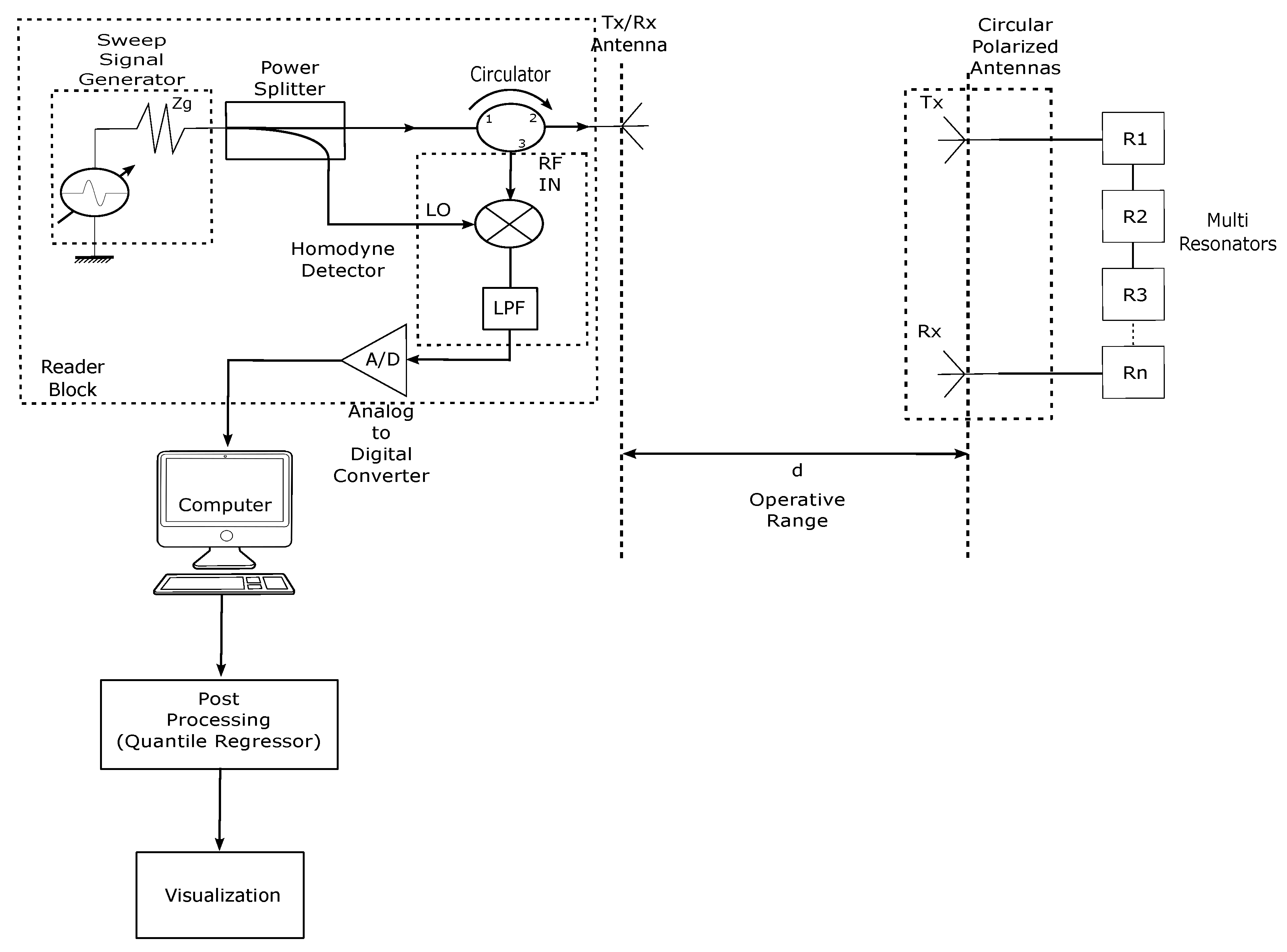
Figure 2.
Layout of the spiral resonator and the equivalent shunt resonator circuit.
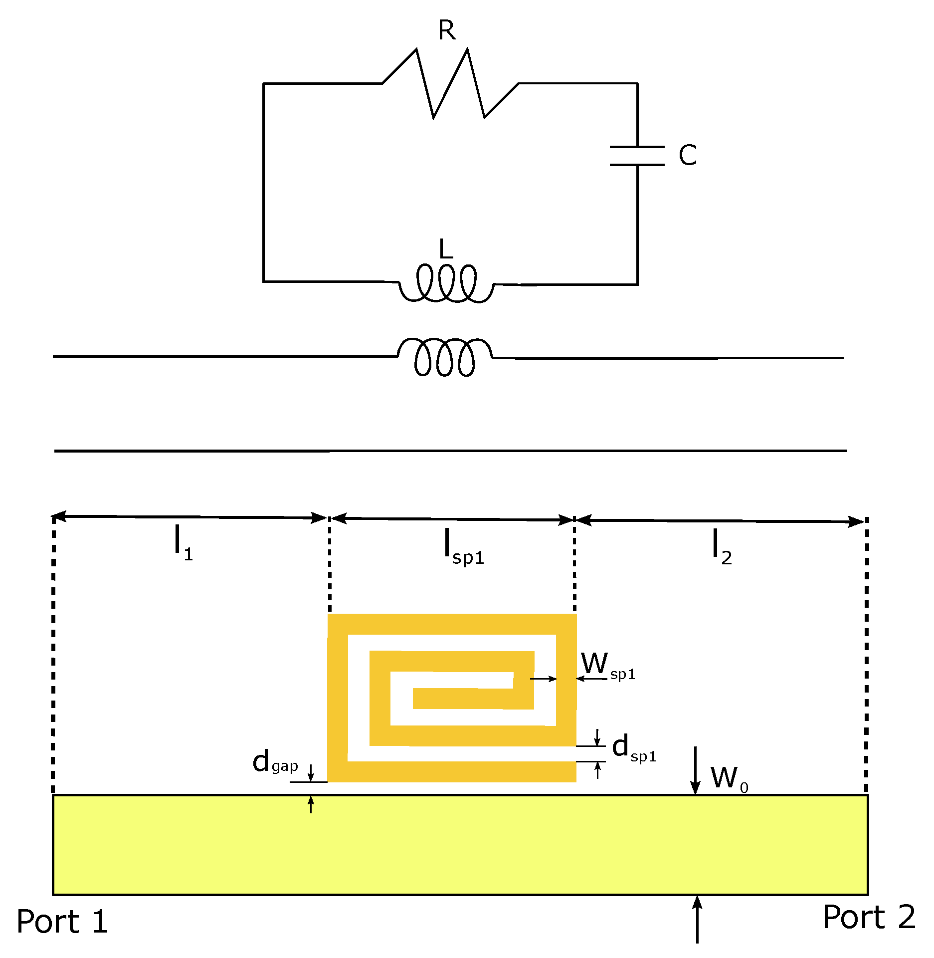
Figure 3.
Received 5-bit signal for the tag configuration of 11111.
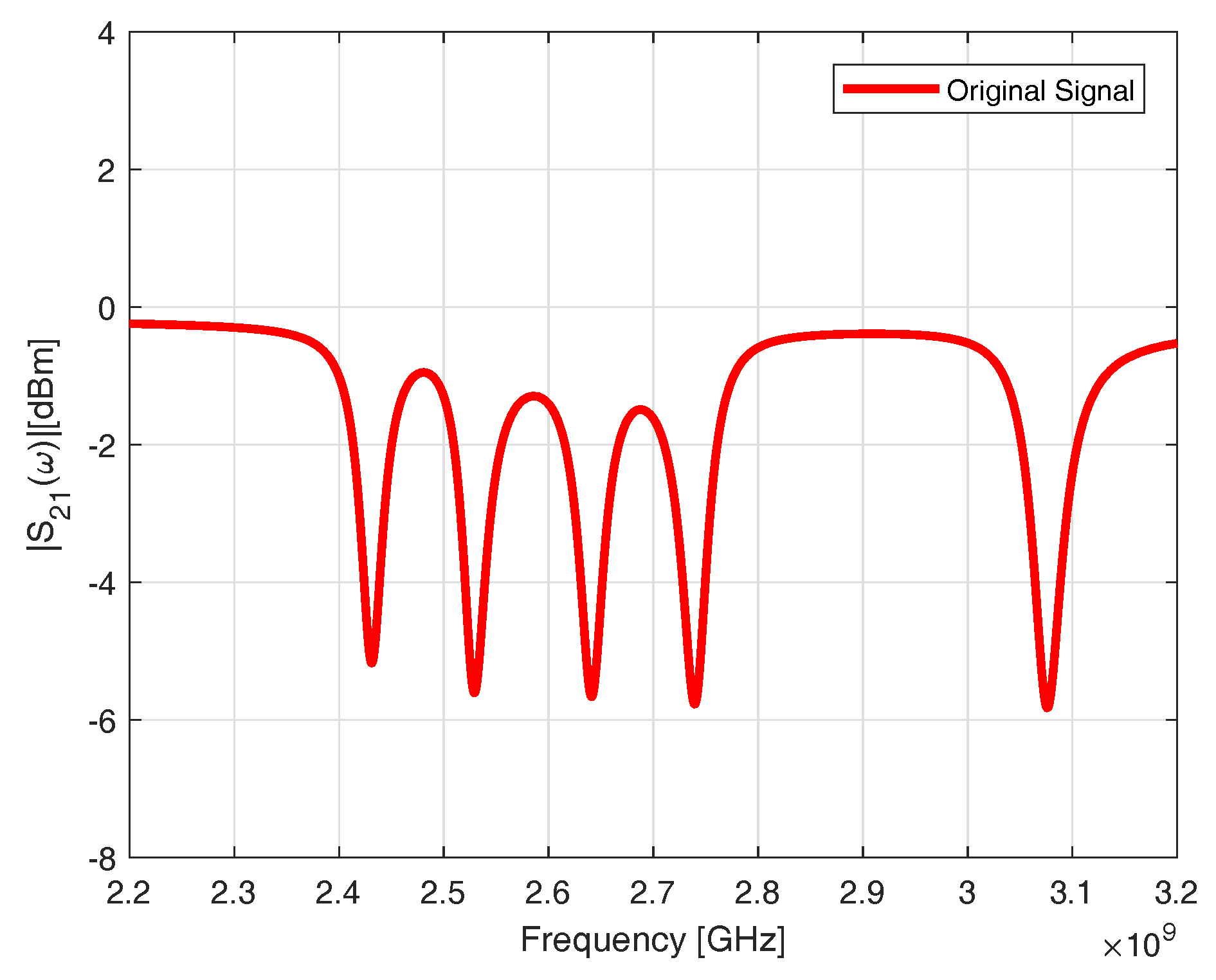
Figure 4.
Numerical assessment. Peak detected with the quantile regression, tag configuration 10110.
Figure 4.
Numerical assessment. Peak detected with the quantile regression, tag configuration 10110.

Figure 5.
Peak detected for the tag configuration of 10110, (a) original detected signal, peaks between the frequency range of (b) 2.4–2.5 GHz, (c) 2.6–2.7 GHz, (d) 3.1–3.2 GHz.
Figure 5.
Peak detected for the tag configuration of 10110, (a) original detected signal, peaks between the frequency range of (b) 2.4–2.5 GHz, (c) 2.6–2.7 GHz, (d) 3.1–3.2 GHz.
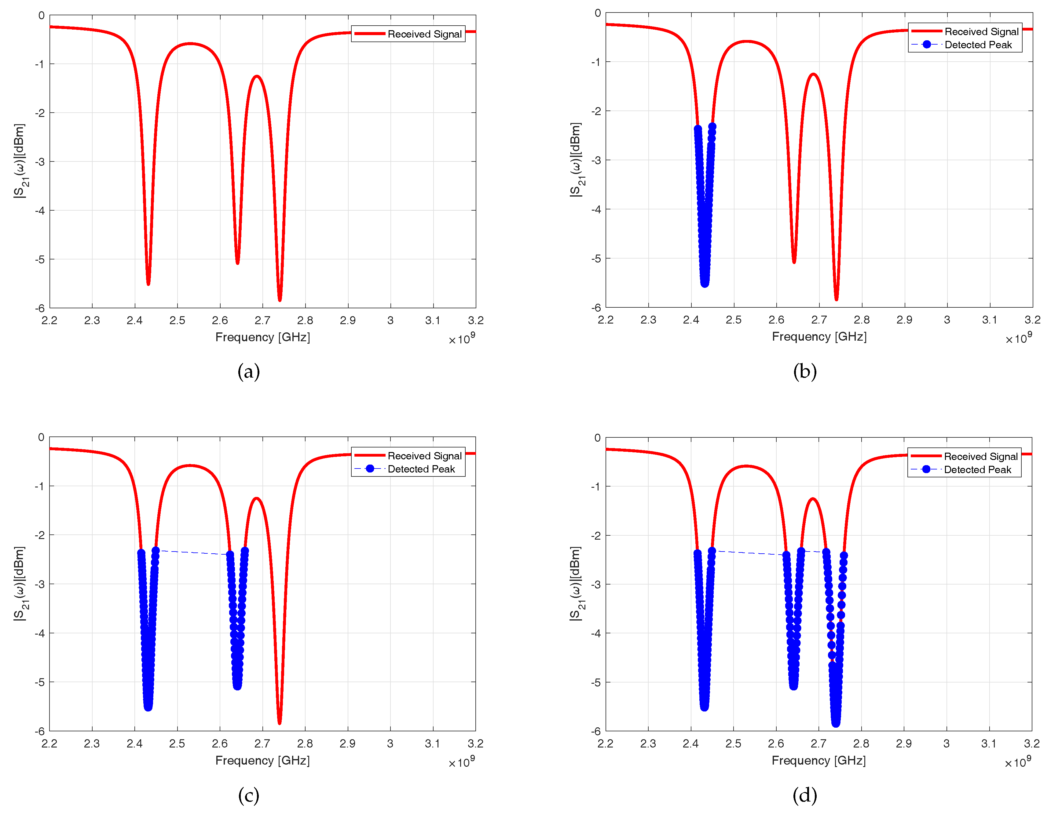
Figure 6.
Peak detected for the tag configuration of 00101, (a) original detected signal, between the frequency range of (b) 2.6–2.7 GHz, (c) 3.0–3.1 GHz, and (d) 2.2–3.2 GHz with a frequency shift at 3.1–3.2 GHz.
Figure 6.
Peak detected for the tag configuration of 00101, (a) original detected signal, between the frequency range of (b) 2.6–2.7 GHz, (c) 3.0–3.1 GHz, and (d) 2.2–3.2 GHz with a frequency shift at 3.1–3.2 GHz.

Figure 7.
Numerical assessment. Signal corrupted by additive white Gaussian noise (AWGN), frequency shift and peak amplitude random variations. Tag configuration 10110.
Figure 7.
Numerical assessment. Signal corrupted by additive white Gaussian noise (AWGN), frequency shift and peak amplitude random variations. Tag configuration 10110.
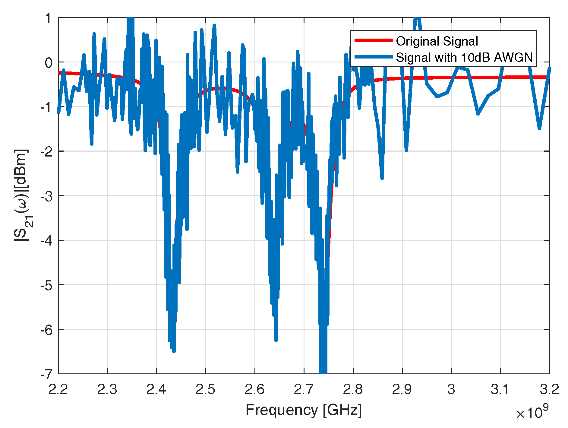
Figure 8.
Numerical assessment, noisy scenario. Peaks detected for the tag configuration of 10110, (a) original detected signal, peaks between the frequency range of (b) 2.6–2.7 GHz, (c) 3.0–3.1 GHz, (d) 3.1–3.2 GHz with frequency shift at 3.1–3.2 GHz, and (e) final step.
Figure 8.
Numerical assessment, noisy scenario. Peaks detected for the tag configuration of 10110, (a) original detected signal, peaks between the frequency range of (b) 2.6–2.7 GHz, (c) 3.0–3.1 GHz, (d) 3.1–3.2 GHz with frequency shift at 3.1–3.2 GHz, and (e) final step.

Figure 9.
A photo of the tag prototype demonstrator with five resonators and two broadband circularly polarized antennas.
Figure 9.
A photo of the tag prototype demonstrator with five resonators and two broadband circularly polarized antennas.
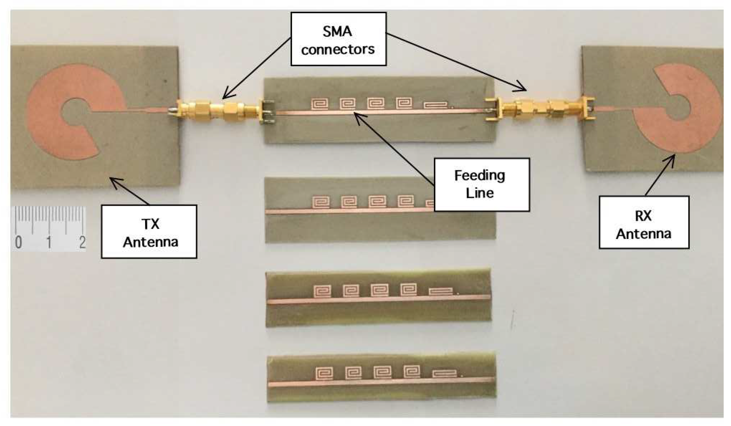
Figure 10.
The effects of resistive loads on the resonator response.
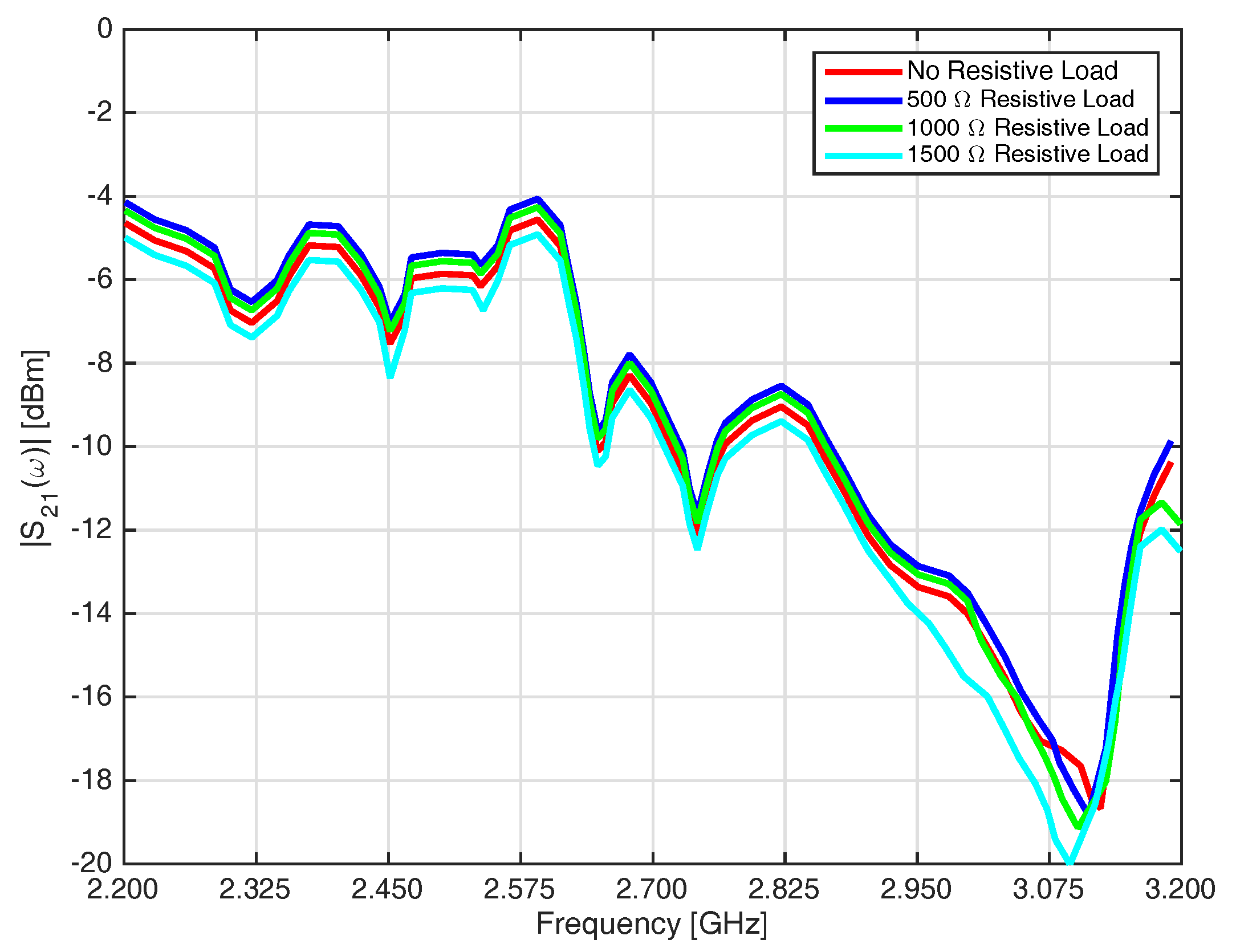
Figure 11.
Peak detection for the received real-time signal with the tag configuration of 11110 using the newly proposed method. (a) step 1, (b) step 2, (c) step 3,(d) step 4, and (e) final step.
Figure 11.
Peak detection for the received real-time signal with the tag configuration of 11110 using the newly proposed method. (a) step 1, (b) step 2, (c) step 3,(d) step 4, and (e) final step.
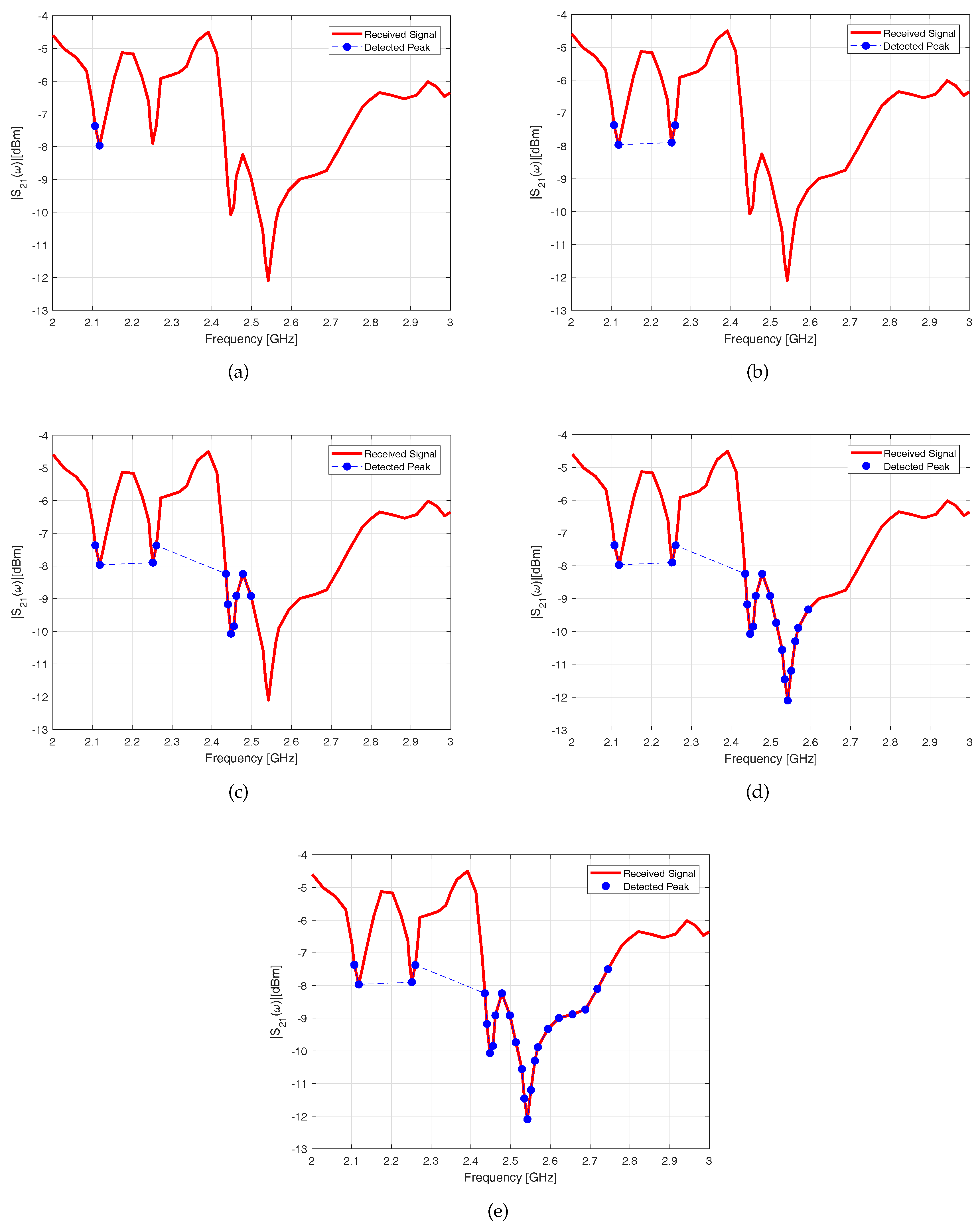
Figure 12.
Peak detection for the received real-time signal with the tag configuration of 11111 using the newly proposed method. (a) step 1, (b) step 2, (c) step 3,(d) step 4, and (e) final step.
Figure 12.
Peak detection for the received real-time signal with the tag configuration of 11111 using the newly proposed method. (a) step 1, (b) step 2, (c) step 3,(d) step 4, and (e) final step.


Table 1.
Design parameters of the five spiral resonators.
| Resonator | [GHz] | [mm] | [mm] | [mm] | [mm] | [mm] | |
|---|---|---|---|---|---|---|---|
| 1 | 2.4 | 80.1 | 9 | 7.48 | 0.7 | 0.3 | 0.1 |
| 2 | 2.5 | 76.5 | 9 | 7.18 | 0.7 | 0.3 | 0.1 |
| 3 | 2.6 | 73.5 | 9 | 6.9 | 0.7 | 0.3 | 0.1 |
| 4 | 2.7 | 71 | 9 | 6.65 | 0.7 | 0.3 | 0.1 |
| 5 | 3 | 66.3 | 9 | 5.95 | 0.7 | 0.3 | 0.1 |
© 2018 by the authors. Licensee MDPI, Basel, Switzerland. This article is an open access article distributed under the terms and conditions of the Creative Commons Attribution (CC BY) license (http://creativecommons.org/licenses/by/4.0/).
Share and Cite
MDPI and ACS Style
Manekiya, M.; Donelli, M.; Kumar, A.; Menon, S.K. A Novel Detection Technique for a Chipless RFID System Using Quantile Regression. Electronics 2018, 7, 409. https://doi.org/10.3390/electronics7120409
AMA Style
Manekiya M, Donelli M, Kumar A, Menon SK. A Novel Detection Technique for a Chipless RFID System Using Quantile Regression. Electronics. 2018; 7(12):409. https://doi.org/10.3390/electronics7120409
Chicago/Turabian StyleManekiya, Mohammedhusen, Massimo Donelli, Abhinav Kumar, and Sreedevi K. Menon. 2018. "A Novel Detection Technique for a Chipless RFID System Using Quantile Regression" Electronics 7, no. 12: 409. https://doi.org/10.3390/electronics7120409
Note that from the first issue of 2016, this journal uses article numbers instead of page numbers. See further details here.