Hyperspectral Image Classification Using Parallel Autoencoding Diabolo Networks on Multi-Core and Many-Core Architectures

Abstract

One of the most important tasks in hyperspectral imaging is the classification of the pixels in the scene in order to produce thematic maps. This problem can be typically solved through machine learning techniques. In particular, deep learning algorithms have emerged in recent years as a suitable methodology to classify hyperspectral data. Moreover, the high dimensionality of hyperspectral data, together with the increasing availability of unlabeled samples, makes deep learning an appealing approach to process and interpret those data. However, the limited number of labeled samples often complicates the exploitation of supervised techniques. Indeed, in order to guarantee a suitable precision, a large number of labeled samples is normally required. This hurdle can be overcome by resorting to unsupervised classification algorithms. In particular, autoencoders can be used to analyze a hyperspectral image using only unlabeled data. However, the high data dimensionality leads to prohibitive training times. In this regard, it is important to realize that the operations involved in autoencoders training are intrinsically parallel. Therefore, in this paper we present an approach that exploits multi-core and many-core devices in order to achieve efficient autoencoders training in hyperspectral imaging applications. Specifically, in this paper, we present new OpenMP and CUDA frameworks for autoencoder training. The obtained results show that the CUDA framework provides a speed-up of about two orders of magnitudes as compared to an optimized serial processing chain.

1. Introduction

Hyperspectral images are characterized by high spectral resolution, since they are acquired over hundreds of contiguous and narrow spectral bands [1]. Hyperspectral sensors produce as output a so-called hyperspectral data cube, where the x and y axes are the spatial dimensions and the z axis represents the spectral dimension. Therefore, hyperspectral sensors can acquire spatially and spectrally continuous data at the same time. A hyperpectral image acquired over L bands is made up of hyperspectral pixels. A hyperspectral pixel s, which has coordinates $(i,j)$, can be seen as an L-dimensional vector denoted as:

$$s_{i,j}=[s_{i,j}\left(1\right),s_{i,j}\left(2\right), \dots ,s_{i,j}\left(L\right)]\in {\mathbb{R}}^L$$

(1)

where $s_{i,j}\left(k\right)$ is the spectral response related to spectral channels $k=1, \dots ,L$. This issue paves the way to a wide range of applications in different fields such as agriculture [2], mineralogy [3], astronomy [4], chemistry [5], physics [6], surveillance [7], environmental monitoring [8] and medicine [9]. All those applications require to classify the hyperspectral pixels in a scene, to facilitate the decision process. It is important to note that hyperspectral data can provide higher classification accuracy than traditional imaging techniques [10]. However, there are critical issues related to hyperspectral imaging:

• the curse of dimensionality, which is due to the high spectral resolution;
• the large variability of the spectral signatures of the materials;
• the limited number of labeled training samples.

In the literature, the problem of hyperspectral data classification has been widely explored. There are works which exploit traditional classification algorithms such as minimum distance, maximum likelihood [11], logistic regression [12] and k-nearest-neighbors [13]. Other works exploit machine learning, such as traditional neural networks [14], SVM [15] and deep learning techniques [16]. Among these methods, unsupervised deep learning algorithms have emerged as a potential solution, since they do not need pre-labeled training samples. Autoencoders are gaining importance for this kind of classification tasks since their training is based on the reconstruction of a given image, without any labeled sample. Moreover, their capability to classify hyperspectral datasets has been widely demonstrated by different works [16,17]. The main issue in using autoencorders for hyperspectral image classification is that the training phase requires long periods in order to produce good results. This is due to the fact that the training is iterative (the mentioned operations are repeated several time until convergence) and, at each step, there is a back-propagation algorithm that updates the weights of the autoencoder. It is important to note that the involved operations are linear algebra routines. Therefore, parallel computing based on multi-core CPU and Graphical Processing Units (GPUs) can be exploited in order to reduce the training time of autoencoders [18]. Indeed, those parallel technologies have been already succesfully used for hyperspectral imaging and other scientific applications [19,20,21,22]. In particular, GPUs have been employed for images classification in [23,24,25].

In this paper, we present new parallel frameworks for autoencoder training in hyperspectral imaging applications by exploiting OpenMP and CUDA. Moreover, we compare the results obtained in terms of execution times of the proposed framework using different real hyperspectral images. Specifically, the main contribution of this paper is the development of two parallel frameworks for autoencoder training. In particular, we describe the design of autoencoders training through OpenMP and CUDA, exploiting in particular the cuBLAS library. The first one exploits multi-core architectures and is based on a set of compiler directives which point out the code parts to be automatically parallelized, while the latter requires a complete re-design of the application. The parallelization effort, of course, is completely different and more heavy for the CUDA framework. However, our experimental results show that the speed up obtained by CUDA is about two orders of magnitude larger than the one achieved by OpenMP. Moreover, we compare the performance of two different GPU architectures: the Kepler and the Volta, the last generation of NVIDIA arcitecture.

The remainder of the paper is organized as follows: Section 2 describes the autoencoders and the algorithm used for their training. It also depicts the proposed frameworks and Section 3 describes the obtained results and performs comparisons with related works. Finally, Section 4 concludes the paper and provides hints at plausible future research lines.

2. Materials and Methods

2.1. Supervised and Unsupervised Classification

In the literature, many works have focused on supervised classification, exploiting, among the other techniques, Support Vector Machines (SVM) [26,27], logistic regression [28] and Convolutional Neural Networks (CNN) [29]. Those techniques are quite different considering the operations needed to train the model and to classify a dataset. However, both rely on a group of pre-labelled samples, called training-set. The number of pre-labelled samples and their quality highly influence the final classification accuracy. This is a crucial issue which should kept in mind when choosing between supervised and unsupervised learning. In fact, remote sensing is a field where the availability of pre-labelled samples is limited; therefore, it is better to exploit techniques where no training-set is needed (i.e., unsupervised learning).

From the point of view of coding, being supervised or unsupervised does not directly affect the parallelization. This is because there is a wide range of algorithms belonging to both the categories, with significantly different operations. In the specific, if a technique relies on linear algebra operations and the data dimensionality is high, parallel computing techniques can be adopted in order to reduce processing times.

2.2. Autoencoders for Hyperspectral Image Classification

Autoencoders or Diabolo networks [30] are machine learning techniques which aim at reconstructing their own inputs. Those networks are characterized by an input layer, one or more small-dimensional hidden layers, and a reconstruction layer of the same size as the input layer. Each layer is made up of perceptrons or neurons. The weights from the input to the inner layer are called encoding weights, while those from the inner to the reconstruction layer are called decoding weights. Therefore, the network can be divided into two parts: the first performs an encoding process, while the latter performs a decoding one. The structure of the adopted autoencoder is shown in Figure 1. In this network, after the training phase, the classification is produced by the layer indicated as code in Figure 1.

The encoder produces, as output, the code, which is related to the classification of the input. The code is a layer made up of a number of neurons equal to the number of class to produce as output. During the encoding, a probability value is associated to each code neuron. The neuron with the highest value determine the class that is associated to the considered input. Concerning hyperspectral imaging, a class is a label which is assigned to the hyperspectral pixel given as input to the encoding network. The output of the classification of a whole hyperspactral image is a map of labels, indicating which pixels belong to the same class.

The training is performed by the back-propagation technique using as target the input data. Thus, there is no need of any pre-labeled data corresponding directly to the classes. In our case, the training is performed on a portion of the hyperspectral image to be classified.

The autoencoder receives as input an hyperspectral pixel, which is an L-dimensional vector and will be denoted with x hereinafter. The first part of the network performs the encoding. In this case, this portion of the network has a single hidden layer. Let $W_{ih}$ and $W_{hc}$ denote the matrix of the weights between the input and the hidden layers and the hidden and the code layers, respectively. If we denote with $h_1$ and with c the arrays of values assumed by the hidden and the code layers, respectively, the processing performed by the encoding network is given by:

$$\begin{array}{c}{h}_1=f(W_{ih}x+b_{ih})\end{array}$$

(2)

$$\begin{array}{c}c=f(W_{hc}{h}_1+b_{hc})\end{array}$$

(3)

where $b_{ih}$ and $b_{hc}$ are the biases and $f(·)$ is a non-linear activation function (in our case a sigmoid).

The decoding network performs similar operations. Let $W_{ch}$ and $W_{hr}$ be the weights matrix between the code and the second hidden layer and the weights matrix between the hidden and the reconstruction layers. If $h_2$ and r denote the arrays of values of the hidden and reconstruction layers, respectively, then the task performed by the decoding network is given by:

$$\begin{array}{c}{h}_2=f(W_{ch}c+b_{ch})\end{array}$$

(4)

$$\begin{array}{c}r=f(W_{hr}{h}_2+b_{hr})\end{array}$$

(5)

where $b_{ch}$ and $b_{hr}$ are the biases.

In order to train the network, a Cost Function (CF), similar to the Mean Squared Error (MSE) between a given input set and its reconstruction is calculated as:

$$CF=\frac{{\sum }_{i=1}^N{(x_i-r_i)}^2}{2N}$$

(6)

where N is the total number of training samples.

If the CF is above a suitable threshold, the weights should be adjusted, in order to provide a better classification accuracy. In this case, all the weights are updated by a classic delta rule, which is given by:

$$\Delta w_{ij}\left(n\right)=\eta {\delta }_j\left(n\right)y_j\left(n\right)+\mu \Delta w_{ij}(n-1)$$

(7)

where $\Delta w_{ij}\left(n\right)$ is the update of the weight in position $(i,j)$ at the iteration n, $\eta$ is the learning rate, ${\delta }_j\left(n\right)$ is the local gradient of the j-th neuron, $y_j\left(n\right)$ is the output of the j-th neuron, $\mu$ is the momentum and $\Delta w_{ij}(n-1)$ is the update performed at the previous iteration.

The CF does not always decrease in successive iterations, therefore, we adopted a suitable strategy in order to avoid CF oscillations. We evaluate CF after and before the weights update and compute the ratio between those two values. If this ratio is less than 1, the learning rate is increased and all the updated weights are stored. Otherwise, if the ratio is between 1 and 1.04, the new weights are stored but the learning rate does not change. Finally, if the ratio is greater than 1.04, the learning rate is decreased and the weights are discarded. The values 1 and 1.04 have been estimated empirically.

The training phase ends if the CF is below a fixed threshold or if the number of training iterations exceeds a maximum value. In summary, the steps of the adopted training algorithm are:

• Feed-forward phase for computing the reconstruction of a given input with the actual weights;
• Back-propagation phase for computing the updated weights;
• Feed-forward phase with the updated weights;
• CF computation of the first feed-forward step;
• CF computation of the second feed-forward step;
• Computation of the ratio between the two CFs and adjusting the learning rate;
• If the CF decreases, store the updated weights, otherwise discard the update.

At this point, the encoding network is able to classify the whole hyperspectral image.

An important issue of autoencoders is that they also provide data compression, since they are able to reconstruct the input using only the decoding network. Thus, the classification of a hyperspectral image through an autoencoder also allows image compression.

2.3. Parallel Frameworks for Efficient Autoencoder Training

In this work, we focus on parallelization of the training phase of autoencoders, since it is the heaviest part from the computational point of view. Concerning data classification (inference) it is performed by the coding network and it is not iterative. Therefore, as we will discuss later, its processing time is negligible with respect to training time.

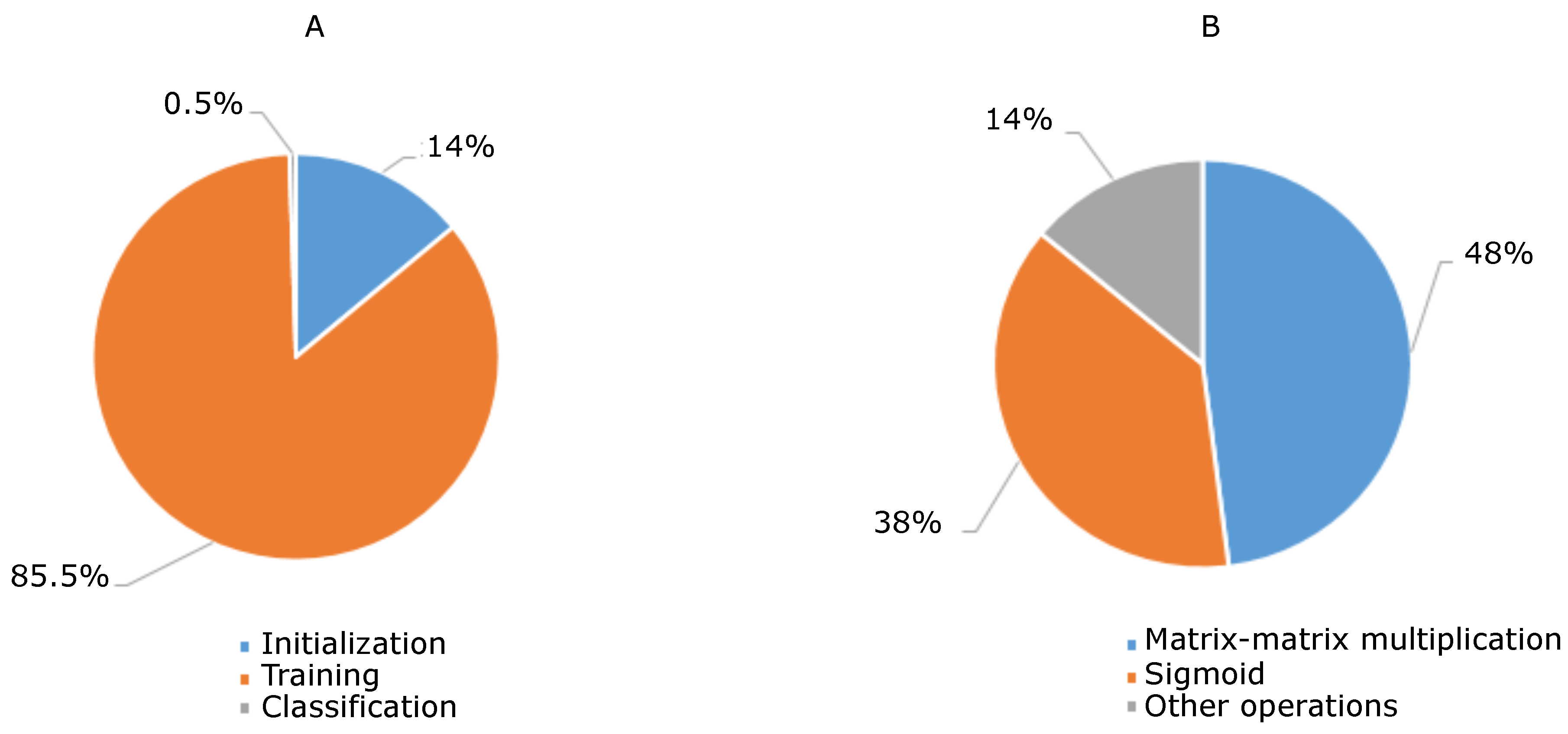
First, we developed a serial C implementation of the autoencoder described in the previous Section. This implementation serves as a baseline for the two newly developed parallel implementations. Moreover, it exploits the Advanced Vector Extensions 2 (AVX) instructions, in order to provide an optimized serial version. We choose to exploit multi-core and many-core architectures; in particular, for the first technology we adopted the OpenMP API, while for the latter we used the CUDA paradigm. The first solution has a lower parallelization effort when compared to the latter, but is not capable of achieving the same level of performance. Moreover, the serial implementation also allows us to perform a code profiling in order to identify the most time consuming operations. Profiling has been carried out using a real image with 300 × 300 pixels acquired over 33 bands. This image is smaller than the images that we used for testing our frameworks. However, even with an hyperspectral image of reduced sizes it is possible to notice how the computational weight is distributed among the different tasks. Those proportions are similar on bigger images. The training has been performed on a sub-image of suitable size. Therefore, the reconstruction needed for the training considers, as input, a sub-image stored as a matrix. This profiling highlights that the initialization and the selection of the training set took about 14% of the total processing time, while the training phase accounts for the 85.5%, and the rest is related to classification. Moreover, if we analyze only the training phase, 48% of the time is needed for matrix multiplication, while 38% is needed for the sigmoid function and the remaining 14% is needed for the other operations, such as memory allocations, random numbers generation and data normalization. This is shown in Figure 2.

It is important to note that the operations involved in the training phase are intrinsically parallel. The next two subsections describe the OpenMP API and CUDA frameworks for efficient autoencoders training.

2.3.1. OpenMP Framework

OpenMP is an API for shared memory system parallel programming. It is widely used for programming multi-core CPUs and its popularity is mainly due to the low parallelization effort that it requires when compared to other techniques. In particular, OpenMP is based on a series of pragma directives, used for serial code annotation. These annotations point out to the compiler which code portions should be automatically parallelized. An OpenMP application execution always starts from the master thread; when a parallel region is reached, a group of cooperating threads is defined in order to perform the desired task through a fork. When all the slave threads finish their task, they are joined and the execution continues in a serial way. These concepts are shown in Figure 3.

As already introduced, the adopted autoencoder is made up of five layers: one input layer, two hidden layers, a code layer and a reconstruction layer. The input layer simply stores the input values of each hyperspectral pixel. The other layers perform operations similar to Equation (2). Thus, each layer performs:

• a matrix–matrix multiplication;
• a matrix sum, in order to consider the bias;
• the evaluation of a sigmoid function for each element and the evaluation of the matrix resulting from the previous operations.

In order to optimize the number of performed operations, together with the memory accesses, we adopted a suitable data packing, which allows to compute the product between the inputs and the weights and the bias sum with a single matrix–matrix multiplication. In particular, we added a column to the weights matrix and a row of 1 s to the sub-image used for the training. In this way, performing the matrix–matrix multiplication is equivalent to compute the input to the sigmoid. Therefore, a generic weights matrix W and a generic input x can be written as:

$$W=\left[\begin{array}{cccc}{w}_{11}& \cdots & w_{1n}& b_1\\ w_{21}& \cdots & w_{2n}& b_2\\ \cdots & \cdots & \cdots & \cdots \\ w_{m1}& \cdots & w_{mn}& b_m\end{array}\right]X=\left[\begin{array}{ccc}{x}_{11}& \cdots & x_{1k}\\ x_{21}& \cdots & x_{2k}\\ \cdots & \cdots & \cdots \\ x_{l1}& \cdots & x_{lk}\\ 1& \cdots & 1\end{array}\right]$$

(8)

At this point, each layer is made up of a main for cycle which performs a matrix–matrix multiplication and an element-wise sigmoid of the resulting matrix for every feed-forward computation. The cycles have been parallelized by means of the #pragma omp parallel for OpenMP directive. The inner variables of each loop are declared private whilst the network structure is declared shared for the group of threads. The directive allows the programmer to set the scheduling of the threads. In this case, a static scheduling that divides the iterations into pieces of chunk size and then statically assigns the pieces to the threads was used. The chunk can be specified as a parameter of the directive; if it is omitted, the iterations are equally divided among all threads.

On the other hand, the back-propagation function is divided into two main parts: the first one calculates the error for each layer, while the second one updates the network weights. Error computation is performed through a single loop, which can be parallelized using the aforementioned directive. The weights update is performed through the Equation (7) and it can also be parallelized through the same directive. The learning rate update and the errors ratio computation are performed in a serial way, together with the stopping criteria test, since they are not heavy from a computational viewpoint.

The threads execute the same operations flow; therefore, in order to guarantee load balancing, each thread should work on the same data chunk. This is auto-tuneable by knowing the ratio between the data to be processed and the number of threads.

2.3.2. CUDA Framework

The GPUs manufactured by NVIDIA can be programmed to process general tasks (i.e., not necessarily related to graphics) through the CUDA API. The general philosophy of the different generations of GPUs developed by NVIDIA is to equip the devices with hundreds of cores grouped into so-called streaming multiprocessors. All the cores of a streaming multiprocessor share the on-chip memory, called shared memory, the registers and special purposes resources such as the Special Function Units (SFUs) which perform transcendental instructions. The last generation of NVIDIA architectures, codenamed Volta, also features tensor cores, optimized for deep learning operations, such as the ones involved in autoencoders training and classification phases.

In CUDA, the execution of the serial code parts are assigned to a traditional CPU, called host, while the parallel code parts are processed by the GPU, called device. The routines executed by the device are called kernels. A typical CUDA application is made up of five fundamental steps:

• Memory allocation on the device;
• Data transfers from the host memory to the device memory in order to give input data to the GPU;
• Kernel launch;
• Data transfers from the device memory to the host memory in order to retrieve the results from the GPU;
• Memory deallocation on the device.

The data transfers between host and device are carried out by the PCI-express bus. Thus, the minimization of data transfers is a critical issue in CUDA applications, since the PCI-express bus is typically a bottleneck. Thus, in our framework for autoencoder training, we properly managed memory transfers in order to minimize communications between the host and the device. The first step concerns the memory allocation and the data transfers. It is important to highlight that the data transfer from host to device is performed only once, before the beginning of the training. In particular, only the hyperspectral image is transferred. The weight matrices are only allocated, since their initialization is performed directly by the device. Typically, the weights are randomly initialized. Our proposal exploits the cuRAND library, which allows us to generate random uniform numbers directly on the device [31] through the curand_uniform routine.

The matrix–matrix multiplication has been implemented through the cuBLAS library [32]. Among the various routines of this library, there is the cublasDgemm routine, which computes the formula:

$$C=\alpha op\left(A\right)op\left(B\right)+\beta C$$

(9)

where A, B and C are matrices, $\alpha$ and $\beta$ are scalar values and $op(·)$ indicates the possibility of transposing the matrix. An important issue about cuBLAS library is that it works with matrices stored in column-major format, while in standard C matrices are usually stored in row-major format. It is easy to verify that the conversion from the first format to the latter one consists of a matrix transposition, thus a correct use of the $op(·)$ option allows to avoid the adoption of column-major format in the C code.

The feed-forward routine has been implemented by calling the cublasDgemm function for each layer. The weights matrix W and the input data X of the considered layer are passed to this routine, while $\alpha$ and $\beta$ are set to 1 and 0, respectively. In order to complete the task, it is necessary to evaluate the element-wise sigmoid of the matrix. Since there is no pre-built sigmoid routine, an “ad hoc” kernel has been developed which simply reads the data from the GPU memory, performs the computation and, finally, stores the result. In particular, each thread performs the sigmoid function through the formula:

$$f\left(x\right)=\frac{1}{1+e^{-x}}$$

(10)

where x is an element of the input matrix.

As already explained, the back-propagation algorithm requires the errors computation and the weights update. The first task is performed by the cublasDgeam function, which computes:

$$C=\alpha op\left(A\right)+\beta op\left(B\right)$$

(11)

where A, B and C are matrices, $\alpha$ and $\beta$ are scalar and $op(·)$ indicates the possibility of transposing the matrix. The error computation requires the difference between the elements of two matrices, therefore, $\alpha$ and $\beta$ are set to 1 and −1, respectively. The second phase, which implements Equation (7) consists of the following steps:

• Matrix–matrix multiplication between the weight matrix of the actual layer and the output of the previous layer performed by the cublasDgemm routine setting $\alpha =\eta$ and $\beta =0$;
• Sum between the matrix calculated at point 1 and the weight correction of the previous iteration. The sum is computed by the cublasDgeam routine setting $\alpha =1$ and $\beta =0$;
• the updated weight matrix is computed through the cublasDgeam routine setting $\alpha =1$ and $\beta =0$.

All the kernels are launched in batch for each image.

Finally, the convergence control is performed in the same way as in the OpenMP and serial versions.

3. Results and Discussion

The proposed frameworks have been tested with two real images. The first, which will be referred to hereinafter as PaviaU, is an image acquired over the University Campus of Pavia. The image is made up of 610 × 340 pixels acquired over 103 bands. The second one, that will be referred to hereinafter as PaviaC, is acquired over the city center of Pavia. It is made up of 1096 × 715 pixels acquired over 102 bands. A significative band among those present in the two images is shown, in black and white, in Figure 4. In the cases, we performed four different tests, with training sets corresponding to 1%, 10%, 30% and 50% of the pixels in the image.

Tests have been conducted on a PC equipped with an Intel${}^{\circledR }$ Core™i7 quad core processor working at 2.93 GHz and 8 GB of DDR3 RAM. The GPU is an NVIDIA Tesla K40, based on the Kepler architecture. it is equipped with 15 streaming multiprocessors, each one featuring 192 CUDA cores (for a total of 2880 cores) working at 750 MHz. A CUDA core is made up of an integer arithmetic logic unit and a floating point unit, both pipelined. The floating point unit fully supports IEEE 754-2008 single and double precision standards. The amount of available memory is 12 GB of DDR5 RAM. We also evaluate the most recent architecture by exploiting an NVIDIA Tesla V100 GPU. This board is connected to a node of the Galileo supercomputer hosted at the Cineca. It is equipped with 5376 cores organized into 84 streaming multiprocessors. It also features 672 tensor cores, 8 for each streaming multiprocessor. The working frequency is 1.45 GHz and the total amount of available memory is 16 GB.

Serial and OpenMP codes have been compiled on the PC using the Microsoft vc140 compiler, specifying compilation options to optimize the execution speed of the final application. The CUDA code has been compiled with the nvcc compiler, specifying the options in order to produce a code optimized for the considered GPU. Concerning the Tesla K40 board, we indicate to produce code optimized for the Kepler architecture using the flags -arch=compute_35 and -code=sm_35. On the other hand, for the Tesla V100 board, based on the Volta architecture, we used the flags -arch=compute_70 and -code=sm_70, which enables the use of the tensor cores for instructions such as cuBLAS routines. First, we checked that the outputs produced by the three versions are the same, considering equal initialization. The number of neurons in the hidden layers is set equal to $(2/3)L$, where L is the number of bands. The number of classes used is 10. The classification results obtained by the autoencoder, considering different percentages of the input for the training, for PaviaU and PaviaC are shown in Figure 5 and Figure 6, respectively.

The network is capable of recognizing the different details of an image only when it is trained with a suitable percentage of pixels in the image. As Figure 5 and Figure 6 show, a good classification is ensured only when the network is trained with a percentage ranging from 30% to 50%. Experiments with larger training sets have not been carried out, since there is a risk of over-training the network.

The performance evaluation of the three developed versions has been carried out by executing the training several times and calculating the mean of the processing times. Concerning the PaviaU image, the serial training took from about 1 h to about 3 days and 9 h when considering 1% of the image and 50% of the image for the training, respectively. Concerning the classification accuracy, it varies from 95% to 98%.

Table 1. Processing times for the PaviaU image. The speed-up is indicated with the abbreviation SU.

Training Set Size	Serial [s]	OpenMP	Tesla K40 [s]	Tesla V100 [s]	SU OpenMP	SU K40	SU V100
1% (1.63 MB)	4025.64	1690.31	159.22	107.85	2.38	25.28	37.33
	(1 h 7 m 6 s)	(28 m 10 s)	(2 m 39 s)	(1 m 47 s)
10% (16.30 MB)	42,558.15	15,967.14	373.69	164.83	2.66	113.88	258.19
	(11 h 49 m 18 s)	(4 h 26 m 7 s)	(6 m 14 s)	(2 m 45 s)
30% (48.90 MB)	207,547.13	62,284.18	991.15	423.69	3.33	209.94	486.41
	(2 d 9 h 39 m 7 s)	(17 h 18 m 4 s)	(16 m 31 s)	(7 m 4 s)
50% (81.50 MB)	288,028.63	78,254.06	1335.43	586.20	3.68	215.68	491.35
	(3 d 9 h 0 m 29 s)	(21 h 44 m 14 s)	(22 m 15 s)	(9 m 45 s)

and

Table 2. Processing times for the PaviaC image. The speed-up is indicated with the abbreviation SU.

Training Set Size	Serial [s]	OpenMP	Tesla K40 [s]	Tesla V100	SU OpenMP	SU K40	SU V100
1% (6.10 MB)	16,084.23	6740.80	630.22	309.71	2.39	25.52	51.93
	(4 h 28 m 4s)	(1 h 52 m 21 s)	(10 m 30 s)	(5 m 10 s)
10% (61.00 MB)	173,198.33	63,850.40	1465.83	665.51	2.71	118.16	260.25
	(2 d 0 h 6 m 38 s)	(17 h 44 m 10 s)	(24 m 26 s)	(11 m 05 s)
30% (183.00 MB)	830,170.31	248,137.14	3961.12	1690.26	3.34	209.58	491.15
	(9 d 9 h 39 m 7 s)	(2 d 20 h 55 m 37 s)	(1 h 6 m 1 s)	(28 m 10 s)
50% (305.00 MB)	1,150,012.14	313,014.57	5330.10	2336.66	3.67	215.76	492.16
	(13 d 7 h 26 m 52 s)	(3 d 14 h 56 m 54 s)	(1 h 28 m 50 s)	(38 m 57 s)

report the processing times measured after applying the three versions to the processing of PaviaU and PaviaC, respectively. Inference times are not reported since they are always less than 1 s; therefore, they are negligible with respect to training time.

The maximum available memory of the systems’ limits the size of the image to be classified. In particular, as said before, the OpenMP is tested on a PC equipped with 8 GB of RAM, while the CUDA version have been tested on an NVIDIA Tesla K40 equipped with 12 GB of RAM and on an NVIDIA Tesla V100 GPU with 16 GB of RAM. In all the cases, in the RAM memory, it is necessary to store the whole autoencoder layers weight, the training set and an auxiliary array for the back-propagation, whose dimensions are related to the training set and to the network dimensions. Moreover, during the classification, it is necessary to store the weight of the Encoder network, the whole hyperspectral image and the output classification map.

Concerning the OpenMP implementation, it is important to note that the speed-up increases and tends to the ideal value of 4 when considering a training set of about 50 MB. We also tried to increase to number of OpenMP threads but the processing times were longer if compared to the four threads version.

The CUDA application always performs better than the serial and the OpenMP applications, also when the training involves only 1% of the input data. This is because the error threshold that assures a good classification is very low (about ${10}^{-4}$); therefore, the number of training iterations is always high. The final reconstruction error is lower than the fixed threshold when considering a training percentage greater or equal than 10%. Also for the CUDA application, the speed-up increases with the dataset size. We performed a profiling of the CUDA application through the NVIDIA Visual Profiler.

These analyses highlight that the proposed framework minimizes the memory transfers, since they happen only at the beginning and at the end of the training, and they have a negligible weight with respect to the computation done on the device. Moreover, it shows that the GPU spends 77% of the time for the cublasDgemm routine, 8% for the cublasDgeam routine, 6% for the sigmoid and 9% for the other routines.

Concerning the parallelization effort, the CUDA framework development required longer time than the OpenMP one. Moreover, the programmer should be skilled with GPU computing, since different parallel libraries and custom code are mixed. In addition, the correct managing of data transfers is crucial for obtaining good results in these kinds of applications. In the considered project, a skilled programmer worked for about 2 months in order to develop the presented CUDA framework.

To the best of our knowledge, autoencoders have been already exploited in the context of hyperspectral imaging applications in [16,17,33]. The first work performs tests on an image similar to PaviaU and trains the autoencoder in less than 400 s, but it exploits a smaller network and the threshold used for the stopping criteria is not specified. However, we notice that only the 6% of the available training samples has been used for training. Moreover, the considered image is more regular and with less details with respect to PaviaU. The second work only analyses performance in terms of classification but does not report training times: therefore, it is not possible to perform a direct comparison between our implemenation and the proposal of [17]. Finally, ref. [33] proposed autoencoders for hyperspectral image classification showing how inference quality changes with respect to the training-set size, but training times are not reported.

In the literature, works about supervised learning [26,27,28,29] reported different values of speed-up, which are related to the specific board used and to the possibility of parallelizing the specific algorithm. Since the devices and the algorithms are different from the one considered in this paper, a direct comparison would be not fair. Moreover, it is important to consider that, as already said before, for supervised classification, pre-labelled training sets are necessary. This is a critical issue, because it is not always possible to have those labelled samples.

Finally, if we consider the features that affect code parallelization, our direct experience is that it depends on the characteristic of the specific algorithm under analysis. In our case, the training consists of linear algebra operations, which are intrinsically parallel and can be efficiently mapped on the GPU architecture. On the other hand, if we consider, as example, SVM training, there are some operations that required to evaluate conditions making the code diverge, which is not efficiently managed by the GPU architecture. Therefore, our results confirm that the characteristic of being supervised or unsupervised does not directly affect the exploitation of GPU technology, since there are very different techniques belonging to both the categories. In other words, the evaluation of parallel performance of an algorithm is related to the operations involved and to the data dimensionality.

4. Conclusions and Future Lines

In this paper, we presented two parallel frameworks for efficient autoencoder training in the context of hyperspectral imaging applications. In particular, we exploited OpenMP and CUDA API. The two frameworks have been tested with real hyperspectral images. The results show that the CUDA implementation performs better than the OpenMP version. Moreover, for an increasing training size, the OpenMP speed-up tends to the ideal value of 4 (we tested the application with a quad-core processor).

The CUDA framework has been evaluated with two different GPU architectures: Kepler and Volta. The first one is among the most widely used for scientific computation, while the latter represents the last family of NVidia GPUs released and features hardware optimizations for deep learning computations. Both devices obtained better performance with respect to the serial and the OpenMP code. In particular, the Tesla K40 achieves a maximum speed-up of about 210, while the Tesla V100 achieves a maximum speed-up of about 490. For both devices, the speed-up increases with respect to the training-set size. Moreover, the proposed CUDA framework outperforms the OpenMP and the serial one. It is important to note that the CUDA framework is the same for the two GPUs, therefore, the better performance of the Tesla V100 board is only related to the fact that the hardware is optimized (i.e., the presence of the tensor cores). This means that future architectures, which will include new and more tensor cores, will guarantee even lower training times than the Volta.

Finally, concerning the serial and the OpenMP versions, a better CPU (e.g., with more cores) will further reduce processing times. However, considering the obtained results, a better CPU would not perform as good as the GPU here, because the involved operations are intrinsically parallel and suitable for GPU computing.

Future work will probably be focused on developing parallel frameworks for other machine learning techniques, in order to develop a suite of parallel algorithms for efficient hyperspectral image classification.