Stability Driven Optimal Controller Design for High Quality Images

Abstract

This note presents an optimal design method to enhance image quality in optical image stabilization (OIS) systems. First of all, performance limitations of conventional methods are shown and secondly, a new design framework based on convex optimization is proposed. The resulting controller essentially stabilizes the closed loop systems because the proposed method is derived from Lyapunov stability. From the test results, it is confirmed that this method reduces the effect of hand vibrations and makes images sharp. Additionally, it is shown that the proposed method is also effective in robot vision and recognition rate of deep neural network (DNN) based traffic signs and pedestrians detection in automotive applications. This note has three main contributions. First, performance limitations of the conventional method are shown. Second, from the relation between sensitivity and complementary sensitivity functions, an indirect design method for performance improvement is proposed, and finally, stability guaranteed optimal design is proposed. Unlike conventional methods, the proposed method does not require addition filters to suppress resonances of the plant and this note highlights phases of the closed loop systems on removing external vibrations.

1. Introduction

This note focuses on optimal control design to achieve a wide bandwidth for high quality images in OIS systems. Performance limitations of the conventional methods are presented, and a new design framework to overcome the limitations is presented. In this section, background of this note, formulation of the problem of this study, a brief literature survey, the contribution of this study, and the organization of the manuscript are provided.

1.1. Background

Image-stabilization systems have been used in many applications, ranging from astronomical imaging to optical communications systems [1]. Recently, the technologies are being applied to consumer electronics such as digital cameras, digital camcorders, mobile phones and tablets. In mobile applications, hands vibrations make unwanted camera movements and the unwanted movements distort the optical path. In the camera, the distorted optical path is the reason for image quality degradation.

According to the image compensation method, image stabilization technologies are categorized into digital image stabilization (DIS) and optical image stabilization (OIS). In DIS, feature points and motion vectors are calculated, and several frames are aligned by using the motion vectors. For examples, a metric for evaluating fidelity, displacement and performance has been proposed [2], and fast electronic digital image stabilization system based on a two-dimensional feature-based multi-resolution motion estimation algorithm was presented. Stabilization is achieved by combining all motions from a reference frame and subtracting this motion from the current frame [3]. However, during DIS processing, loss of edge is inevitable in the corrected image. DIS requires application specific integrated circuit (ASIC) supporting DIS function, electrical power, and calculation time. However, compared to OIS, DIS is cost effective because it does not necessitate additional electrical components.

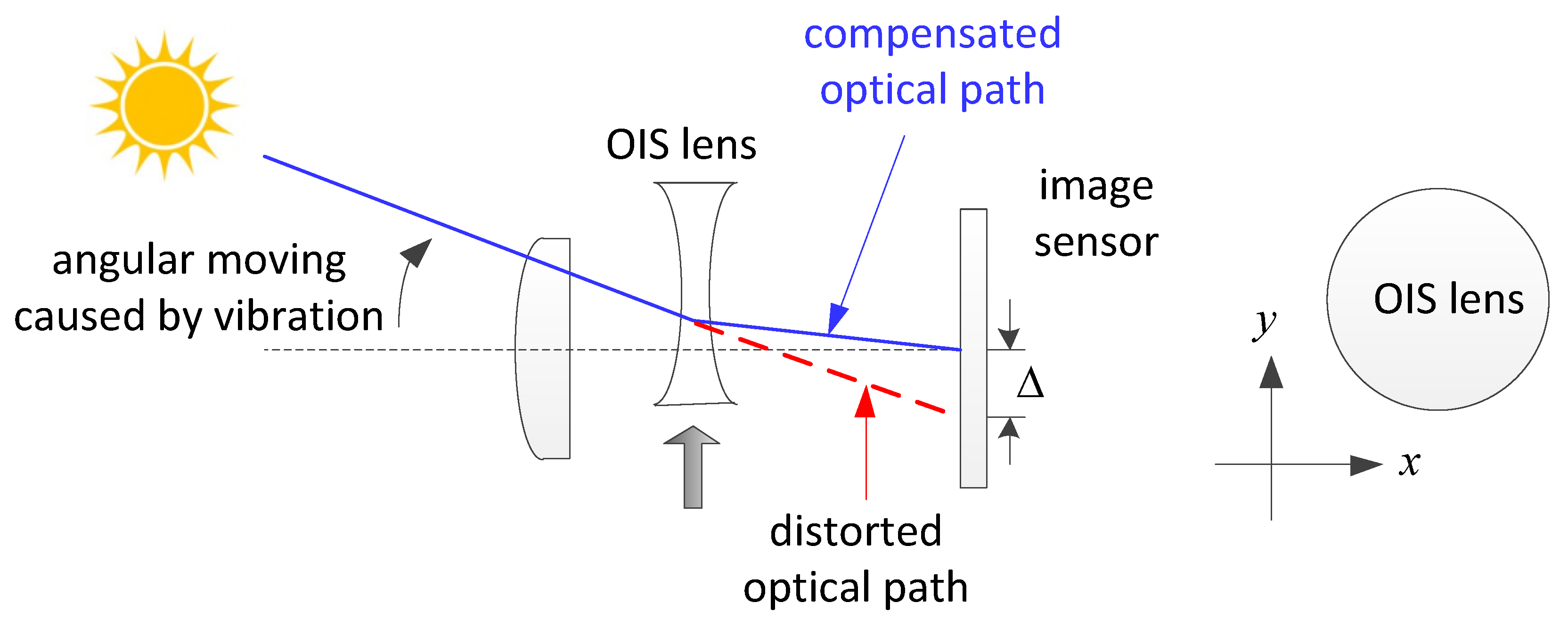
OIS systems directly correct the distorted optical path disturbed by hand vibrations. Sensors measure velocities and movements are calculated by using integral signal processing. In order to counteract the vibrations, the measured signal is utilized as a reference signal of the feedback control systems, and the control systems move the OIS compensation lens. The OIS lens should be able to move parallel to an image sensor because the vibrations are introduced in both directions. Figure 1 shows the mechanism. The introduced hand vibrations perturb the optical path, but the OIS lens compensates the distorted optical path and, finally, clear images are obtained. Compared to DIS, OIS requires additional sensors and actuators to control OIS systems, but in general, OIS is superior to DIS on the image quality.

In the latest cameras, image pixel size is decreasing for high image quality. However, the small pixel size makes the image quality more sensitive to the vibrations. Therefore, a more accurate and precise control algorithm is demanded.

1.2. Formulation of the Problem of Interest for this Investigation

In order to control XY two direction actuators, multi-input multi-out (MIMO) control methods and independent control along the single direction may be considered. MIMO control has been widely used for aircraft and process applications [4,5]. In this method, min/max singular values are utilized for design and analysis, but phase information cannot be used in general. In the independent control method, each controller is designed to meet design specification to the corresponding single axis actuator. In addition, the designed controller is augmented to build the two direction control systems. In this method, phase information can be used for design and analysis. In this note, the independent control method is used, and subscript x and y represent controller and plant for x and y directions.

In feedback control systems, a controller should be designed to meet design specifications and the specifications are determined by design objectives. However, even though the same design specifications are required, if the system types of plants to be controlled are different, the controller should be also differently designed to meet the same specifications. For example, suppose that with a given plant, command tracking is our design goal and a pole placement method is used as a controller. The designed controller is in the shape of a lead compensator and this means that the controller has a flat gain in the low frequency range. With such a controller, if the plant is type-0 (the plant has no pole at the origin), the open loop transfer function defined by multiplication of controller and plant has low gain in the low frequency range, resulting in poor command tracking performance. However, if the plant is type-1/2 (the plant has one or two poles at the origin), the open loop transfer function has high gain, resulting in good command tracking [6]. Therefore, before designing controllers, systems should be accurately identified and modeled. For those purposes, modal parameters were calculated, and it was confirmed that the computed parameters were good for plant modeling [7]. As a result, in order to meet design specifications, firstly the target plant should be analyzed, and secondly precise control should be designed.

1.3. Literature Survey

Since vibrations and oscillations are the source of the image quality degradation, the features of the vibrations should first be analyzed. As a study for oscillation, an analytical and computational framework based on the adjoint method for optimal open loop and closed loop control laws was proposed, and this method was applied to oscillating systems and successfully removed the oscillations [8]. OIS systems mainly consist of OIS actuators and their controllers. For the actuator affording better performances, the wide range of the linearity should be achieved, which was obtained by minimizing hysteresis [9]. Additionally, a sophisticated algorithm was also applied to design optimal actuators [10].

Along with developing the improved actuators, many controller design methods have been developed. Several decades ago, OIS control systems were already developed [11]. To remove global motions caused by hands or external disturbances, Kalman filtered smoothing of global camera motion has been employed and it was reported that process noise covariance has a direct effect on the operation of the stabilizer [12]. For cost effective CPU, instead of floating point CPU, 8bit fixed point controller was developed [13]. The lead-lag controller was also implemented on field programmable gate array (FPGA). In the designer friendly FPGA board, the poles and zeros were designed by design specifications, such as percentage overshoot, settling time, and damping ratio. PID control was used as well. In order to reduce the vibrations, multi-rate PID control was developed and the designed controller can reduce power consumption. Thus, it was said to be applicable to mobile applications [14]. In addition, drift compensation filter (DCF) to reduce the DC component of gyro sensor output was developed including PID controllers [15]. In [16], hand vibrations were measured and modeled by using Discrete Fourier Transform (DFT). In the paper, as plant modeling, second order systems were used. As a modern controller, current estimator based state feedback control was also developed [16]. However, these conventional methods have limitations on improving the performance of the closed loop systems because the designed controllers do not take flexible shapes to the given plant models, i.e., OIS actuators.

For the flexible control method, linear matrix inequality (LMI) based optimal controls have been developed [17,18,19] and the method has been widely used for mathematical estimation including optimal control design. It was reported that LMI can be used for identification and estimation. LMI can be also used for model identification [20]. To calculate the fault estimation algorithm, additional design constraints were faced, which could not be solved with typical methods. However, after the problem was modified into the LMI form, a solution could be found [21]. LMI based particle swarm optimization algorithm was also used to solve the distributional robust chance constrained model in wind power estimation [22]. For controller design, LMI is also used. In [23], LMI was used for control and stability analysis. Several sufficient conditions on stability and robust stability for sampled-data systems and the uncertain sampled-data systems, respectively, have been provided in terms of LMI. In an urban environment with heavy traffic, the transient current of battery of the small-sized electric car is controlled by multi-objective L2-gain, which is formulated by LMI [24]. In wind generation systems, the stability problems were reduced to a linear matrix inequality (LMI) problem and the current controller was also designed by the LMI method [25]. For model predictive control (MPC) of a quad-rotor platform, control took the form of linear matrix inequalities [26]. LMI control was used for trajectory tracking instead of iterative learning control (ILC) [27].

1.4. Scope and Contribution of this Study

This note proposes an optimal design method to enhance image quality in OIS systems. First, performance limitations of the conventional methods are proposed and secondly a new optimal method based on convex optimization is proposed. Since the proposed controller takes a flexible shape, it can easily shape the closed loop systems, resulting in wide closed loop systems. No other paper presents the performance limitations of the conventional methods and optimal solutions in OIS systems. Image quality tests verify that the proposed method is apparently effective to reduce the influences of the hand vibrations, resulting in clear and sharp images.

We summarize contributions of the note as follows.

• It is shown that the conventional methods have performance limitations on designing flexible frequency responses because the plant to be controlled is type-0 system.
• From the relationship between sensitivity and complementary sensitivity functions, an indirect design method for performance improvement is proposed and optimal design framework is suggested.
• In order to reduce the plant resonance, the proposed method does not require any additional filters.
• The proposed method always satisfies the closed loop systems stability because the method is based on Lyapunov stability.
• Unlike conventional methods, this note especially highlights phase responses of the closed loop systems.

The proposed method is especially effective at night because exposure time of the camera is longer, and more vibrations are introduced at night. Thus, this method is also applicable to automotive applications including consumer electronics.

1.5. Organization of the Manuscript

The rest of the note is organized as follows. Section 2 analyzes a plant model and evaluates the frequency response. In Section 3, convention design methods are presented. In the design of the conventional controllers, a notch filter is introduced to suppress a resonance peak and the limitation of the design flexibility is discussed. Section 4 contains a main idea, which is a flexible controller design method based on convex optimization. In Section 5, image quality tests are performed by using standard ISO resolution chart and in Section 6, the conclusions follow.

2. Plant Model

OIS requires two actuators because the lens for OIS should move in the XY-plane independently. Additionally, the model of OIS along the single axis in the continuous time domain is represented by second order systems

$$H(\mathrm{s})=\frac{{\omega }_n^2}{s^2+2\varsigma {\omega }_{n}s+{\omega }_n^2}\cdot G=\frac{2.527\times {10}^4}{s^2+75.4s+1.421\times {10}^5}$$

(1)

where $\varsigma =0.1,{\omega }_n=2\cdot \pi \cdot 60$ and $G=0.1778$ are damping ratio, natural frequency, and actuator driver gain, respectively [28,29]. Throughout the note, single axis systems are only considered, and the designed single axis controller is expanded to parallel systems.

3. Performance Analysis of Conventional Methods

The identified model is lightly damped systems. Therefore, in the conventional method, a notch filter is firstly designed to suppress oscillated responses of the plant as follows.

$$N(\mathrm{s})=\frac{s^2+2\varsigma {\omega }_{n}s+{\omega }_n^2}{s^2+2{\varsigma }_{\mathrm{mod}}{\omega }_{n}s+{\omega }_n^2}=\frac{s^2+75.4s+1.421\times {10}^5}{s^2+533.1s+1.421\times {10}^5}$$

(2)

Note that a numerator of $N(\mathrm{s})$ cancels out the denominator of $H(\mathrm{s})$ and applies a new denominator, $s^2+2{\varsigma }_{\mathrm{mod}}{\omega }_{n}s+{\omega }_n^2$. ${\varsigma }_{\mathrm{mod}}=0.707$ is selected as a new and modified damping ratio because with the damping ratio of 0.707, settling time and overshoot are absolute minimum in the second order systems as shown in Figure 2.

With $N(\mathrm{s})$, combined $H(\mathrm{s})\cdot N(\mathrm{s})$ becomes well damped systems, which is utilized for conventional controller design.

Figure 3 shows their frequency responses and it is shown that the notch filter suppresses a frequency peak of $H(\mathrm{s})$. Now, $H(\mathrm{s})\cdot N(\mathrm{s})$ is identified and modeled by new second order systems. Zero order hold discrete time equivalent models of the two actuators in the state space are given by

$$P_{x,y}=\{\begin{array}{c}{x}_{x,y}(k+1)=A_{x,y}{x}_{x,y}(k)+B_{x,y}{u}_{x,y}(k)\\ y_{x,y}(k)=C_{x,y}{x}_{x,y}(k)\end{array}$$

(3)

where $A_{x,y}\in {\Re }^{2\times 2},B_{x,y}\in {\Re }^{2\times 1},C_{x,y}\in {\Re }^{1\times 2}$ and both $\left(A_x,B_x,C_x\right)$ and $\left(A_y,B_y,C_y\right)$ are stabilizable and detectable and

$$A_{x,y}=\left[\begin{array}{cc}0.9315& 0.0009\\ -133.6772& 0.8606\end{array}\right],B_{x,y}=\left[\begin{array}{c}0.0122\\ 23.7715\end{array}\right],C_{x,y}=\left[\begin{array}{cc}1& 0\end{array}\right],D_{x,y}=0.$$

Since OIS systems are two-input and two-output systems, augmented systems P and corresponding controllers C could be described as follows.

$$P=\left[\begin{array}{cc}{P}_x& 0\\ 0& P_y\end{array}\right],C=\left[\begin{array}{cc}{C}_x& 0\\ 0& C_y\end{array}\right]$$

(4)

$C_x$ and $C_y$ are controllers for X/Y axes respectively.

As conventional controllers, lead-lag, PID, pole placement, and current estimator based pole placement were developed. However, these controllers take limited shapes to the given second order systems, $P_{x,y}$ as follows.

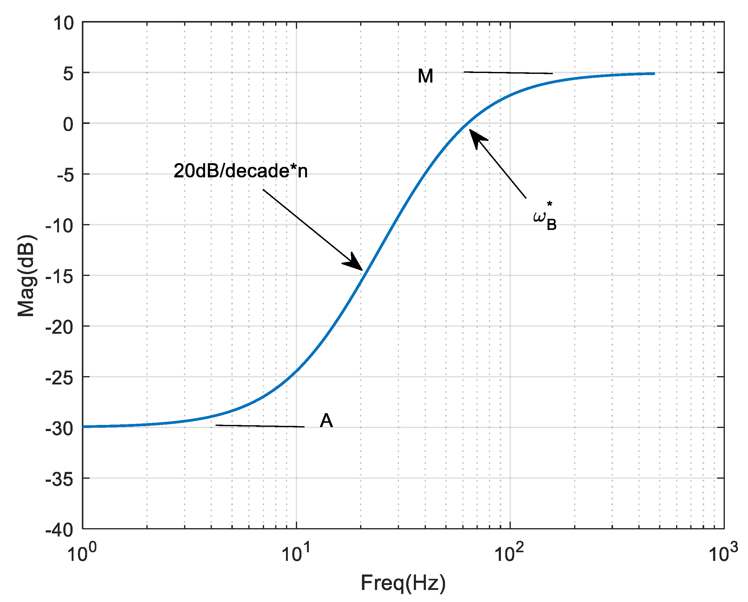
In the controllers, there may be one or two slopes in the frequency responses as shown in Figure 4. The slope in the high frequency affords stability margins whereas the slope in the low frequency plays a role in command tracking performances. Therefore, in order to obtain better performances in OIS systems, the slope in the low frequency should be steep or the command tracking area should move to the right-side more. However, in that case, stability might be easily broken because the moving slope encroaches on stability area. As an alternative, steeper slope in the low frequency, such as −40 dB/decade, might be considered, but in the conventional controller it is nearly impossible because the slopes should be a fixed value of ±20 dB/decade.

This limitation is caused by frequency responses of a plant and a controller. The plant (1) is a spring-mass-damper typed second order system, and this means slope of the low frequency gain is 0 dB/decade. With the given plant, conventional controller cannot make the open loop function with −40 dB/decade. Figure 5 explains the characteristics.

With lead or pole placement control, low frequency slopes of the open loop function is 0 dB/decade. If PID or lead-lag control is used, the low frequency slope would be −20 dB/decade. Thus, with the conventional controllers, the maximally achievable slope is −20 dB/decade. The gentle slope of the open loop transfer function limits the performance of command tracking. In this note, as a conventional controller $C_{conv}$, current estimator based pole placement control is used.

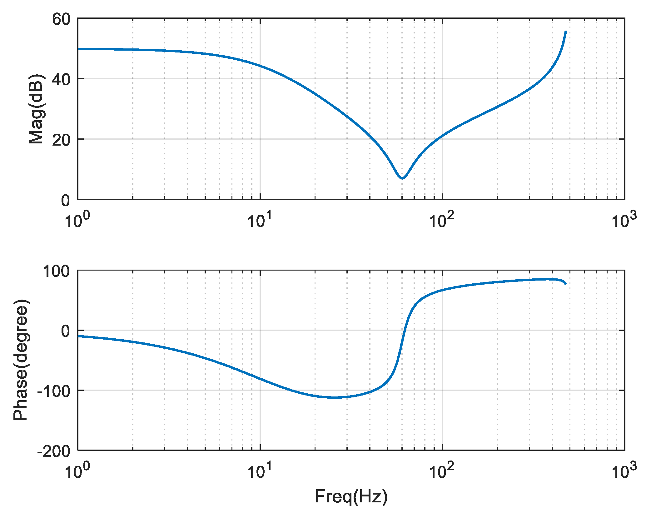
Note Figure 6. For good command tracking, sensitivity function should move to the right-side. However, if the slope of the open loop function is slow, sensitivity function cannot move to the right-side, and therefore, wide bandwidth closed loop function cannot be obtained. Therefore, since conventional controllers (PID or lead-lag case) have a maximum of −20 dB/decade in the low frequency range, such wide band closed loop systems cannot be designed.

4. Proposed Optimal Control

In order to obtain good image quality, command tracking performance is critical. For the good command tracking, a wide closed loop transfer function, i.e., scaled complementary sensitivity function T, should be designed and it can be obtained by a narrow sensitivity function S.

$$T+S=1$$

(5)

Equation (5) implies that T and S cannot be made small simultaneously. Therefore, if S could be smaller, then T could be larger [4]. Additionally, this means that influences induced from hand vibrations can be reduced and accordingly sharp images can be obtained.

To design wide bandwidth closed loop systems, S should be narrow without destroying stability and it is obtained by considering closed loop systems with fictitious output vibrations $d_x$ as shown in Figure 7. Note that $d_x$ is not a real hand vibration but a virtual vibration defined to enlarge a bandwidth of the closed loop systems.

In addition, transfer functions are represented as follows.

$$\begin{array}{l}T=\frac{y_x}{r_x}=\frac{P_x{C}_x}{1+P_x{C}_x}\\ S=\frac{y_x}{d_x}=\frac{1}{1+P_x{C}_x}\\ \frac{z_x}{d_x}=\frac{y_x}{d_x}\cdot \frac{z_x}{y_x}=\frac{y_x}{d_x}\cdot W_x^{-1}=S\cdot W_x^{-1}\end{array}$$

(6)

Equation (6) means that Equation (5) holds and S could take the form of $W_x^{-1}$ [17,18], and additional features, such as special band disturbance rejection and DC bias rejection, $W_{x,i}^{-1}$ could be added in $W_x^{-1}$ by simply multiplying corresponding functions [19], which affords flexible design. Composite $W_x^{-1}$ is designed as follows. First of all, desired frequency responses are collected independently, and the features are described by mathematical representations, $W_{x,i}^{-1}$. Accordingly, desired sensitivity function could be designed by

$$W_x^{-1}=W_{base}^{-1}\cdot {\displaystyle \prod _{i=1}^N{W}_{x,i}^{-1}}$$

(7)

where $W_{base}^{-1}$ is for base line design of sensitivity function. In this note, since only closed loop systems design with a wide bandwidth is addressed, the additional features are omitted.

To design such closed loop systems, $W_x^{-1}$ is written by

$$W_x^{-1}=D\left(\frac{{\left(s/M^{1/n}+{\omega }_B^{*}\right)}^n}{{\left(s+{\omega }_B^{*}\cdot A^{1/n}\right)}^2}\right)$$

(8)

where $D(\cdot )$ is a discretization operator with 1 kHz sample frequency. M and A are upper and lower bound of $W_x^{-1}$ and ${\omega }_B^{*}$ is a zero dB cross over frequency [4]. In addition, a detailed illustration is given in Figure 8.

With $u(\mathrm{k})=u_x(\mathrm{k})$, $y(\mathrm{k})=y_x(\mathrm{k})$ and $z(\mathrm{k})=z_x(\mathrm{k})$, state space representations of $P_x,W_x^{-1}$ are defined by

$$\begin{array}{l}{P}_x=\{\begin{array}{l}{x}_P(\mathrm{k}+1)=A_P{x}_P(\mathrm{k})+B_{P}u(\mathrm{k})\\ y_p(\mathrm{k})=C_p{x}_p(\mathrm{k})+D_{p}u(\mathrm{k})\end{array}\\ W_x^{-1}=\{\begin{array}{l}{x}_W(\mathrm{k}+1)=A_W{x}_W(\mathrm{k})+B_W{u}_W(\mathrm{k})\\ y_W(\mathrm{k})=C_W{x}_W(\mathrm{k})+D_W{u}_W(\mathrm{k})\end{array}\end{array}$$

(9)

where state space parameter of $W_x^{-1}$,$A_W,B_W,C_W,D_W$ is determined during design of $W_x^{-1}$, and plant parameter is given by

$$A_P=\left[\begin{array}{cc}0.9315& 0.0009\\ -133.6772& 0.8606\end{array}\right],B_P=\left[\begin{array}{c}0.0122\\ 23.7715\end{array}\right],C_p=\left[\begin{array}{cc}1& 0\end{array}\right],D_p=0.$$

Then, $z_x(\mathrm{k})$ depicted in Figure 7 is calculated by

$$\begin{array}{ll}{z}_x(\mathrm{k})& =C_W{x}_W(\mathrm{k})+D_W{u}_W(\mathrm{k})\\ & =C_W{x}_W(\mathrm{k})+D_W\left(y(\mathrm{k})+d_x(\mathrm{k})\right)\\ & =C_W{x}_W(\mathrm{k})+D_W\left(C_p{x}_p(\mathrm{k})+D_p{u}_x(\mathrm{k})+d_x(\mathrm{k})\right)\\ & =D_W{C}_p{x}_p(\mathrm{k})+C_W{x}_W(\mathrm{k})+C_W{x}_W(\mathrm{k})+d_x(\mathrm{k})+D_W{D}_p{u}_x(\mathrm{k})\end{array}$$

(10)

$y_x(\mathrm{k})$ and $x_P(\mathrm{k}+1)$ are also captured by

$$\begin{array}{l}{y}_x(\mathrm{k})=C_p{x}_p(\mathrm{k})+D_p{u}_x(\mathrm{k})+d_x(\mathrm{k})\\ x_P(\mathrm{k}+1)=A_P{x}_P(\mathrm{k})+B_P{u}_x(\mathrm{k})\end{array}$$

(11)

Finally, $x_W(\mathrm{k}+1)$ is calculated as follows.

$$\begin{array}{ll}{x}_W(\mathrm{k}+1)& =A_W{x}_W(\mathrm{k})+B_W{u}_W(\mathrm{k})\\ & =A_W{x}_W(\mathrm{k})+B_W\left(y_x(\mathrm{k})+d_x(\mathrm{k})\right)\\ & =A_W{x}_W(\mathrm{k})+B_W\left(C_p{x}_p(\mathrm{k})+D_p{u}_x(\mathrm{k})+d_x(\mathrm{k})\right)\\ & =B_W{C}_p{x}_p(\mathrm{k})+A_W{x}_W(\mathrm{k})+B_W{d}_x(\mathrm{k})+B_W{D}_p{u}_x(\mathrm{k})\end{array}$$

(12)

Using Equations (10), (11), and (12), augmented systems are represented by

$$\begin{array}{l}x(\mathrm{k}+1)=Ax(\mathrm{k})+B_1{d}_x(\mathrm{k})+B_2{u}_x(\mathrm{k})\\ z_x(\mathrm{k})=C_{1}x(\mathrm{k})+D_{11}{d}_x(\mathrm{k})+D_{12}{u}_x(\mathrm{k})\\ y_x(\mathrm{k})=C_{2}x(\mathrm{k})+D_{21}{d}_x(\mathrm{k})+D_{22}{u}_x(\mathrm{k})\\ \mathrm{where}x(\mathrm{k})={\left[\begin{array}{cc}{x}_P^T(\mathrm{k})& x_W^T\end{array}(\mathrm{k})\right]}^T\mathrm{and}\\ A=\left[\begin{array}{cc}{A}_p& 0\\ B_W{C}_P& A_W\end{array}\right],B_1=\left[\begin{array}{c}0\\ B_W\end{array}\right],B_2=\left[\begin{array}{c}{B}_P\\ B_W{D}_P\end{array}\right],\\ C_1=\left[\begin{array}{cc}{D}_W{C}_P& C_W\end{array}\right],D_{11}=D_W,D_{12}=D_W{D}_P,\\ C_2=-\left[\begin{array}{cc}{C}_P& 0\end{array}\right],D_{21}=-1,D_{22}=-D_P.\end{array}$$

(13)

For designing $C_x$, Lyapunov stability based convex optimization is used. Thus, $C_x$ always stabilizes the closed loop systems.

Using Equation (13) and a linear program, an optimal controller is calculated as shown in Figure 9. In the low frequency range, a gain is sufficiently high, which means designed controller yields good command tracking performances. In the high frequency range, features of the phase-lead control are observed, which affords stability margins, resulting in stable closed loop systems. The other feature is also observed at 60 Hz. That is a typical form of the notch filter. However, throughout the note, no notch filer has been designed in the proposed method. These positive features have been simultaneously obtained in the proposed framework as shown in Equation (13).

Compared conventional design methods, these characteristics are more obvious.

In the conventional controller design, a notch filter is firstly applied to the plant to suppress a frequency peak and then feedback control is secondly designed. Therefore, the finally designed controller is composed of the notch filter and the feedback controller. Figure 10 displays the composite frequency responses. The composite controller $Notch\cdot C_{conv}$ yields stability margins in the high frequency range, and it takes the form of a notch filter at the resonance frequency of the plant. However, the gain in the low frequency is still low and this incurs performance degradation on the command tracking, but the proposed method affords all these features at once.

5. Numerical Example and Discussions

In this simulation, an ideal pinhole camera model was used. As simulation parameters, object distance defined by a distance between an object and a pinhole was 1 m and focal length defined by a distance between the pinhole and an image sensor was 1.9 mm because a mobile phone was considered. In addition, rotational vibration of hands is defined by 1 degree, which was measured from lab tests. Then, the deviation from the optimal optical path Δ was calculated by 1.9 mm/180 = 10.6 μm. For numerical example, Equation (3) is used for plants for both x- and y-direction control, i.e., $P_x=P_y$. Additionally, for two-dimensional movements, the plants were augmented as shown in Equation (4). Similarly, the corresponding controller was independently designed and augmented as shown in Equation (4). In this example, two controllers have same frequency responses, i.e., $C_x=C_y$.

To design wide bandwidth closed loop systems, equivalently, narrow bandwidth sensitivity function, desired sensitivity function was designed by using Equation (8). In this application, $n=4$, $M={10}^{\left(-5/20\right)},A={10}^{\left(30/20\right)},{\omega }_B^{*}=2\pi \cdot 17$ were selected to obtain high gain open loop function and a narrow band sensitivity function and designed parameters are shown in Equation (14). The designed weighting function and its state space representation of Equation (9) are as follows. For discretization operator, matlab command ‘c2d’ was used.

$$\begin{array}{l}{W}_x^{-1}=D\left(\frac{{\left(s/M^{1/n}+{\omega }_B^{*}\right)}^n}{{\left(s+{\omega }_B^{*}\cdot A^{1/n}\right)}^n}\right)=D\left(\frac{s^4+370s^3+5.133\times {10}^4{s}^2+3.166\times {10}^{6}s+7.32\times {10}^7}{0.5623s^4+569.8s^3+2.165\times {10}^5{s}^2+3.655\times {10}^{7}s+2.315\times {10}^9}\right)\\ \hspace{1em}\hspace{1em}=\frac{1.778z^4-6.419z^3+8.689z^2-5.228z+1.18}{z^4-3.105z^3+3.615z^2-1.871z+0.3631},\\ A_W=\left[\begin{array}{cccc}0.6703& -0.1717& -0.0810& -0.0289\\ 0.2121& 0.9768& -0.0110& -0.0039\\ 0.0145& 0.1270& 0.9995& -0.0002\\ 0.0003& 0.0041& 0.0640& 1.0000\end{array}\right],B_W==\left[\begin{array}{c}0.0530\\ 0.0072\\ 0.0003\\ 0.0000\end{array}\right],\\ C_W=\left[\begin{array}{cccc}5.6515& 11.4507& 16.5819& 16.9400\end{array}\right],D_W=0.5623.\end{array}$$

(14)

As $n=4$, more steep slope could be obtained in the sensitivity function, and finally more wide closed loop systems could be designed. With $W_x^{-1}$, $C_x$ is calculated using Equation (13) and it is represented by

$$C_x=\frac{56.24z^6-278z^5+578.4z^4-647.1z^3+409.7z^2-138.9z+19.63}{z^6-3.315z^5+3.169z^4+0.8439z^3-3.353z^2+2.077z-0.4212}.$$

(15)

In Figure 11, the designed controller suppresses the resonance peak of the plant and yields stability margins, gain margin = 10 dB at 475 Hz and phase margin = 58.6 degree at 108 Hz. Note that the feature of notch filter is observed in the finally designed controller C_opt. This means that this flexible loop shaping controller implicitly suppresses the plant resonance so that the finally designed sensitivity function is not affected by the resonance. This feature makes controller design easy because we no longer need additional notch filter design.

Compared controller dynamics are shown in Figure 12. In the low frequency range, the gain of the proposed method is higher than that of usual pole placement method. This feature makes desirable high gain of open loop transfer function.

Compared open loop transfer functions are shown in Figure 13. With the proposed controller $C_{opt}$, low frequency gain of the open loop function is higher than that of conventional method. This implies that sensitivity function move to right-side and therefore wide command tracking is achieved.

Closed loop systems are compared in Figure 14. Considering Figure 6, a command tracking performance of the systems using the proposed method is improved and therefore the bandwidth of the closed loop systems also increases.

5.1. Vibrations Reduction Test: Quantitative Test

For tests in the time domain, the hand vibration signal $d_{x,y}$ was modeled and applied to OIS systems. The hand vibrations were measured and analyzed in the previous study [16]. In general, $d_{x,y}$ is located at a low frequency range below 20 Hz. Thus, as hand vibrations, the following signals are introduced with considering each magnitude.

$$\begin{array}{ll}d(t)& =(\sin (2\pi \cdot 1\cdot t+{\theta }_1)+0.8\sin (2\pi \cdot 5\cdot t+{\theta }_2)+0.6\sin (2\pi \cdot 10\cdot t+{\theta }_3)\\ & +0.4\cdot \sin (2\pi \cdot 15\cdot t+{\theta }_4)+0.2\cdot \sin (2\pi \cdot 20\cdot t+{\theta }_5))\cdot 10.6\times {10}^{-6}\end{array}$$

(16)

where phase ${\theta }_i,i=1,2,3,4,5$ are all zero in the quantitative tests and random in the qualitative tests. Figure 15 depicts performance comparisons in the time domain. In the low frequency range, vibrations in both conventional and proposed methods are removed with similar attenuation rates. However, in the high frequency range, attenuation rates are quite different.

Summarized test results are shown in

Table 1. Performance of vibration reduction.

Frequency of External Vibration (Hz)	Attenuation Rate (%)		Improved Rate (%)
	Without S	With S
1	97	97.2	0.2
5	91.9	95.5	3.6
10	85.6	92.3	6.7
15	77.2	88.5	11.3
20	67.4	78.5	11.1

. In the very low frequency range below, performance of the conventional method and the proposed method are almost the same because the two band widths are enough to cancel out such low frequency vibrations. As the frequency increases, the gap between two controllers increases because the bandwidths are different to each other. As the frequency increases more, the gap decreases and the attenuation rate also decreases because the both methods cannot reduce the vibrations anymore.

Even though performance of single tone test result is good, random signal test would not be good because the magnitude of the sum of the random phase vibrations can be larger than that of single tone test. With setting random phases in Equation (16), deviations from the optimal optical path (Δ) shown in Figure 1 are measured. A histogram of the measured deviation is shown in Figure 16. In the test, as the frame rate, 4 fps is used. External vibrations perturb the optical path and, accordingly, blurred images are obtained. Thus, to obtain sharp images, the deviation should be minimized in the presence of external vibrations. The proposed controller has narrower deviation, and this means a clear image can be obtained.

In Figure 14, the zero dB crossover frequencies of the conventional and the proposed closed loop systems are 65 Hz and 105 Hz respectively and the two frequencies seem to be good enough to remove low frequency vibrations located at 20 Hz. But, attenuation rates as shown in Table 1 are not so high. This phenomenon is caused by a phase.

As show in Figure 17, in the low frequency range below 5 Hz, only small phase-lags are observed in both systems. However, in the high frequency range over 5 Hz, phase lags are definitely different and the proposed systems has a smaller phase-lag. In OIS systems, a reference signal is used to counteract induced hand vibrations. However, as such phase-lags generate delayed reactions, accordingly, the vibration rejection performance is degraded.

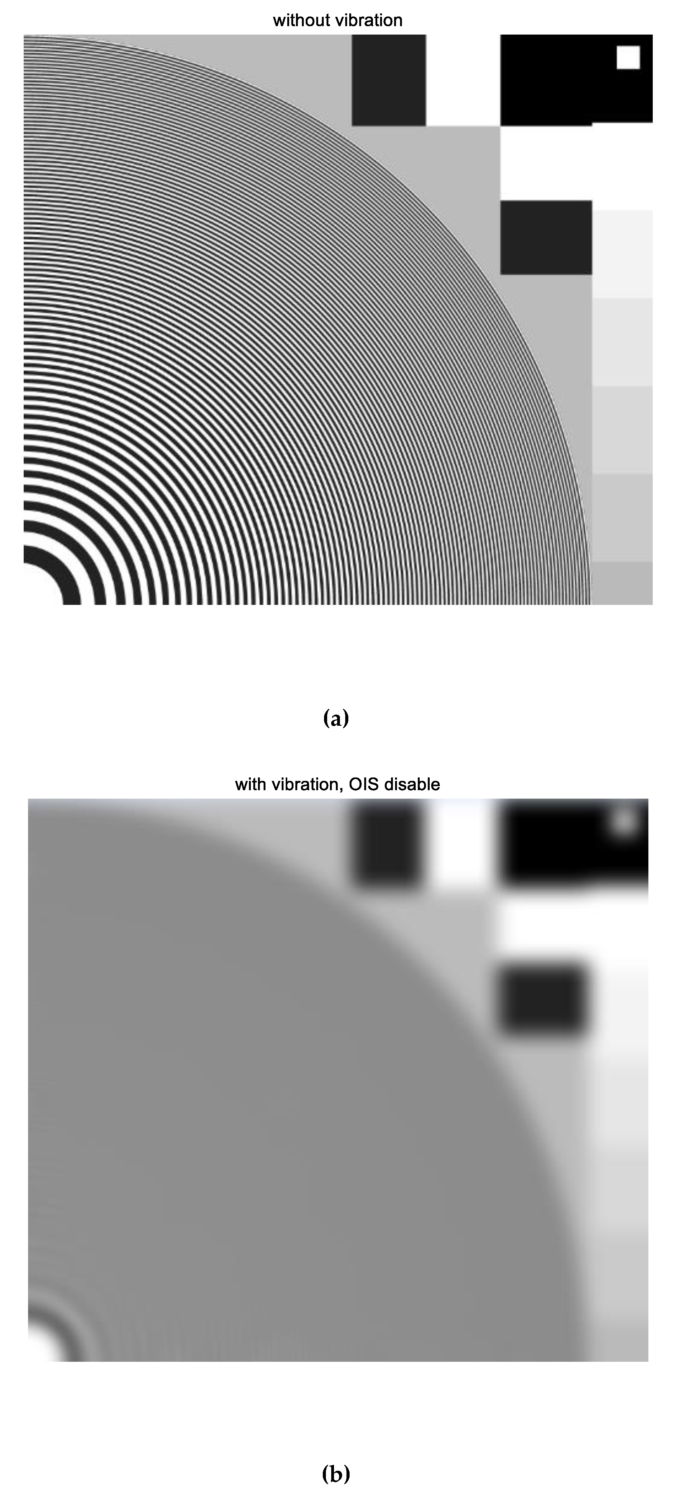
5.2. Image Resolution Test: Qualitative Test

For the image quality test, the proposed controller was applied to ISO 12233 resolution test chart, which is the ISO standard for measuring resolution of electronic still imaging cameras. In this subsection, image quality tests were performed by bare eyes. After zooming Figure 18c,d, similar blurring points were investigated. In the figure, red arrows indicate the similar burring points.

Additionally, as another high resolution test pattern, zone 720 hard edge pattern B was also tested. In the same way, after zooming Figure 19c,d, similar blurring points were searched as well.

In the above qualitative image tests, conventional methods can of course partially compensate image blurring effectively, but the proposed method corrects the image blurring more precisely.

In addition, the proposed method could be applied to reject external vibrations induced from unevenness of the road in automotive application, such as advanced driver assistance systems/autonomous driving (ADAS/AD). In the automotive application, stabilized vision images are crucial to safety of drivers and pedestrians because recognition rate of traffic signs and citizens is highly dependent on image quality [30].

6. Conclusions

This note presents performance limitations of the conventional method, and proposes a new optimal design method for OIS systems. Firstly, performance limitations of the conventional methods were addressed, and secondly a flexible control method was suggested. From the image quality tests, it was verified that the proposed method precisely compensates the influences of the hand vibration. This method is also applicable to low-light shooting (LLS) because exposure time at night should be longer than in daylight, and the longer exposure time is more susceptible to external vibrations. Thus, this method would be effective in robot vision and traffic sign and pedestrian detections in automotive applications.

This note affords three main research results different from the previous results. First, in the conventional control method, performance limitations were presented. And using relation between sensitivity and complementary sensitivity functions, new optimal design without notch filters was proposed. Unlike previous research, phase of the closed loop systems was highlighted, and it was shown that the phase is more important in counteracting systems to external vibrations and disturbances like the OIS system.

References

- Teare, S.W.; Restaino, S.R. Introduction to Image Stabilization; SPIE Press: Bellingham, WA, USA, 2006; Volume 73. [Google Scholar]
- Morimoto, C.; Chellappa, R. Evaluation of image stabilization algorithms. In Proceedings of the 1998 IEEE International Conference on Acoustics, Speech and Signal Processing, Seattle, WA, USA, 15 May 1998; Volume 5, pp. 2789–2792. [Google Scholar]
- Morimoto, C.; Chellappa, R. Fast electronic digital image stabilization. In Proceedings of the 13th International Conference on Pattern Recognition, Vienna, Austria, 25–29 August 1996; Volume 3, pp. 284–288. [Google Scholar]
- Skogestad, S.; Postlethwaite, I. Multivariable Feedback Control: Analysis and Design; Wiley: New York, NY, USA, 1996. [Google Scholar]
- Maciejowski, J.M. Multivariable Feedback Design; Addison-Wesley Publishing Company: Boston, MA, USA, 1989. [Google Scholar]
- Franklin, G.F.; Powel, J.D.; Abbas, E.-N. Feedback Control of Dynamic Systems; Prentice Hall: Upper Saddle River, NJ, USA, 2002. [Google Scholar]
- Pappalardo, C.M.; Guida, D. System identification algorithm for computing the modal parameters of linear mechanical systems. Machines 2018, 6, 12. [Google Scholar] [CrossRef]
- Pappalardo, C.M.; Guida, D. Use of the adjoint method in the optimal control problem for the mechanical vibrations of nonlinear systems. Machines 2018, 6, 19. [Google Scholar] [CrossRef]
- Song, M.-G.; Baek, H.-W.; Park, N.-C.; Park, K.-S.; Yoon, T.; Park, Y.-P.; Li, S.-C. Development of small sized actuator with compliant mechanism for optical image stabilization. IEEE Trans. Magn. 2010, 46, 2369–2372. [Google Scholar] [CrossRef]
- Song, M.-G.; Hur, Y.-J.; Park, N.-C.; Park, K.-S.; Park, Y.-P.; Lim, S.-C.; Park, J.-H. Design of a voice-coil actuator for optical image stabilization based on genetic algorithm. IEEE Trans. Magn. 2009, 45, 4558–4561. [Google Scholar] [CrossRef]
- Sato, K.; Ishizuka, S.; Nikami, A.; Sato, M. Control techniques for optical image stabilizing system. IEEE Trans. Consum. Electron. 1993, 39, 8–10. [Google Scholar] [CrossRef]
- Ertürk, S. Real-time digital image stabilization using Kalman filters. Real-Time Imaging 2002, 8, 317–328. [Google Scholar] [CrossRef]
- Moon, J.-H.; Jung, S.Y. Implementation of an image stabilization system for a small digital camera. IEEE Trans. Consum. Electron. 2008, 54, 206–212. [Google Scholar] [CrossRef]
- Chang, H.J.; Kim, P.J.; Song, D.S.; Choi, J.Y. Optical image stabilizing system using multirate fuzzy PID controller for mobile device camera. IEEE Trans. Consum. Electron. 2009, 55, 303–311. [Google Scholar] [CrossRef]
- Lee, S.K.; K, J.-H. An implementation of closed-loop optical image stabilization system for mobile camera. In Proceedings of the IEEE International Conference on Consumer Electronics 2014, Las Vegas, NV, USA, 10–13 January 2014; pp. 45–46. [Google Scholar]
- Han, X.-F.; Zhang, J.-Y.; Xie, H.-W. Design and simulation of a new miniature camera module using voice coil motor for optical image stabilization. In Proceedings of the International Conference on Mechanical Engineering and Control Automation 2017, Beijing, China, 25–26 March 2017; pp. 345–351. [Google Scholar]
- Skelton, E.; Iwasaki, T.; Grigoriadis, K. A Unified Algebraic Approach to Linear Control Design; Taylor & Francis: New York, NY, USA, 1997. [Google Scholar]
- Boyd, S.; Ghaoui, L.E.; Feron, E.; Balakrishnan, V. Linear Matrix Inequalities in System and Control Theory; SIAM: Philadelphia, PA, USA, 1994. [Google Scholar]
- Suh, S. Unified H∞ control to suppress vertices of plant input and output sensitivity function. IEEE Trans. Control Syst. Technol. 2010, 18, 969–975. [Google Scholar] [CrossRef]
- Crispoltoni, M.; Fravolini, M.L.; Balzano, F.; D’Urso, S.; Napolitano, M.R. Interval fuzzy model for robust aircraft imu sensors fault detection. Sensors 2018, 18, 2488. [Google Scholar] [CrossRef] [PubMed]
- Nguyen, N.P.; Hong, S.K. Sliding Mode Thau Observer for actuator fault diagnosis of quadcopter UAVs. Appl. Sci. 2018, 8, 1893. [Google Scholar] [CrossRef]
- Xie, J.; Wang, L.; Bian, Q.; Zhang, X.; Zeng, D.; Wang, K. Optimal available transfer capability assessment strategy for wind integrated transmission systems considering uncertainty of wind power probability distribution. Energies 2016, 9, 704. [Google Scholar] [CrossRef]
- Jiang, X.; Yin, Z.; Wu, J. Stability analysis of linear systems under time-varying samplings by a non-standard discretization method. Electronics 2018, 7, 278. [Google Scholar] [CrossRef]
- Hong, B.-S.; Wu, M.-H. Online energy management of city cars with multi-objective linear parameter-varying L2-gain control. Energies 2015, 8, 9992–10016. [Google Scholar] [CrossRef]
- Chang, Y.-C.; Chang, H.-C.; Huang, C.-Y. Design and implementation of the permanent magnet synchronous generator drive in wind generation systems. Energies 2018, 11, 1634. [Google Scholar] [CrossRef]
- Ru, P.; Subbarao, K. Nonlinear model predictive control for unmanned aerial vehicles. Aerospace 2017, 4, 31. [Google Scholar] [CrossRef]
- Cheng, C.-K.; Chao, P.C.-P. Trajectory tracking between Josephson junction and classical chaotic system via iterative learning control. Appl. Sci. 2018, 8, 1285. [Google Scholar] [CrossRef]
- Franklin, G.F.; Powell, J.D.; Workman, M.L. Digital Control of Dynamic Systems; Addison-Wesley: Boston, MA, USA, 1990. [Google Scholar]
- Astrom, K.J.; Wittenmark, B. Computer-Controlled Systems Theory and Design, 3rd ed.; Prentice Hall: Englewood Cliffs, NJ, USA, 1997. [Google Scholar]
- Bila, C.; Sivrikaya, F.; Khan, M.A.; Albayrak, S. Vehicles of the future: A survey of research on safety issues. IEEE Trans. Intell. Transp. 2017, 18, 1046–1065. [Google Scholar] [CrossRef]
Figure 1.
Optical image stabilizer systems.
Figure 2.
Step responses with various damping ratios in second order systems.
Figure 3.
Models for optical image stabilization (OIS) systems.
Figure 4.
Frequency responses of conventional controllers.
Figure 5.
Various open loop functions: (a) With lead or pole placement controllers; (b) With PID or lead-lag controllers.
Figure 6.
Relationship between open loop and sensitivity functions.
Figure 7.
Closed loop systems with fictitious vibrations.
Figure 8.
Design specification of .
Figure 9.
Designed optimal controller using Equation (12).
Figure 10.
Frequency responses in conventional control (pole placement method).
Figure 11.
Frequency responses in the proposed method.
Figure 12.
Compared controllers.
Figure 13.
Compared open loop transfer functions.
Figure 14.
Compared sensitivity functions (Gs: dash-dot) and their closed loop systems functions (Gcls: solid).
Figure 15.
Vibration rejection performance (a) at 1 Hz; (b) at 5 Hz; (c) at 10 Hz; (d) at 15 Hz; (e) at 20 Hz.
Figure 16.
Histogram of distance deviations from optical center to actual optical path, Δ.
Figure 17.
Magnitude and phase responses of the closed loop systems.
Figure 18.
(a) Original image; (b) In the presence of vibrations, OIS disabled; (c) In the presence of vibrations, compensated image with the conventional method; (d). In the presence of vibrations, compensated image with the proposed method.
Figure 19.
(a). Original image; (b). In the presence of vibrations, OIS disabled. (c). In the presence of vibrations, compensated image with the conventional method. (d). In the presence of vibrations, compensated image with the proposed method.