Maximum Likelihood-Based Methods for Target Velocity Estimation with Distributed MIMO Radar


1
State Key Laboratory of Millimeter Waves, School of Information Science and Engineering, Southeast University, Nanjing 210096, China
2
School of Electronic and Information, Shanghai Dianji University, Shanghai 201306, China
3
Science and Technology on Electromagnetic Scattering Laboratory, Shanghai 200438, China
*
Author to whom correspondence should be addressed.
†
These authors contributed equally to this work.
Electronics 2018, 7(3), 29; https://doi.org/10.3390/electronics7030029
Submission received: 22 January 2018
/
Revised: 19 February 2018
/
Accepted: 26 February 2018
/
Published: 28 February 2018
Abstract
:The estimation problem for target velocity is addressed in this in the scenario with a distributed multi-input multi-out (MIMO) radar system. A maximum likelihood (ML)-based estimation method is derived with the knowledge of target position. Then, in the scenario without the knowledge of target position, an iterative method is proposed to estimate the target velocity by updating the position information iteratively. Moreover, the Carmér-Rao Lower Bounds (CRLBs) for both scenarios are derived, and the performance degradation of velocity estimation without the position information is also expressed. Simulation results show that the proposed estimation methods can approach the CRLBs, and the velocity estimation performance can be further improved by increasing either the number of radar antennas or the information accuracy of the target position. Furthermore, compared with the existing methods, a better estimation performance can be achieved.
1. Introduction
Usually, the multi-input multi-output (MIMO) radar systems can be classified into the following two types:
In the distributed MIMO radar systems [13,14,15,16], both the spatial and waveform diversities can be adopted to increase the radar performance in target estimation, detection and tracking. Therefore, this paper focuses on the distributed MIMO radar system.
To overcome the challenges brought by the target movement [17,18], the MIMO radar has been adopted to estimate and detect the moving target. For example, the tracking method for the MIMO radar is analyzed in [19]. In [20,21,22], the detection problem for moving target is considered in the scenario with homogeneous and non-homogeneous clutter, respectively. The Bayesian-based method has also been proposed to estimate the position and velocity of moving target in [23,24]. In [25,26,27,28], the fractal-fractional modeling and the Weierstrass-Mandelbrot function have also proposed and can be used to improve the radar performance.
The Carmér-Rao Lower Bound (CRLB) can be used to analyze the target estimation performance in the MIMO radar system. For example, the CRLB for velocity estimation is given in the distributed MIMO radar in [29], but the effect of position estimation error has not been considered. In [30], the CRLB matrix is used to solve the problem of range compression and waveform optimization. Moreover, in [31], the direction finding performance of the MIMO radar is described by the outage CRLB. Different from the existing works, this letter gives the velocity estimation methods for the scenarios with or without the information of target position. Then, the CRLBs are used to measure the velocity estimation performance in the distributed MIMO radar, and the effect of target position error is also considered.
In this paper, the estimation problem for target velocity is addressed in the distributed MIMO radar, and a Maximum Likelihood (ML)-based method is expressed to estimate the target velocity in the scenario with target position information. Then, in the scenario without the position information, an iterative method is proposed to update the target position, and to improve the performance of velocity estimation. Moreover, the corresponding Carmér-Rao Lower Bounds (CRLBs) for both scenarios are derived and compared with the estimation performance of the proposed methods.
Notations: is the norm. stands for a vector with all entries being 1. denotes an identity matrix. denotes the expectation operation. denotes the Gaussian distribution with the mean being and the variance matrix being . ⊗, , and denote the Kronecker product, the trace of a matrix, and the matrix transpose, respectively.
The remainder of this paper is organized as follows. The distributed MIMO radar system is given in Section 2. The estimation method with and without the knowledge of target position are given in in Section 3. Then, the corresponding CRLBs are given in Section 4, and the simulation results are given Section 5. Finally, Section 6 concludes the paper.
2. System Model and Problem Formulation
Different from the colocated MIMO radar system with the close antennas, the distributed MIMO radar system is considered in this paper, where the widely separated antennas are adopted. Additionally, the the transmitters and receivers are also widely separated, as shown in Figure 1. We denote the number of transmitters and receivers as and , respectively. The position of the m-th transmitter () and the n-th receiver () are denoted as and , respectively, where for the 2-dimension measurement or for the 3-dimension measurement.
All the transmitters and receivers are adopted to measure the target velocity . Then, for the signal transmitted by the m-th transmitter and received by the n-th receiver, the Doppler frequency of the received signal can be expressed as
where is denoted as the target position, denotes the wavelength of the transmitted signal, and the direction vectors are defined as
In the radar system, the Doppler frequency is estimated and denoted as , where is the estimation error for the Doppler frequency . Collecting all the estimation errors into a vector
The vector follows the Gaussian distribution with zero-mean, i.e., , where denotes the covariance matrix of the estimation errors. In addition, a vector is also adopted to collect all the estimated Doppler frequencies
And we have
Alternatively, the Doppler frequency vector can be also expressed as
where denotes the direction matrix. Then, (5) can be finally rewritten as
3. Target Velocity Estimation
3.1. With the Target Position Information
When the ML-based method is adopted to estimate the target velocity, the estimated result can be expressed as
where denotes the probability density function (PDF) of the Doppler frequency given the target velocity , and can be expressed as
Therefore, the ML-based estimation method is obtained as
Which is a weighted least square (WLS) problem and can be solved efficiently. Taking the derivative with respect to , the solution of (10) is
3.2. Without the Target Position Information
In the ML-based estimation method (11), the direction matrix is assumed to be known. However, in the practical radar systems, the information of target position is unknown. In this subsection, an iterative method is proposed to estimate the target velocity without the knowledge of target position.
In this scenario, the initially estimated target position is denoted as , and the initially estimated velocity can be obtained from (11) as
where the initial direction matrix is defined as
and are respectively defined as
where
The real target position can be written as
where , and denotes the error of estimated position. Therefore, can be approximated by
And . By defining and as
The Doppler frequency vector can be approximated as
where .
Then, with the estimated target velocity in (12), the estimation of is
which can be solved and simplified as
After obtaining , the target position is updated as (), and used to obtain a new direction matrix . Substitute the updated into (12), and we can iterate the processes from (12) to (24). Finally, the target velocity and position can be obtained as and (), respectively. The details about this algorithm is given in Algorithm 1.
In Algorithm 1, the main complexity lies in the steps to calculate the estimated velocity and position . Therefore, the computational complexity can be roughly calculate as , which depends on the number of transmitters , the number of receivers and the velocity dimension N.
| Algorithm 1 Proposed Algorithm for Estimating Target Velocity | |
| 1: | Input: Doppler frequency vector , initially estimated target position , transmitter positions (), receiver positions (), the number of iterations K. |
| 2: | Initialization: |
| 3: | whiledo |
| 4: | . |
| 5: | . |
| 6: | |
| 7: | . |
| 8: | Update parameters: |
| 9: | end while |
| 10: | Output: the estimated target velocity and the estimated target position . |
4. Carmér-Rao Lower Bound
4.1. With the Target Position Information
The Carmér-Rao Lower Bound (CRLB) of the estimated velocity is defined as
where denotes the Fisher information matrix (FIM) with the i-th row and j-th column entry being
where denotes the i-th column of . Therefore, , and the mean square error (MSE) of the estimated velocity is bounded by the CRLB
4.2. Without the Target Position Information
When the target position is unknown, the Doppler frequency vector and the estimated target position can be respectively rewritten as
where we assume the position error follows the zero-mean Gaussian distribution . By defining , the CRLB of can be expressed as
where the FIM is defined as
Given the target velocity and position , the joint PDF of and is
where
Then, the i-th row and j-th column entry of FIM can be obtained as
Therefore, the following results can be obtained:
- When , we have
- When , we have
Then, the entries of FIM are:
- For the i-row and j-th column of , we have
- For the i-row and j-th column of , we havewhere .
- For the i-row and j-th column of , we have
- For the i-row and j-th column of , we have
Therefore, after simplifications, we have
Using the block matrix method, the inverse of FIM can be obtained as , where we have
Finally, we can obtain the CRLB of target velocity
And the CRLB of target position can be also obtained as
5. Simulation Results
In this section, the simulation results are given, and the simulation parameters are given as follows: the carrier frequency is GHz, the number of dimensions is , and the number of receivers is . The positions of transmitters, receivers and target are shown in Figure 2.
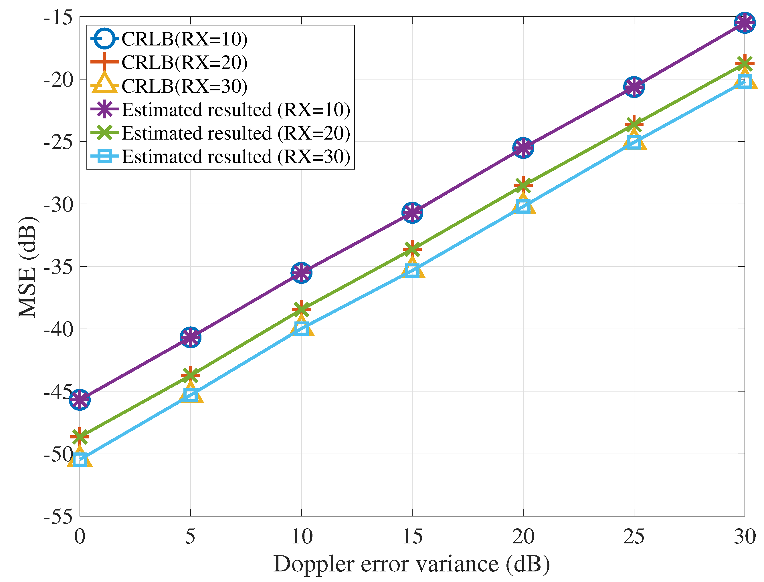
First, with the position information, the estimation performance of target velocity is given in Figure 3. In this figure, both the MSE of ML-based method and CRLB with different Doppler error variances are given, where , and we use to indicate the values of horizontal ordinate. The ML-based estimation method can approach the CRLB, which shows the effective of ML-based method. Additionally, we also give the estimation performance with different numbers of receivers, i.e., , 20 and 30. The estimation performance is improved by increasing the number of receivers.
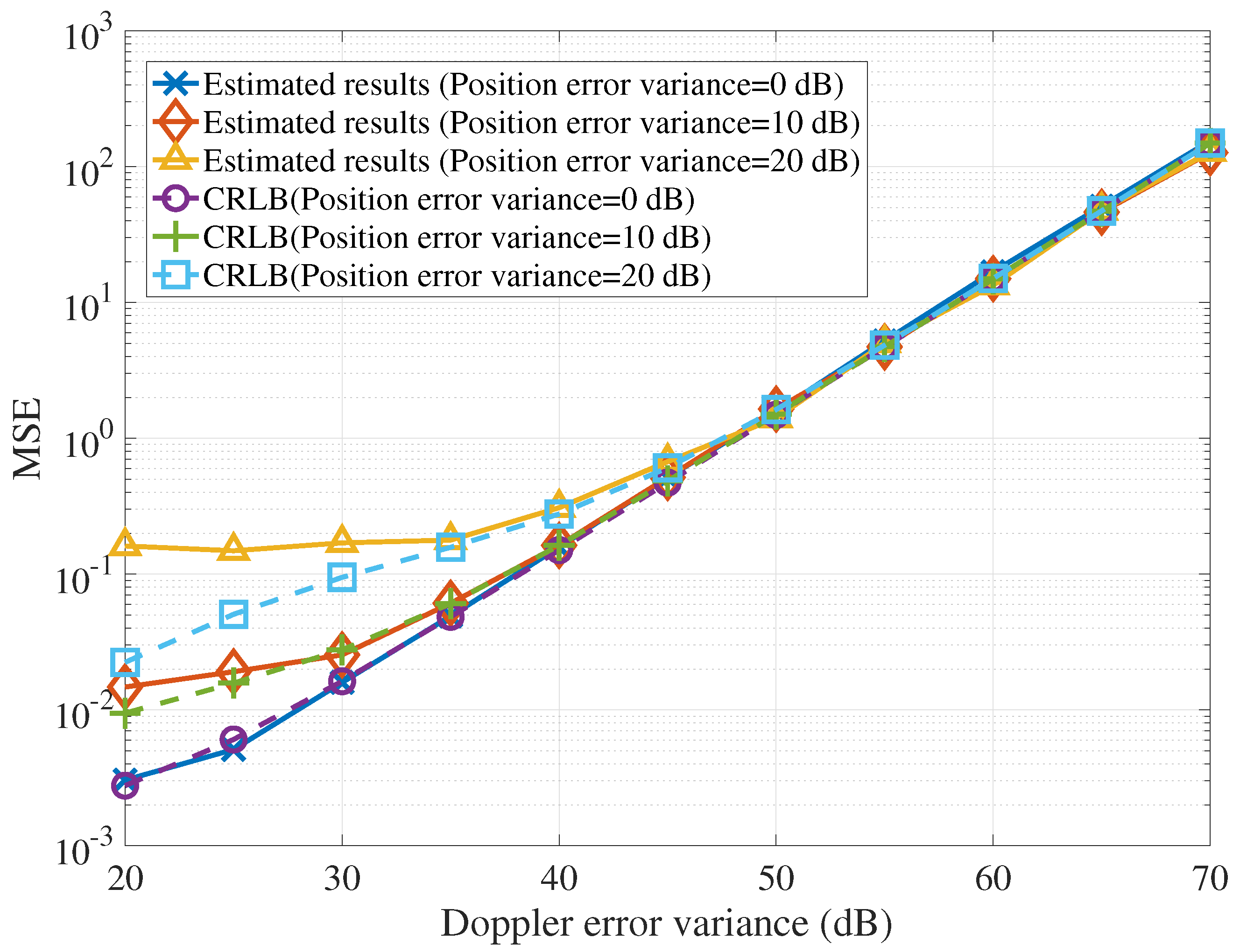
Second, the estimation performance of target velocity with position estimation error is shown in Figure 4, where the number of transmitters and receivers are and , respectively. As shown in this figure, increasing the variance of Doppler error will decrease the estimation performance of target velocity. Additionally, we have , and we use to show the value of in dB. In Figure 4, decreasing the performance of position estimation, i.e., increasing the value of , the performance of velocity estimation is also decreasing, especially, in the scenario with worse performance of position estimation.
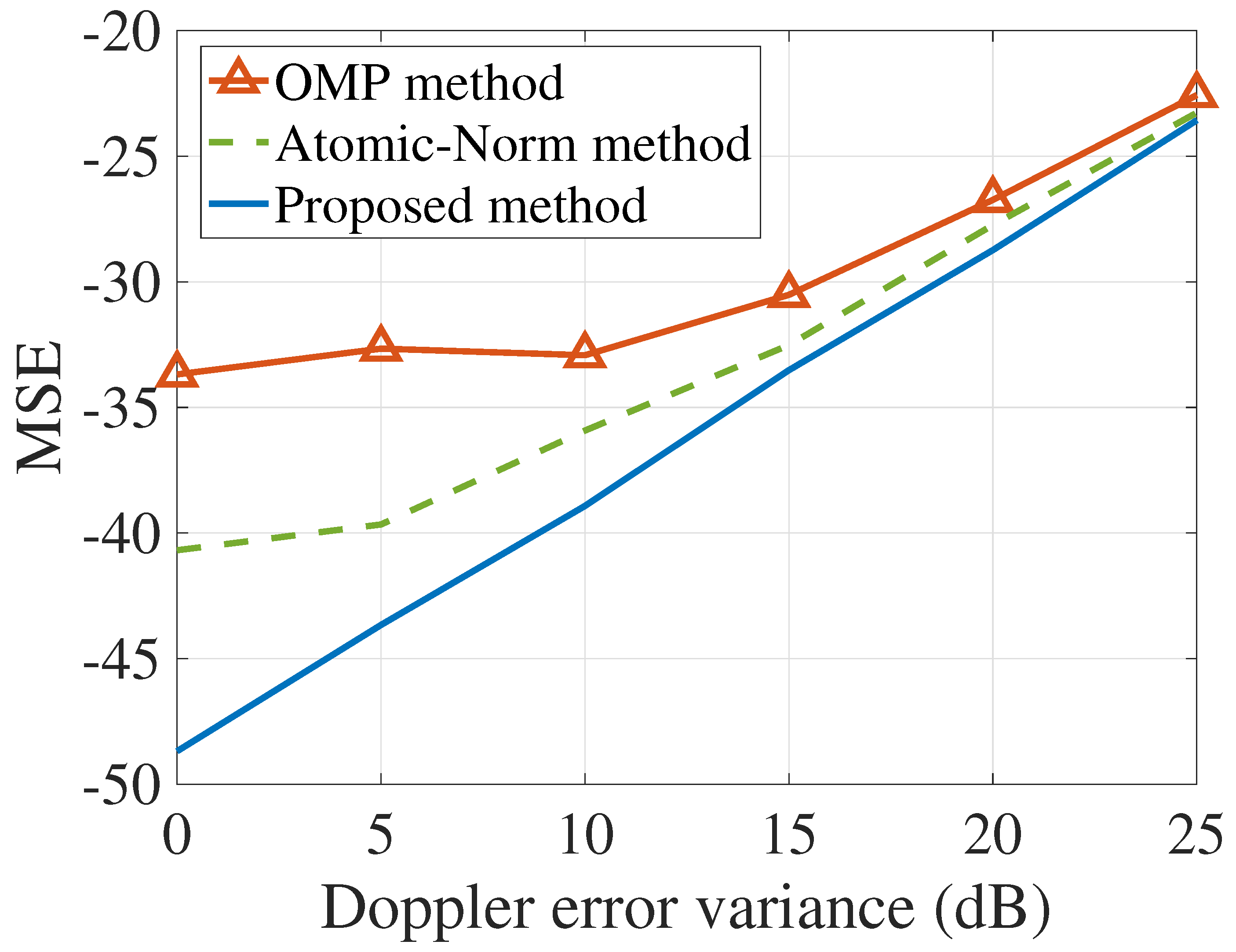
Finally, with the number of RX being 20, we compare the proposed method with the existing methods. As shown in Figure 5, the proposed method is compared with the orthogonal matching pursuit (OMP) method [22] and the Atomic-Norm method [32]. Since both existing methods are based on the theory of compressed sensing, the better performance can be achieved in the scenario with less data. However, in our scenario, we have enough data from the receivers, so the proposed method can achieve better estimation performance. Additionally, since the discretized grids are adopted in the OMP method, when the Doppler variance is good enough, the estimation performance cannot be better with decreasing error of Doppler variance as shown in Figure 5. Therefore, compared with the existing methods, we can achieve the better velocity estimation performance.
6. Conclusions
In the distributed MIMO radar system, the estimation problem for target velocity has been considered in this paper. We have proposed the novel ML-based estimation methods in the scenarios with and without the knowledge of target position to obtain the information of target velocity. Additionally, the corresponding CRLBs have also been derived. Simulation results demonstrate that the proposed estimation methods can approach the CRLBs, and the velocity estimation performance can be further improved by increasing either the number of antennas or the information accuracy about target position. Further work will focus on the estimation of target velocity with the moving radar platforms.
Acknowledgments
This work was supported in part by the National Natural Science Foundation of China (Grant No. 61471117, 61601281, 61501298), and the Open Program of State Key Laboratory of Millimeter Waves (Southeast University).
Author Contributions
Zhenxin Cao and Peng Chen conceived and designed the experiments; Zhimin Chen performed the experiments; Zhenxin Cao and Zhimin Chen analyzed the data; Xinyi He contributed reagents/materials/analysis tools; Peng Chen wrote the paper.
Conflicts of Interest
The authors declare no conflict of interest.
References
- Li, J.; Stoica, P. MIMO radar with colocated antennas. IEEE Signal Process. Mag. 2007, 24, 106–114. [Google Scholar] [CrossRef]
- Davis, M.; Showman, G.; Lanterman, A. Coherent MIMO radar: The phased array and orthogonal waveforms. IEEE Aerosp. Electron. Syst. Mag. 2014, 29, 76–91. [Google Scholar] [CrossRef]
- Liu, W.; Wang, Y.; Liu, J.; Xie, W.; Chen, H.; Gu, W. Adaptive detection without training data in colocated MIMO radar. IEEE Trans. Aerosp. Electron. Syst. 2015, 51, 2469–2479. [Google Scholar] [CrossRef]
- Xu, H.; Blum, R.S.; Wang, J.; Yuan, J. Colocated MIMO radar waveform design for transmit beampattern formation. IEEE Trans. Aerosp. Electron. Syst. 2015, 51, 1558–1568. [Google Scholar] [CrossRef]
- Xu, H.; Wang, J.; Yuan, J.; Shan, X. Colocated MIMO radar transmit beamspace design for randomly present target detection. IEEE Signal Process. Lett. 2015, 22, 828–832. [Google Scholar]
- Haghnegahdar, M.; Imani, S.; Ghorashi, S.A.; Mehrshahi, E. SINR enhancement in colocated MIMO radar using transmit covariance matrix optimization. IEEE Signal Process. Lett. 2017, 24, 339–343. [Google Scholar] [CrossRef]
- Cui, G.; Yu, X.; Carotenuto, V.; Kong, L. Space-time transmit code and receive filter design for colocated MIMO radar. IEEE Trans. Signal Process. 2017, 65, 1116–1129. [Google Scholar] [CrossRef]
- Haimovich, A.M.; Blum, R.S.; Cimini, L.J. MIMO radar with widely separated antennas. IEEE Signal Process. Mag. 2008, 25, 116–129. [Google Scholar] [CrossRef]
- Zheng, L.; Wang, X. Super-resolution delay-Doppler estimation for OFDM passive radar. IEEE Trans. Signal Process. 2017, 65, 2197–2210. [Google Scholar] [CrossRef]
- Park, C.H.; Chang, J.H. Closed-form localization for distributed MIMO radar systems using time delay measurements. IEEE Trans. Wirel. Commun. 2016, 15, 1480–1490. [Google Scholar] [CrossRef]
- Gao, Y.; Li, H.; Himed, B. Knowledge-aided range-spread target detection for distributed MIMO radar in nonhomogeneous environments. IEEE Trans. Signal Process. 2017, 65, 617–627. [Google Scholar] [CrossRef]
- Chen, P.; Qi, C.; Wu, L. Antenna placement optimisation for compressed sensing-based distributed MIMO radar. IET Radar Sonar Navig. 2017, 11, 285–293. [Google Scholar] [CrossRef]
- Fishler, E.; Haimovich, A.; Blum, R.S.; Cimini, L.J.; Chizhik, D.; Valenzuela, R.A. Spatial diversity in radars-models and detection performance. IEEE Trans. Signal Process. 2006, 54, 823–838. [Google Scholar] [CrossRef]
- Fishler, E.; Haimovich, A.; Blum, R.; Chizhik, D.; Cimini, L.; Valenzuela, R. MIMO radar: An idea whose time has come. In Proceedings of the IEEE Radar Conference, Philadelphia, PA, USA, 29 April 2004; pp. 71–78. [Google Scholar]
- Li, J.; Jiang, D.J.; Zhang, X. DOA estimation based on combined unitary ESPRIT for coprime MIMO radar. IEEE Commun. Lett. 2017, 21, 96–99. [Google Scholar] [CrossRef]
- Chen, P.; Wu, L. Coding matrix optimization in cognitive radar system with EBPSK-based MCPC signal. J. Electromagn. Waves Appl. 2015, 29, 1497–1507. [Google Scholar] [CrossRef]
- Dooley, S.R.; Nandi, A.K. Adaptive time delay and Doppler shift estimation for narrowband signals. IEE Proc. Radar Sonar Navig. 1999, 146, 243–250. [Google Scholar] [CrossRef]
- Dogandzic, A.; Nehorai, A. Cramer-Rao bounds for estimating range, velocity, and direction with an active array. IEEE Trans. Signal Process. 2001, 49, 1122–1137. [Google Scholar] [CrossRef]
- Hassanien, A.; Vorobyov, S.A.; Gershman, A.B. Moving target parameters estimation in noncoherent MIMO radar systems. IEEE Trans. Signal Process. 2012, 60, 2354–2361. [Google Scholar] [CrossRef]
- Chen, P.; Qi, C.; Wu, L.; Wang, X. Estimation of extended targets based on compressed sensing in cognitive radar system. IEEE Trans. Veh. Technol. 2017, 66, 941–951. [Google Scholar] [CrossRef]
- He, Q.; Lehmann, N.H.; Blum, R.S.; Haimovich, A.M. MIMO radar moving target detection in homogeneous clutter. IEEE Trans. Aerosp. Electron. Syst. 2010, 46, 1290–1301. [Google Scholar] [CrossRef]
- Chen, P.; Zheng, L.; Wang, X.; Li, H.; Wu, L. Moving target detection using colocated MIMO radar on multiple distributed moving platforms. IEEE Trans. Signal Process. 2017, 65, 4670–4683. [Google Scholar] [CrossRef]
- Jiang, M.; Niu, R.; Blum, R.S. Bayesian target location and velocity estimation for multiple-input multiple-output radar. IET Radar Sonar Navig. 2011, 5, 666–670. [Google Scholar] [CrossRef]
- Chen, P.; Wu, L.; Qi, C. Waveform optimization for target scattering coefficients estimation under detection and peak-to-average power ratio constraints in cognitive radar. Circuits Syst. Signal Process. 2016, 35, 163–184. [Google Scholar] [CrossRef]
- Guariglia, E. Entropy and fractal antennas. Entropy 2016, 18, 1–17. [Google Scholar] [CrossRef]
- Guariglia, E. Fractional derivative of the riemann zeta function. In Fractional Dynamics; Cattani, C., Srivastava, H.M., Yang, X.-J., Eds.; De Gruyter: Berlin, Germany, 2015; pp. 357–368. [Google Scholar]
- Berry, M.V.; Lewis, Z.V. On the Weierstrass-Mandelbrot fractal function. Proc. R. Soc. Lond. Ser. A 1980, 370, 459–484. [Google Scholar] [CrossRef]
- Guariglia, E. Spectral analysis of the Weierstrass-Mandelbrot function. In Proceedings of the 2nd International Multidisciplinary Conference on Computer and Energy Science, Split, Croatia, 12–14 July 2017; pp. 12–14. [Google Scholar]
- He, Q.; Blum, R.S.; Godrich, H.; Haimovich, A.M. Target velocity estimation and antenna placement for MIMO radar with widely separated antennas. IEEE J. Sel. Areas Signal Process. 2010, 4, 79–100. [Google Scholar] [CrossRef]
- Li, L.; Xu, L.; Stoica, P.; Forsythe, K.W.; Bliss, D.W. Range compression and waveform optimization for MIMO radar: A CRB based study. IEEE Trans. Signal Process. 2008, 56, 218–232. [Google Scholar]
- Lehmann, N.; Fishler, E.; Haimovich, A.M.; Blum, R.S.; Cimini, L.; Valenzuela, R. Evaluation of transmit diversity in MIMO radar direction finding. IEEE Trans. Signal Process. 2007, 55, 2215–2225. [Google Scholar] [CrossRef]
- Chu, H.; Zheng, L.; Wang, X. Super-resolution mmWave channel estimation using atomic norm minimization. arXiv, 2018; arXiv:cs.IT/1801.07400. [Google Scholar]
Figure 1.
Velocity measurement using the distributed multi-input multi-output (MIMO) radar.
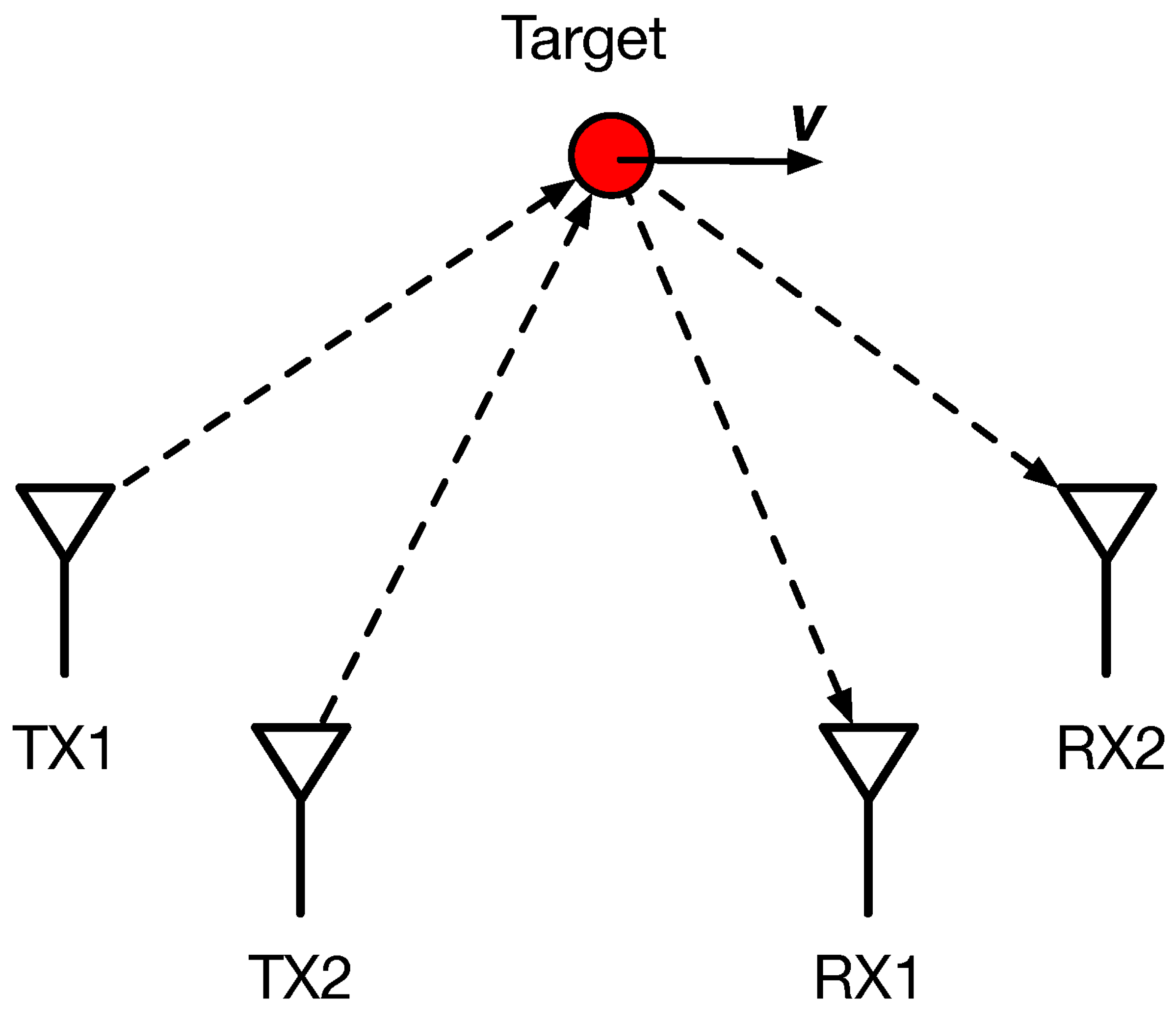
Figure 2.
The positions of transmitters, receivers and target.
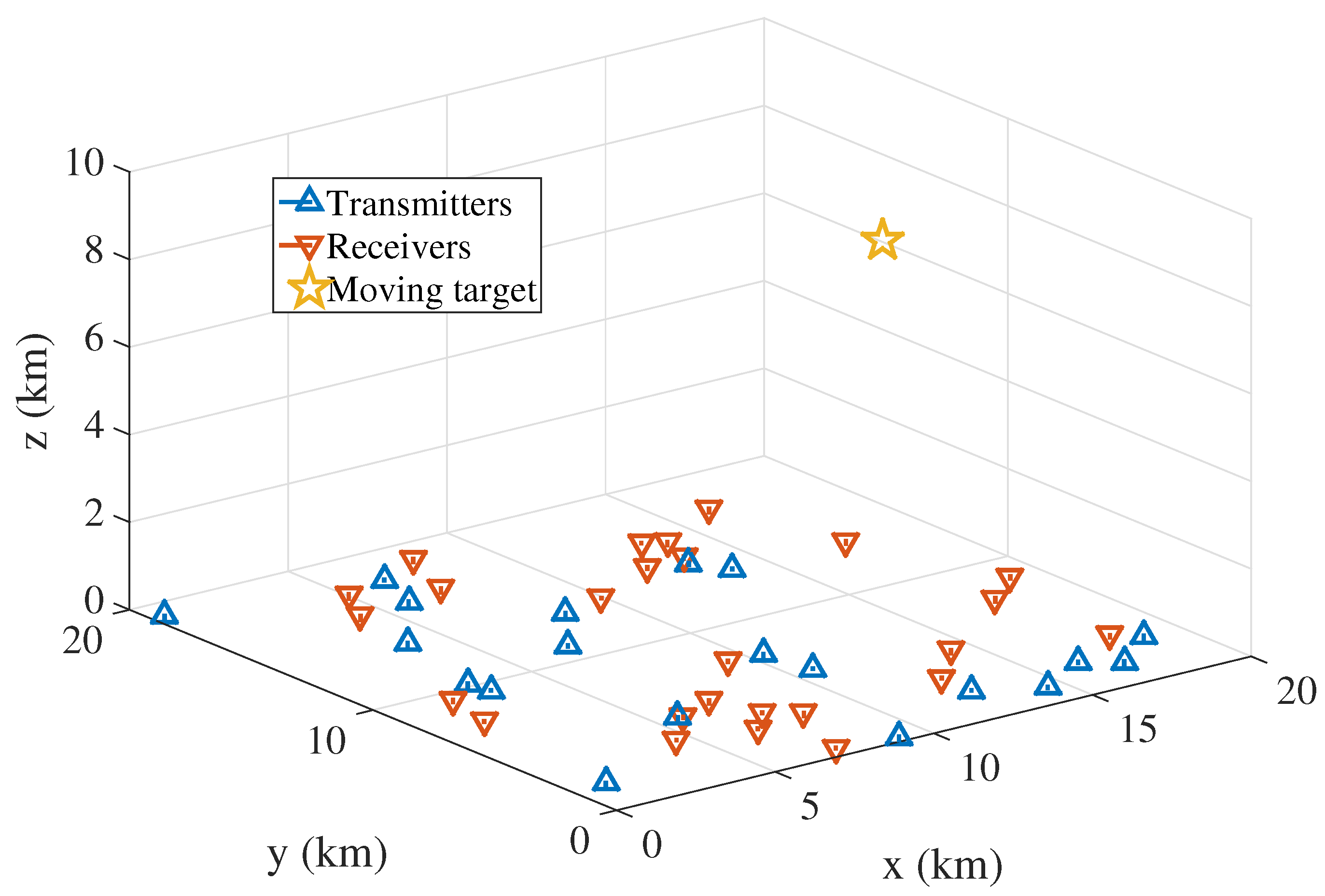
Figure 3.
Target velocity estimation performance without position errors.

Figure 4.
Target velocity estimation performance with position errors.

Figure 5.
Compared with the existing methods.

© 2018 by the authors. Licensee MDPI, Basel, Switzerland. This article is an open access article distributed under the terms and conditions of the Creative Commons Attribution (CC BY) license (http://creativecommons.org/licenses/by/4.0/).
Share and Cite
MDPI and ACS Style
Cao, Z.; Chen, P.; Chen, Z.; He, X. Maximum Likelihood-Based Methods for Target Velocity Estimation with Distributed MIMO Radar. Electronics 2018, 7, 29. https://doi.org/10.3390/electronics7030029
AMA Style
Cao Z, Chen P, Chen Z, He X. Maximum Likelihood-Based Methods for Target Velocity Estimation with Distributed MIMO Radar. Electronics. 2018; 7(3):29. https://doi.org/10.3390/electronics7030029
Chicago/Turabian StyleCao, Zhenxin, Peng Chen, Zhimin Chen, and Xinyi He. 2018. "Maximum Likelihood-Based Methods for Target Velocity Estimation with Distributed MIMO Radar" Electronics 7, no. 3: 29. https://doi.org/10.3390/electronics7030029
Note that from the first issue of 2016, this journal uses article numbers instead of page numbers. See further details here.