Energy-Efficient Scheduling of Periodic Applications on Safety-Critical Time-Triggered Multiprocessor Systems

Abstract

Energy optimization for periodic applications running on safety/time-critical time-triggered multiprocessor systems has been studied recently. An interesting feature of the applications on the systems is that some tasks are strictly periodic while others are non-strictly periodic, i.e., the start time interval between any two successive instances of the same task is not fixed as long as task deadlines can be met. Energy-efficient scheduling of such applications on the systems has, however, been rarely investigated. In this paper, we focus on the problem of static scheduling multiple periodic applications consisting of both strictly and non-strictly periodic tasks on safety/time-critical time-triggered multiprocessor systems for energy minimization. The challenge of the problem is that both strictly and non-strictly periodic tasks must be intelligently addressed in scheduling to optimize energy consumption. We introduce a new practical task model to characterize the unique feature of specific tasks, and formulate the energy-efficient scheduling problem based on the model. Then, an improved Mixed Integer Linear Programming (MILP) method is proposed to obtain the optimal scheduling solution by considering strict and non-strict periodicity of the specific tasks. To decrease the high complexity of MILP, we also develop a heuristic algorithm to efficiently find a high-quality solution in reasonable time. Extensive evaluation results demonstrate the proposed MILP and heuristic methods can on average achieve about 14.21% and 13.76% energy-savings respectively compared with existing work.

1. Introduction

Multiprocessor architecture such as Multi-Processor System-on-Chip (MPSoC) are increasingly believed to be the major solution for an embedded cloud computing system due to high computing power and parallelism. The multiprocessor architecture of an MPSoC incorporates multiprocessors and other functional units in a single case on a single die. Meanwhile, there is an ongoing trend that diverse emerging safety-critical real-time applications, such as automotive, computer vision, data collection and control applications are running simultaneously on the MPSoCs [1]. For these safety-related applications, it is imperative that deadlines should be strongly guaranteed. Due to the strong timing requirements and needed predictability guarantees, real-time cloud computing is a complex problem [2]. To satisfy the timing requirement, task scheduling typically relies on an offline schedule based on the architectures such as TTA (Time Triggered Architecture) such that full predictability is guaranteed [3]. In the computing systems, time-triggered scheduling, where tasks have to be executed at particular points in real time, is often utilized to form a deterministic schedule. To effectively schedule the applications, the safety-critical systems require more elaborated scheduling strategies to meet timing constraints and the precedence relationships between tasks.

Reducing energy consumption or conducting green computing is a critical issue in deploying and operating cloud platforms. When the safety-related applications are executed on MPSoCs, reducing energy consumption is another concern since high energy consumption translates to shorter lifetime, higher maintenance costs, more heat dissipation, lower reliability, and, in turn, has a negative impact on real-time performance. Therefore, this growing demand to accommodate multiple applications running periodically on the safety/time-critical multiprocessor systems necessitates to develop an efficient scheduling approach to fully exploit the energy-saving potential. The high energy consumption mainly comes from the energy consumption at the processor level. To reduce power dissipation of processors, Dynamic Voltage and Frequency Scaling (DVFS) and Power Mode Management (PMM (Note that PMM is also referred to as ‘Dynamic Power Management (DPM)’ [4]. This paper uses the more specific term ‘Power Mode Management’ to avoid any confusion.)) are two well established system-level energy management techniques. DVFS reduces the dynamic power consumption by dynamically adjusting voltage or frequency while PMM explores idle intervals of a processor and switches the processor to a sleep mode to reduce the static power.

Lots of research has been done on scheduling for energy optimization in real-time multiprocessor embedded systems [5,6,7,8,9,10,11]. An application can usually be modeled as a Directed Acyclic Graph (DAG) where nodes denote tasks, and edges represent precedence constraints among tasks. Among these studies, a DAG-based application must be released periodically, whereas tasks in the application can be started aperiodically. In other words, the start time interval between any two consecutive task instances does not need to be fixed to the value of period as long as precedence and deadline constraints can be met. However, such an assumption in these studies is not suitable for the problem of scheduling periodic DAGs on safety/time-critical time-triggered systems. Their solutions in the studies cannot fully guarantee timing predictability and meet the timeliness requirements if the schedulings are not appropriate. Moreover, their methods are merely for single DAG and cannot be directly applied to multiple DAGs.

On the other hand, for a periodic application in time-triggered systems, the scheduling should follow a strictly regular pattern, where besides release time and deadline, the start time of different invocations of a task must be also periodic [12,13,14,15,16,17,18,19,20]. In this case, most research efforts in energy-efficient scheduling on time-triggered multiprocessor systems, which applied mathematical programming techniques such as Integer Linear Programming (ILP), simply and consistently assume that all tasks in the application are strictly periodic [12,13,14,15,16,17,18]. Their time-triggered scheduling approaches are suitable for the tasks that are designed for periodic samplings and actuations.

Nevertheless, tasks within an application are unnecessarily strictly periodic in reality. Today, newly emerging periodic applications may also consist of tasks that do not generate jobs strictly periodically [21]. A typical case can be easily found in the real-world automotive application in engine management system, where most tasks in the application are strictly periodic, and the non-strict periodic tasks are the angle synchronous tasks. Here, for the angle synchronous tasks, the inter-arrival time depend on the revolutions per minute and the number of cylinders of the engine [22,23]. The non-strict periodic tasks are started with relative deadlines corresponding to around an additional 30 degrees of the crankshaft position, after passing a specific rotation of crankshaft position. Therefore, the oversimplified assumption in previous approaches developed for energy-efficient scheduling may impose excessive constraints and degrades scheduling flexibility of the whole system. Furthermore, from the perspective of energy-saving, the excessive constraints result in unnecessary energy consumption. To make readers easy to follow, a motivating example presented in Section 4 will illustrate the problem.

In this paper, we study the energy-efficient scheduling problem arising from the requirements of safety-related real-time applications when deployed in the context of cloud computing embedded platforms. We focus on the problem of static scheduling multiple periodic applications consisting of both strictly and non-strictly periodic tasks on safety/time-critical time-triggered MPSoCs for energy optimization by employing the two powerful techniques: DVFS and PMM. To reduce energy consumption more effectively, both strictly and non-strictly periodic tasks in time-triggered applications should be correctly addressed. This requires an intelligent scheduling that can capture the strict periodicity of specific tasks. Moreover, the problem becomes more challenging when scheduling for energy minimization by combining DVFS with PMM has to consider periodicity of specific tasks in time-triggered systems. In addition, the energy-efficient scheduling problem becomes more complicated as the number of applications running extends from single to multiple. Our main contributions are summarized as the following:

• We consider the unique feature of periodic applications that not all tasks within the applications are strictly periodic in time-triggered systems. A practical task model that can accurately characterize the periodic applications is presented and an energy-efficient scheduling problem based on the model is formulated.
• To solve the problem, we present an improved Mixed Integer Linear Programming (MILP) formulation utilizing the flexibility of non-strictly periodic tasks to reduce unnecessary energy overhead. The MILP method can generate the optimal scheduling solutions.
• To overcome disadvantage of the MILP method when the size of the problem expands, we further develop a heuristic method, named Hybrid List Tabu-Simulated Annealing with Fine-Tune (HLTSA-FT), which integrates the list-based energy-efficient scheduling and tabu-simulated annealing with a fine-tune algorithm. The heuristic can obtain high-quality solutions in a reasonable time.
• We conduct experiments on both synthetic and realistic benchmarks. The experimental results demonstrate the effectiveness of our approach.

It is worth mentioning that, based on the static energy-efficient deterministic schedule (defined in a static configuration file) generated by our proposed methods, the operating system kernel applies it to schedule the partition at its assigned time slot for designing of a practical safety/time-critical partitioned system, where the middleware is integrated to ease interoperability and portability of components to satisfy requirement regarding cost, timeliness, power consumption and so on [24,25].

The remainder of this paper is organized as follows: Section 2 reviews related work in the literature. Section 3 describes models and defines the studied problem. In Section 4, we give a motivating example to explain our idea. Our approach is presented in Section 5. Experimental results are provided in Section 6. The conclusions are presented in Section 7.

2. Related Work

Scheduling for energy optimization is a crucial issue in real-time systems [2,4]. Energy-efficient scheduling of the DAG-based application on the systems have been extensively studied. To name a few, Baskiyar et al. combined DVFS and decisive path scheduling list scheduling algorithm to achieve two objectives of minimizing finish time and energy consumption [6]. Liu et al. distributed the slack time over tasks with the DVFS techniques on the critical path to achieve energy savings [8]. However, they are merely for single DAG-based application. Moreover, these approaches only consider dynamic power consumption, and ignore static power consumption that becomes prominent in the deep submicron domain. In energy-harvesting system, Qiu et al. were devoted to reducing power failures and optimizing the computation and energy efficiency [26], and the authors in [27] addressed the scheduling of implicit deadline periodic tasks on a uniprocessor based on the Earliest Deadline First-As Soon As Possible (EDF-ASAP) algorithm. The works in [28,29] combined DVFS and PMM to minimize energy consumption for scheduling frame-based tasks. However, their approaches can only address independent tasks in a single-processor system. Kanoun et al. proposed a fully self-adaptive energy-efficient online scheduler for general DAG models for multicore DVFS- and PMM-enabled platforms [9]. However, the proposed energy-efficient scheduling solution is designed for soft real-time tasks, where missing deadlines is tolerable.

The aforementioned studies are not applicable for safety-critical applications that have the highest level of safety. Furthermore, in these studies, an application is only periodic in terms of its release time and each task within the application can start aperiodically. Obviously, such an assumption is untenable for a time-triggered application in safety/time-critical systems. The scheduling of tasks in time-triggered systems have also been reported in [13,14,18,19,20]. Lukasiewycz et al. obtained a schedule for time-triggered distributed automotive systems by a modular framework which provided a symbolic representation used by an ILP solver [13]. Sagstetter et al. studied the problem of synthesizing schedules for the static time-triggered segment for asynchronous scheduling in current automotive architectures, and proposed an ILP approach to obtain optimal solutions and a greedy heuristic to obtain high quality solutions [18]. Freier and Chen presented the time-triggered scheduling policies for real-time periodic task model [19]. Gendy introduced techniques to automate the process of searching for a workable schedule and increase the system predictability [20]. Unfortunately, these works only focus on enhancing system performance.

Research efforts devoted to task scheduling for energy optimization in time-triggered embedded systems have received attention recently. Chen et al. presented ILP formulations and developed two algorithms to address the energy-aware task partitioning and processing unit allocation for periodic real-time tasks [15]. However, the work only addresses independent tasks, and it is not suitable for the DAG-based applications. For periodic dependent tasks, Pop et al. proposed a constraint logic programming-based approach for time-triggered scheduling and voltage scaling for low-power and fault-tolerance [16]. Recently, the state-of-the-art work in [17] introduced a key technique to model the idle interval of the cores by means of MILP. The study proposed a time-triggered scheduling approach to minimize total system energy for a given set of applications represented as DAGs and a mapping of the applications. However, the studies all assume that each task and its instances are started in a strictly periodic pattern. In reality, besides the strictly periodic tasks within time-triggered applications, there also exist non-strictly periodic tasks where each instance of a task does not need to be started periodically [21,22,23]. To the best of our knowledge, Ref. [21] is the first study that tried to derive better system performance with scheduling both strictly and non-strictly periodic tasks in the safety-critical time-triggered systems. However, their work only focuses on enhancing schedulability, and energy optimization is not involved. In this paper, we address the energy-efficient scheduling problem for periodic time-triggered applications consisting of both strictly and non-strictly periodic tasks.

Methods for scheduling applications on time-triggered multiprocessor systems are mostly based on mathematical programming techniques [12,13,14,15,16,17,18]. Since scheduling in multiprocessor systems is NP-hard, many heuristics have been developed when the scale of the problem is increased. To schedule multiple DAG-based applications on real-time multiprocessor systems, the studies in [6,8,21,30,31,32,33,34] presented a collection of static greedy scheduling heuristics based on list-based scheduling. The list-based scheduling heuristics are generally accepted and can provide effective scheduling solutions and its performance is comparable with other algorithms at lower time complexity. They efficiently reduce the search space by means of greedy strategies. However, due to the greedy nature, they can only address certain cases efficiently and cannot ensure the solution quality for a broad range of problems.

On the other hand, to explore the solution space for a high-quality solution, current practice in many domains such as job shop scheduling [35], autonomous power systems [36], distributed scheduling [37] and energy-efficient scheduling problems in embedded system [38,39,40], favors Tabu Search (TS)/Simulated Annealing (SA) meta-heuristic algorithms. They have shown superiority to the one-shot list scheduling heuristics, despite a higher computational cost. However, both TS and SA have advantages and disadvantages. In general, the SA algorithm is problem-independent, which is analogous to the physical process of annealing. However, it does not keep track of recently visited solutions and needs more iterations to find the best solution. TS algorithm is more efficient in finding the best solution in a given neighborhood, whereas it cannot guarantee convergence and avoid cycling [35]. Moreover, the algorithms cannot be directly used to solve our problem since the non-strictly periodic tasks in time-triggered applications are ignored (whether a task starts strictly periodic or not has a strong influence on scheduling and total energy consumption of the whole system).

To the best of our knowledge, the heuristic method for our problem is not yet reported. In this paper, we consider to solve the problem by formulating the MILP model to obtain optimal solutions, and further to develop an efficient heuristic algorithm since computation time of the MILP method is intolerable when the problem size increases.

3. Problem Formulation

In this section, we first introduce related models and basic concepts that will be used in the later sections, and then provide the problem formulation. The notations used in this paper and their definitions are listed in

Table 1. Notations.

Symbol	Description
$v_i^m$	Task $v_i$ executed on core m ($1\le m\le M$)
$v_{i,p}^m$	The p-th instance of task $v_i$ executed on core m
$C{v}_{i,j}$	Communication task ($v_i^m$ transfer data to $v_j^n$)
$C_{i,j}$	Communication time between $v_i^m$ and $v_j^n$
$comm(v_i,v_j)$	Communication size between task $v_i$ and $v_j$
$D_k$	Deadline of application $g_k$
$P_k$	Period of application $g_k$
$d_i$	Deadline of task $v_i$
$p_i$	Period of task $v_i$
$H_a$	Hyper-period of all tasks
B	The bus bandwidth
$W_{i,l}^m$	WCET of task $v_i$ on core m under v/f level l
${\chi }^m$	Time overheads for DVFS and task switch on core m
$T_{bet}$	break-even-time
$P_{al}$	Total power when the core is active under v/f level l
$P_{idle}$	Total power when the core is idle
$P_{sleep}$	Total power when the core is sleep
$P_{ba}$	Total Power of when the bus is active
$P_{bi}$	Total power of when the bus is idle
$t_{idle}$	Idle time interval of the core
$t_{sleep}$	Sleep time interval of the core
$E_{cov}$	Total energy overhead of the cores mode switching
$E_{comm}$	Total communication energy consumption in $H_a$
$E_{comp}$	Total computation energy consumption in $H_a$
$E_{total\_H_a}$	Total system energy consumption in $H_a$
$P_{total\_H_a}$	Total power of the MPSoC

.

3.1. System Model

In this paper, we consider a typical MPSoC architecture [17,41,42] shown in Figure 1. The MPSoC architecture consists of M processing cores {core 1, core 2, ..., core M}. Each core has its own local memory, and all cores perform inter-core communication by a high bandwidth shared time-triggered non-preemptive bus to access the main memory. The multi-core platform supports L different voltage or frequency (v/f) levels and a set of total power value {$P_{a1}$, $P_{a2}$, …, $P_{aL}$} ($P_{a1}$>$P_{a2}$>…>$P_{aL}$) corresponding to v/f levels. The bus controller implements a given bus protocol (e.g., time-division multiple access protocol), and assigns bus access rights to individual cores. The communication procedure among inter-core rely on message-passing [30]. The characteristics of the system model are as follows: (1) a DVFS- and PMM-enabled MPSoC; (2) non-preemptive; (3) shared time-triggered bus based on a given protocol; (4) communications are supposed to perform at the same speed without contentions; and (5) each core has independent I/O unit that allows for communication and computation to be performed simultaneously. Note that the real communication cost occurs only in inter-core communications where dependent tasks mapped on different cores. In addition, when the tasks are allocated to the same core, the communication cost becomes zero as the intra-core communication can be ignored.

3.2. Task Model

An application can be modeled by a DAG (or called task graph) comprising a set of dependent nodes connected by edges. This article assumes a periodic real-time task model in which $G=\{g_1,g_2,\dots ,g_K\}$ is a set of K applications to be executed on the MPSoC. Application $g_k\in G$ is denoted as $g_k=\{V_k,E_k,D_k,P_k\}$, where $V_k$ and $E_k$ are set of nodes and edges in $g_k$, respectively, and $D_k$ and $P_k$ are deadline and period of $g_k$, respectively. The deadline $D_k$ is assumed to be a constrained deadline, i.e., it is less than or equal to the period $P_k$. Tasks in $g_k$ share the same period and deadline of $g_k$. We use $H_a$ to describe the least common multiple of the periods of all tasks, which is called the hyper-period. It is well known that scheduling in a hyper-period gives a valid schedule [43].

In a task graph, each node $v_i\in V_k$ denotes a computation task and each edge $e_j\in E_k$ represents a communication task. The computation tasks complete data computation on the processing cores, and the communication tasks assigned to the bus complete data transmission between the cores. Computation and communication tasks can be performed in parallel since the communication operation is non-blocked. The weighted value on the edge indicates the amount of data transferred between connected computation tasks. The worst case execution time (WCET) of a task $v_i$ on a core m under v/f level l is denoted by $W_{i,l}^m$. These profiling information of tasks can be obtained in advance.

On the MPSoC platform, we consider multiple time-triggered applications which are released periodically. As not all tasks within the applications started strictly periodically, we analyze characteristics of the tasks and make a classification of tasks in an application as follows:

• Strictly periodic task: the task in an application should strictly start its instances periodically, which means that the start time interval between two successive task instances is fixed. As a strictly periodic task $v_1$ shows in Figure 2a, in addition to release time and deadline for the application, the start time of different invocations of the task need to also be periodic.
• Non-strictly periodic task: the task in an application need not start its instances periodically, i.e., the start time interval between two successive task instances is not fixed. As a non-strictly periodic task $v_2$ shows in Figure 2b, the start time of different invocations of the task can be aperiodic as long as the deadline of the task can be guaranteed.

In this paper, according to the existence of the non-strictly periodic task, an application is regarded as exactly periodic if all tasks within the application are strictly periodic; otherwise, it is regarded as a loose periodic application.

3.3. Energy Model

Assuming that the MPSoC supports both DVFS and PMM. In this paper, we adopt the same energy model due to its generality and practicality [17,42,44,45]. The total system energy consumption is composed of energy overhead of communication and computation. We assume each processing core has three modes, active, idle and sleep mode, and the shared bus has two modes, active and idle mode. Various practical issues including time and energy overhead of the core mode switching and inter-core communications are also considered in the energy model. We apply inter-task DVFS [5,17,41] technique, where the supply v/f of the core cannot be changed within single task. The dynamic power consumption of a processing core and operation frequency f are given by:

$$P_d=C_{ef}\times V_{dd}\times f,$$

(1)

$$f=k\times {(V_{dd}-V_t)}^2/V_{dd},$$

(2)

where $C_{ef}$ is the effective switching capacitance, $V_{dd}$ is the supply voltage, k is a circuit dependent constant and $V_t$ is the threshold voltage. The static power consumption, $P_s$, is given by:

$$P_s=V_{dd}\times I_{leak},$$

(3)

where $I_{leak}$ denotes leakage current. Therefore, total power consumption when the core is active under v/f level l can be computed as:

$$P_{al}=P_d+P_s+P_{on},$$

(4)

where $P_{on}$ is the intrinsic power that is needed to keep the core on. Thus, the energy consumption of task $v_i^m$ executed on core m at v/f level l can be represented as:

$$E_{al}=W_{i,l}^m\times P_{al}.$$

(5)

When a core does not execute any task (idle mode), its power consumption is primarily determined by the idle power. We assume that $P_{idle}$ and $P_{sleep}$ respectively represent the idle power and sleep power. Normally, we have $P_{idle}>P_{sleep}$. Considering the overhead of switching the processing core between active mode and sleep mode, the definition of break-even time $T_{bet}$ is defined as the minimum time interval for which entering the sleep mode is more effective (energy-wise) when compared to the idle mode, despite of an extra time and energy overhead associated to the mode switch between active mode and sleep mode. In other words, the core should keep in idle mode if the idle interval $t_{idle}<T_{bet}$; otherwise, the core should enter into sleep with power consumption $P_{sleep}$. Similar to [17], $T_{bet}$ can be calculated as:

$$T_{bet}=max\{t_{ms},(E_{ms}-P_{sleep}\times t_{ms})/(P_{idle}-P_{sleep})\},$$

(6)

where $t_{ms}$ and $E_{ms}$ are time and energy overhead of the core mode switching, respectively. The energy consumed in idle mode ($E_{idle}$) and sleep mode ($E_{sleep}$), are calculated respectively as follows:

$$E_{idle}=P_{idle}\times t_{idle},$$

(7)

$$E_{sleep}=P_{sleep}\times t_{sleep}.$$

(8)

Therefore, given a static time-triggered schedule S, the total energy consumption of the processing core is:

$$E_{comp}\left(S\right)=E_{al}\left(S\right)+E_{idle}\left(S\right)+E_{sleep}\left(S\right)+E_{cov}\left(S\right).$$

(9)

The processing core, the bus, and the shared on-chip memory in the architecture complete the data transfer between the two dependent tasks. Specifically, an inter-core communication is issued when two tasks with data dependence are mapped to different processing cores. In addition, the shared on-chip memory stores the intermediate communication. The processing core can initiate a write operation to the shared on-chip memory by providing an address with control information that typically requires one bus clock cycle. The communication time overhead (or latency) refers to the length of time that a message containing multiple words delivered from a source processing core to a target processing core. In the architecture, only one component (e.g., processing core) is allowed to use the bus actively at any one time according to the characteristics of the shared bus. The communication procedure on the shared bus is non-interruptible, thus multiple communications should be serialized. The communication time overhead is proportional to the data transfer size, i.e., $C_{i,j}=comm(v_i,v_j)/B$, where $comm(v_i,v_j)$ is the amount of data transferred between task $v_i$ and task $v_j$, and B is the communication bandwidth [41]. On chip memory will allocate memory space to store intermediate data. The required memory space will be released until the target processing core sends back to the bus controller the successful data transfer. For a task graph, there is no inter-core communication if both the source and the target node of an edge are mapped on the same core. The inter-core communication energy overhead between task $v_i$ and $v_j$ is calculated as $E_{comm}(v_i,v_j)=C_{i,j}\times P_{ba}$, where $P_{ba}$ is the power of active bus.

3.4. Problem Statement

Mapping and scheduling in multiprocessor systems have each been proven to be NP-hard. In this paper, we decouple the problem into mapping and scheduling. It is worth mentioning that we assume the task mapping can be performed by using any algorithms in previous excellent works [10,30,31]. The energy-efficient scheduling problem is defined as illustrated in Figure 3.

Given a DVFS- and PMM-enabled MPSoC shown in Figure 1, multiple periodic applications consisting of both strictly and non-strictly periodic tasks, task mapping and profiling information as inputs, the energy-efficient time-triggered scheduler is to find a static non-preemptive scheduling and a v/f assignment for each task in a hyper-period $H_a$ such that total system energy consumption $E_{total\_H_a}$ is minimized while timing constraints are guaranteed.

4. Motivating Example

For easy understanding, in this section, we first present a motivating example to show that state-of-the-art energy-efficient scheduling on time-triggered systems may not work well on the problem. Assuming that an MPSoC has CORE1 and CORE2, each with a high frequency level $f_H$ and a low frequency level $f_L$. The total active power of the core under $f_H$ and $f_L$ is denoted by $P_{aH}$ and $P_{aL}$. 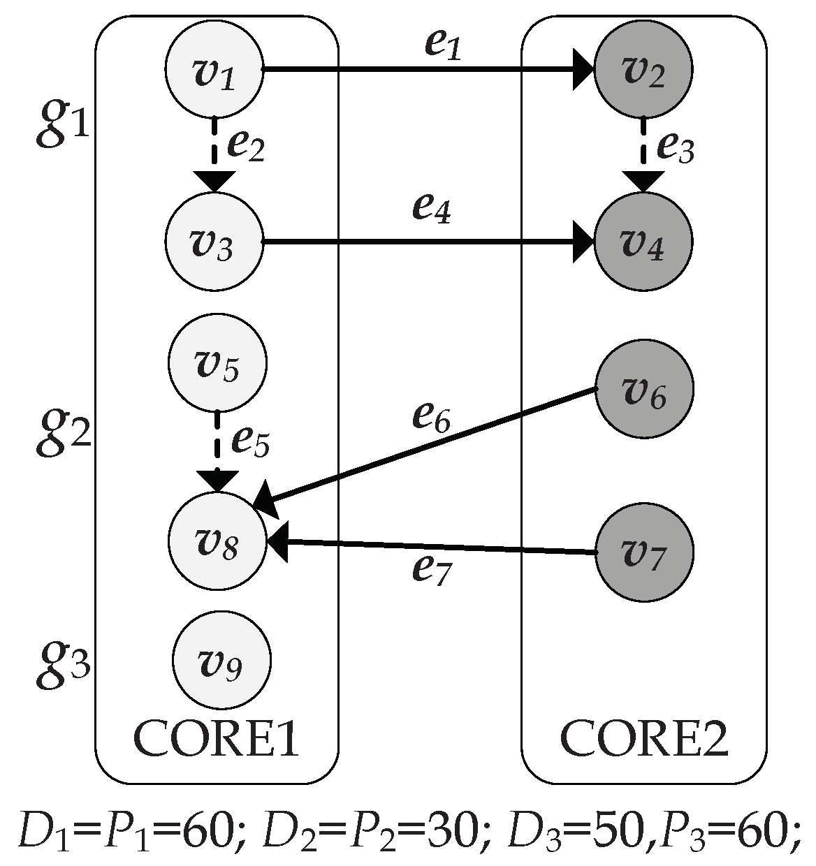Assuming a set of applications (denoted as $g_1$, $g_2$ and $g_3$) and their task mappings on the MPSoC have been given as illustrated in Figure 4. $g_1$ is an exact periodic application in which task $v_1$, $v_2$, $v_3$ and $v_4$ are responsible for collecting data from sensors periodically and $g_2$ is a loose periodic application in which task $v_5$, $v_6$, $v_7$ and $v_8$ are responsible for performing processing data. The edges $e_1$, $e_4$, $e_6$ and $e_7$ indicate their connected tasks are mapped to different cores and the dashed edges $e_2$, $e_3$ and $e_5$ indicate the corresponding tasks are mapped to the same core. Thus, $comm(v_1,v_3)$, $comm(v_2,v_4)$ and $comm(v_5,v_8)$ are equal to 0. The periods for $g_1$, $g_2$ and $g_3$ are 60, 30 and 60, respectively. Task WCETs and power profiles are shown in

Table 2. Task WCETs and power profiles.

${\mathit{v}}_{\mathit{i}}$	WCET(${\mathit{f}}_{\mathit{H}}$)	WCET(${\mathit{f}}_{\mathit{L}}$)	${\mathit{e}}_{\mathit{i}}$	${\mathit{C}}_{\mathit{i},\mathit{j}}$
$v_1$	8	16	$e_1$	8
$v_2$	5	10	$e_2$	4
$v_3$	7	14	$e_3$	5
$v_4$	3	6	$e_4$	5
$v_5$	2	4	$e_5$	6
$v_6$	6	12	$e_6$	3
$v_7$	7	14	$e_7$	9
$v_8$	4	8	-	-
$v_9$	13	26	-	-
$P_{\mathit{aH}}$ = 0.68	$P_{\mathit{aL}}$ = 0.41	$P_{\mathit{idle}}$ = 0.19	$P_{\mathit{ba}}$ = 0.1
$P_{\mathit{sleep}}$ = 0	$P_{\mathit{bi}}$ = 0	$T_{\mathit{bet}}$ = 18	$E_{\mathit{cov}}$ = 0.6

. For simplicity, time unit is 1 ms, power unit is 1 W, and the energy unit is 1 mJ.

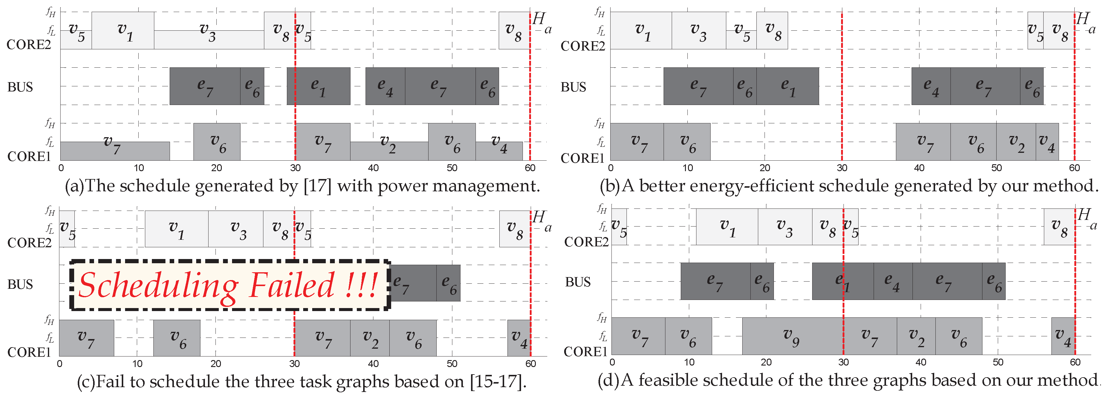
The hyper-period $H_a$ is 60 if we schedule $g_1$ and $g_2$. In one hyper-period, $g_1$ and $g_2$ are released 1 and 2 times, respectively, as well as each task within its application. Based on the assumptions that the start time interval of any two successive instances of a task must be fixed in previous works [15,16,17], the scheduling for energy minimization is shown in Figure 5a. In the schedule, the horizontal axis represents the time, and the heights of task blocks represent the frequency level. The start time interval between two consecutive task instances ($v_{5,2}^2$, $v_{5,1}^2$), ($v_{6,2}^1$, $v_{6,1}^1$), ($v_{7,2}^1$, $v_{7,1}^1$) and ($v_{8,2}^2$, $v_{8,1}^2$) in $g_2$ are equal to 30. The average power consumption in $H_a$ can be calculated as 0.854 W.

In contrast to the scheduling from Figure 5a, the schedule generated by our method in Figure 5b shows a better scheduling for energy-efficiency that the average power consumption in $H_a$ is 0.784 W. In the schedule, the start time interval between task pair ($v_{5,2}^2$, $v_{5,1}^2$), ($v_{6,2}^1$, $v_{6,1}^1$), ($v_{7,2}^1$, $v_{7,1}^1$) and ($v_{8,2}^2$, $v_{8,1}^2$) in $g_2$ do not have such the strict constraint of periodicity, as $g_2$ is a loose periodic application. Due to the flexibility of those non-strictly periodic tasks in the scheduling, increase of total core sleep time and decrease of energy overhead from mode switching can achieve about 8.2% total energy savings compared with Figure 5a.

Assuming that $g_3$ is a exact periodic application in which $v_9$ is responsible for data transformation, we then consider to schedule the three task graphs, $g_1$, $g_2$ and $g_3$. The hyper-period is still 60. We find that scheduling the task graphs based on the simplistic assumptions in [15,16,17] would fail as shown in Figure 5c, as their methods impose overly strict constraints on the task instances within $g_2$. For example, the start time of the two task instances $v_{6,1}^1$ and $v_{6,2}^1$ are 12 and 42, respectively, such that the start time interval between these two task instances is fixed as 30. Thus, $v_9$ cannot be scheduled in a hyper period since the size of $v_6$ is 6 and the size of $v_9$ is 13. However, there actually exists a feasible schedule as shown in Figure 5d. For the non-strictly periodic task $v_6$ in $g_2$, the constraint regarding the periodic interval between the start time of $v_{6,1}^1$ and its next instance $v_{6,2}^1$ is unnecessary. In the schedule, the two task instances, $v_{6,1}^1$ and $v_{6,2}^1$ start at 7 and 42, respectively, and thus $v_9$ can be scheduled at 17.

From the above results, one can observe that the previous studies which do not consider characteristics of non-strictly periodic tasks may result in more energy consumption and even degradation of the schedulability of the whole system. For our problem in this paper, to reduce energy consumption more effectively, a scheduling approach which is aware of the periodicity of specific tasks and utilizes the flexibility of non-strictly periodic tasks is desired.

5. The Proposed Methods

This section presents the energy-efficient scheduling approach jointly with DVFS and PMM techniques for multiple periodic applications consisting of strictly and non-strictly periodic tasks. With consideration of strictness of tasks’ periodicity, we formulate a MILP model to solve the problem and to obtain an optimal scheduling in which the system total energy consumption is the minimum. Then, we develop a heuristic algorithm when the MILP formulation cannot be used to efficiently solve large scale instances.

5.1. MILP Method

ILP-based methods have the advantages of reachable optimality and easy access to various solving tools. We aim to find an energy-efficient time-triggered scheduling and a v/f assignment of all tasks in given an MPSoC, multiple DAGs and task mapping, such that the total system energy consumption is minimized under timing constraints. To obtain optimal energy-efficient scheduling solutions for pre-mapped tasks with consideration of strictness of tasks’ periodicity, we now develop our MILP formulation for the problem based on the practical models defined in Section 3. We build up our MILP formulation step by step, including v/f selection constraints, deadline constraints, periodicity constraints for the strictly periodic tasks, precedence constraints, non-preemption constraints, and an objective function. Firstly, we define the following variables:

• $x_{i,p,l}^m$: binary variable, $x_{i,p,l}^m$ = 1 if v/f level of task $v_{i,p}^m$ is l and $x_{i,p,l}^m$ = 0 otherwise,
• $t{s}_{i,p}^m$: Start time of computation task $v_{i,p}^m,$
• $ct{s}_{i,p;j,q}^{m;n}$: Start time of communication task $C{v}_{i,p;j,q}^{m;n}$ ($v_{i,p}^m$ transfer data to $v_{j,q}^n$),
• $O_{s,p;t,q}^m$: binary variable, $O_{s,p;t,q}^m$ = 1 if task $v_{s,p}^m$ executes before task $v_{t,q}^m$ and $O_{s,p;t,q}^m$ = 0, otherwise.

Then, given task graphs and task mappings, we formulate the MILP model as follows:

Minimize:

$$E_{total\_H_a}=E_{comp}+E_{comm},$$

(10)

Subject to

• Voltage or frequency selection constraints for each task as we use inter-task DVFS:

  $${\Sigma }_{l=1}^L{x}_{i,p,l}^m=1.$$

  (11)
• Deadline constraints (${\chi }^m$ denotes time overheads for DVFS and task switch on core m):

  $$t{s}_{i,p}^m+{\Sigma }_{l=1}^L(x_{i,p,l}^m\times W_{i,l}^m)+{\chi }^m\le d_i.$$

  (12)
• According to strictness of the tasks’s periodicity, we separately determine the start time of these tasks and their instances in $H_a$. Therefore, for the strictly periodic tasks belonging to the time-triggered applications within one hyper-period $H_a$, the periodic constraints can be represented as follows:

  $$t{s}_{i,p+1}^m-t{s}_{i,p}^m=p_i.$$

  (13)
  For any non-strictly periodic task and its instances in $H_a$, the periodic constraint is unnecessary, that is, the interval between the start time of two consecutive instances of the task is no longer fixed as $p_i$.
• Dependency constraints for computation tasks (e.g., source task $v_{i,p}^m$ and target task $v_{k,r}^m$ mapped to the same core:

  $$t{s}_{i,p}^m+{\Sigma }_{l=1}^L(x_{i,p,l}^m\times W_{i,l}^m)+{\chi }^m\le t{s}_{k,r}^m.$$

  (14)
• Dependency constraints for tasks (e.g., source task $v_{i,p}^m$ and target task $v_{j,q}^n$ mapped to different cores.
  (a) $C{v}_{i,p;j,q}^{m;n}$ can be started only after $v_{i,p}^m$ completes:

  $$t{s}_{i,p}^m+{\Sigma }_{l=1}^L(x_{i,p,l}^m\times W_{i,l}^m)+{\chi }^m\le ct{s}_{i,p;j,q}^{m;n},$$

  (15)
  (b) $v_{j,q}^n$ can be started only after $C{v}_{i,p;j,q}^{m;n}$ completes:

  $$ct{s}_{i,p;j,q}^{m;n}+C_{i,j}+{\chi }^m\le t{s}_{j,q}^n.$$

  (16)
• Any two computation task instances mapped to the same core must not overlap in time, as well as the communication tasks in the bus. They can only be executed sequentially. Assume task $v_{s,p}^m$ and task $v_{t,q}^m$ are two task instances, and $MAX$ is a constant far greater than $H_a$. To guarantee either task $v_{t,q}^m$ can run after task $v_{s,p}^m$ finishes, or vice versa, the non-preemption constraint can be expressed as follows:

  $$t{s}_{s,p}^m+{\Sigma }_{l=1}^L(x_{s,p,l}^m\times W_{s,l}^m)+{\chi }^m\le t{s}_{t,q}^m+MAX\times (1-O_{s,p;t,q}^m),$$

  (17)

  $$t{s}_{t,q}^m+{\Sigma }_{l=1}^L(x_{t,p,l}^m\times W_{t,l}^m)+{\chi }^m\le t{s}_{s,p}^m+MAX\times O_{s,p;t,q}^m.$$

  (18)
  The two formulas are also applicable to communication tasks mapped to the bus. The differences between computation and communication tasks are that execution time of computation tasks are variable, while communication time of communication tasks are constant. We can get real computational time of the task on the specified core and real communication cost between the dependent tasks, as task mapping has been given. In addition, communication tasks can be overlapped with the computation tasks independent on them.

To formulate the time interval ($in{t}_i$) of any two adjacent tasks on each core m in one hyper-period $H_a$, we use the interval modelling technique in [17]. The readers interested in the detailed steps of modeling can refer to [17]. Then, according to the definition of $T_{bet}$, for each time interval $in{t}_i$ on the core, we have

$$d_i=\left\{\begin{array}{cc}1,\hfill & \hfill ifin{t}_i\ge T_{bet},\\ 0,\hfill & \hfill ifin{t}_i<T_{bet},\end{array}\right.$$

(19)

where $d_i$ refers to a binary variable in the decision array $darray\left[N\right]$, representing whether the core should remain idle mode $(d_i=0)$ or enter into sleep mode $(d_i=1)$. Assuming there are N tasks on the core in $H_a$, the total idle and sleep interval ($t_{idle}$ and $t_{sleep}$) can be represented as follows:

$$t_{idle}={\Sigma }_{1\le i\le N}((1-d_i)\times in{t}_i),$$

(20)

$$t_{sleep}={\Sigma }_{1\le i\le N}(d_i\times in{t}_i).$$

(21)

The total energy overheads of mode switch for the core can be calculated as follows:

$$E_{cov}={\Sigma }_{1\le i\le N}(d_i\times E_{ms}).$$

(22)

Note that the step function introduced by $d_i$ in Equation (19) and the multiplication of $in{t}_i$ and binary variable $d_i$ in Equations (20) and (21) are nonlinear equations. Such problems can be solved by commercial or open-source ILP solvers after linearization. Solutions to similar problems have been presented in [46]. We now present the linearization process for our problem.

To linearize the multiplication of $d_i\times in{t}_i$, we define a new variable $r_i$, such that $r_i=d_i\times in{t}_i$. It is obvious that $in{t}_i\le H_a$. The multiplication can be linearized as the following constraints:

$$r_i-in{t}_i\le 0,$$

(23)

$$r_i-d_i\times H_a\le 0,$$

(24)

$$in{t}_i-r_i+d_i\times H_a\le H_a.$$

(25)

The step function introduced by $d_i$ in Equation (19) can be transformed to the following constraint:

$$d_i\times (in{t}_i-T_{bet})+(1-d_i)\times (T_{bet}-in{t}_i)\ge 0.$$

(26)

In Equation (26), the multiplication of $d_i\times in{t}_i$ are linearized by using Equations (23)–(25).

Based on these formulations, lastly, we can obtain an optimal scheduling and minimum overall energy consumption $E_{total\_H_a}$ by solving the MILP model with ILP solver.

Limitation of the MILP-based method: Though we can obtain an optimal solution by solving the MILP formulation with modern ILP solvers, it is time-consuming to search the optimal solution for our problem. Specifically, to construct time interval for each task instance in one hyper-period, the time interval modeling in the previously discussed MILP-based method particularly yields a large number of variables, and results in dramatically increased exploration space. The problem may even not be solved because of memory overflow when input size of tasks to be scheduled is large. To address this, we propose an efficient heuristic algorithm to reduce the exponentially increasing scale in Section 5.2.

5.2. Heuristic Algorithm

In this section, we develop a heuristic algorithm, named Hybrid List Tabu-Simulated Annealing with Fine-Tune (HLTSA-FT). Different from the TS/SA algorithm mentioned in Section 2, the proposed algorithm has the following innovations: (1) the HLTSA-FT integrates list scheduling with TS/SA to take advantage of both algorithms and to mitigate their adverse effects. Based on our problem, the decomposition and solution process is iteratively guided by the HLTSA-FT algorithm that employs the proper intensification and diversification mechanism. In HLTSA-FT, the SA supplemented with a tabu list can reduce the number of revisiting old solutions and cover a broader range of solutions; (2) list-based scheduling performed in the List-based and Periodicity-aware Energy-efficient Scheduling (LPES) function can efficiently obtain feasible solutions for our problem; (3) in addition, solutions can be further improved by applying problem specific and heuristic information to guide the process of optimization. Specifically, a fine-tune phase performed in the $FT$ function is presented to make minor adjustments of the accepted solution to find a better solution more rapidly. Therefore, the total number of iterations can be reduced and solution quality can be improved. The details of HLTSA-FT are given in Algorithm 1. Three main steps in the algorithm are:

Initialization. The step (in Lines 1–3) first sets appropriate parameters including the initial temperature $T_0$, the maximum number of iterations $LPMAX$, the maximum number of consecutive rejections $RMAX$, the cooling factor $\delta$ and the maximum length of the tabu list $TL$. Then, the algorithm builds $TL$ with length of $TLIST\_LEN$, and sets aspiration criterion A. The $initial\_solution\_gen\left(\right)$ function generates an initial solution ${\lambda }_0$ (v/f assignment for each task instance in $H_a$) as the starting point of optimization process. Since a good initial solution can accelerate the convergence process, the function integrates the MILP model of a relaxed formulation (e.g., by neglecting the idle and sleep interval formulations). ${\lambda }_0$ is evaluated and the current optimal energy consumption is denoted as $E_{cur}$. The aspiration criterion accepts the move provided that its total energy is lower than that of the best solution found so far. It helps with restricting the search from being trapped at a solution surrounded by tabu neighbors. The tabu list stores recently visited solutions and helps saving considerable computation time by avoiding revisits.

Iteration. In each iteration (in Lines 5–26), the $solution\_neighbor\left(\right)$ function (Line 5) generates neighborhood ${\lambda }_{new}$ by applying a small perturbation (swap move) to current solution ${\lambda }_{cur}$. In our context, v/f assignments for the tasks are in a neighbourhood. ${\lambda }_{new}$ is generated in two steps: (i) select two tasks; and (ii) swap their v/f levels. Then, ${\lambda }_{new}$ is checked for feasibility (i.e., if constraints mentioned above are met) by $solution\_feasible$ function. If the solution is not in the tabu list or satisfies the aspiration criterion, it is selected. Otherwise, a new solution is regenerated. Then, the solution is translated to an energy-efficient schedule by using the $LPES$ function (Line 6). The solution ${\lambda }_{new}$ which consumes less energy will always be accepted, and when ${\lambda }_{new}$ is an inferior solution, it may still be accepted with a probability $Pro(\Delta E,T)=exp(-\Delta /T)$ where T is the annealing temperature at current iteration. This transition probability can help the algorithm to escape from local optima. Once accepted, ${\lambda }_{new}$ is put in the tabu list $TL$ and the current solution is updated by replacing ${\lambda }_{cur}$ with ${\lambda }_{new}$ for next iteration. Then, the FT phase (Line 16) will performed to fine-tune the accepted ${\lambda }_{new}$. Otherwise, the solution ${\lambda }_{new}$ is discarded with $rjnum$ plus 1. The algorithm then decreases the temperature and continues to the next iteration.

Algorithm 1: The HLTSA-FT Heuristic Algorithm

Stopping Criteria. The search procedure will be stopped if the number of iterations or the variable $rjnum$ reaches the predefined value. The variable $rjnum$ stores the current number of continuous rejections, and it represents that no superior solution exists in the neighborhood and the search has reached a near optimal solution once $rjnum$ reaches $RMAX$.

In the next two subsections, we give a detailed description of the $LPES$ and $FT$.

5.2.1. LPES

To obtain a feasible scheduling for energy reduction efficiently, the scheduling for our problem needs to addresses two aspects. First, a priority assignment (i.e., execution order of tasks) must satisfy the corresponding constraints (including deadline and precedence constraints for each task graph, and periodicity constraints for the strictly periodic tasks) in the schedule, and maximize the total interval available for energy management. Second, the intervals need to be allocated efficiently to reduce energy consumption. In this paper, we apply the List-based and Periodicity-aware Energy-efficient Scheduling (LPES) method. The first aspect is addressed through bottom level (b-level) based priority assignment. The second aspect is addressed through a modified simple MILP model whose number of variables is only linear with the number of tasks.

List scheduling is a type of scheduling heuristics in which ready tasks are assigned priorities and ordered in a descending order of priority. A ready task is a task whose predecessors have finished executing. Each time, the task with the highest priority is selected for scheduling. If more than one task has the same priority, ties are broken using the strategy such as the random selection method. Priority assignment based on the b-level has been adopted in energy-aware multiprocessor scheduling. The b-level of a task is defined as the length of the longest path from the beginning of the task to the bottom of the task graph. As we focus on multi-DAGs in our problem, we define the b-level of task $v_{i,p}^m$ and its next instance $v_{i,p+1}^m$ within $H_a$ as:

$$BL(v_{i,p}^m)=BL(v_{i,p+1}^m)+p_i.$$

(27)

We calculate b-level values of all tasks and their instances, and sort them in a list which is ordered in descending order. The higher the value of b-level, the higher the priority of the task. An example is shown as below:

Example 1.

Consider the case given in the form of two task graphs $g_1$ and $g_2$ in Figure 4. The b-level of tasks in $H_a$ are shown in

Table 3. The b-level of each task in one hyper-period.

Tasks	$v_{1,1}^2$	$v_{2,1}^1$	$v_{3,1}^2$	$v_{4,1}^1$	$v_{5,1}^2$	$v_{6,1}^1$	$v_{7,1}^1$	$v_{8,1}^2$	$v_{5,2}^2$	$v_{6,2}^1$	$v_{7,2}^1$	$v_{8,2}^2$
b-level	29	13	15	3	42	43	50	34	12	13	20	4

. Thus, execution order of tasks on CORE1 and CORE2 are denoted as {$v_{7,1}^1\to v_{6,1}^1\to v_{7,2}^1\to v_{2,1}^1\to v_{6,2}^1\to v_{4,1}^1$} and {$v_{5,1}^2\to v_{8,1}^2\to v_{1,1}^2\to v_{3,1}^2\to v_{5,2}^2\to v_{8,2}^2$}, respectively.

Based on the given priority and v/f assignment for each task, a scheduling with PMM should be generated to reduce total energy consumption. The time interval can be directly modeled as the following:

Assuming that there are N task instances on a core m in a hyper-period $H_a$, all these tasks are stored in a task list represented as $T_1,T_2,\dots ,T_i,\dots ,T_N(1\le i\le N)$ where tasks are ordered in descending order of their priorities. As the tasks in the first hyper-period shown in Figure 6, the time interval between any two adjacent tasks, $T_i$ and $T_{i+1}(1\le i\le N-1)$, can be directly calculated as:

$$in{t}_i=st\left(T_{i+1}\right)-ft\left(T_i\right),$$

(28)

where $st\left(T_i\right)$ and $ft\left(T_i\right)$ denote start time and finish time of task $T_i$, respectively. As we focus on task scheduling in one hyper-period and task execution are repeated in each hyper-period, there are N time intervals. The last time interval $in{t}_N$ between task $T_1$ and task $T_N$ is calculated as $in{t}_N=[H_a-ft\left(T_N\right)]+[st\left(T_1\right)-0]$.

In the time interval modeling in Section 5.1, a large number of intermediate integer variables are used to check timing information of every task instance to determine the closest task instance for a task instance. While compared with the time interval modeling in [17], the number of constraints and many decision variables (e.g., $x_{i,p,l}^m$ and $O_{s,p;t,q}^m$,) and the intermediate variables (e.g., $A_{s,p;t,q}^m$, $B_{s,p;t,q}^m$, and $O_{s,p;t,q}^m-B_{s,p;t,q}^m$ in [17]) have been greatly reduced. After obtaining each idle time $in{t}_i$, we use the ILP solver to obtain an energy-efficient scheduling.

5.2.2. FT

To find solutions that can further reduce energy consumption, a fine-grained adjustment of the neighborhood range is performed for the accepted solution (line 16 in Algorithm 1). We now present the details of FT phase. The core idea of FT is to increase the potential energy savings by tuning priorities that still satisfy corresponding constraints of task graphs (not blindly or randomly adjusting priorities). In this study, for the strictly periodic tasks, their priorities remain unchanged since the strictness of periodicity of task start time limits the possibility of adjustment within a hyper-period. The non-strictly periodic task instances in $H_a$ do not have to follow the strict condition that all tasks need to be started periodically; thus, they have space for execution-order adjustment. On the other hand, the tasks that have the same b-level value (tie-breaking tasks) also have chances to adjust their priorities. We focus on these tasks that may have better schedule flexibility and, correspondingly, make full use of it to achieve more energy savings. The pseudo-code of the FT is listed in Algorithm 2.

Algorithm 2: The FT Algorithm

In Algorithm 2, firstly, the priority assignments of tasks on each core are recorded according to the accepted solution ${\lambda }_{new}$. Then, the FT keeps strictly periodic tasks unchanged. For tie-breaking and non-strictly periodic tasks, it adjusts and records their priorities in possible priority assignment array $pos\_priority\left[\right]$ by using $priority\_adj\left(\right)$ function. Next, for each element in $pos\_priority\left[\right]$, the algorithm performs $LPES$. In each iteration, the feasible solution ${\lambda }_{fine}$ (checked for feasibility by $solution\_feasible$ function) that can reduce the energy consumption is stored. Finally, the tasks are adjusted iteratively until no improvement can be achieved. Note that FT can be used directly in the optimization process to find an optimal solution quickly if the initial solution is good. The FT scheme is illustrated through the following example.

Example 2.

In Example 1, the initial execution order of tasks on CORE1 and CORE2 are {$v_{7,1}^1\to v_{6,1}^1\to v_{7,2}^1\to v_{2,1}^1\to v_{6,2}^1\to v_{4,1}^1$} and {$v_{5,1}^2\to v_{8,1}^2\to v_{1,1}^2\to v_{3,1}^2\to v_{5,2}^2\to v_{8,2}^2$}, respectively. Among them, task $v_{2,1}^1$ and task $v_{6,2}^1$ are tie breaking tasks, and tasks belonging to application $g_2$ are non-strictly periodic. Thus, they can be adjusted (swapped) as long as the precedence constraints are guaranteed. The corresponding schedule after FT can be seen in Figure 5b, execution order of tasks on CORE1 and CORE2 are {$v_{7,1}^1\to v_{6,1}^1\to v_{7,2}^1\to v_{6,2}^1\to v_{2,1}^1\to v_{4,1}^1$} and {$v_{1,1}^2\to v_{3,1}^2\to v_{5,1}^2\to v_{8,1}^2\to v_{5,2}^2\to v_{8,2}^2$}, respectively. The improvement of power consumption on the system after FT is, therefore, 8.2%.

6. Experiment Evaluation

This section presents the experimental setup and case studies. To evaluate and demonstrate the efficiency of our proposed approaches, the experiments are performed on a 3.60 GHz 4-core PC with 4 GB of memory under Windows 7. The same 70 nm technology power parameters of the processor are used as in the studies [17,42,44,45]. Code is written in C language, and we use the IBM ILOG CPLEX 12.5.0.0 Solver to solve the MILP formulations. In each case, CPLEX is given a time limit of 10 h.

6.1. Experiment Setup

Our experiments include 12 applications represented by task graph TG1–TG12. TG1–TG3 are based on industrial, automotive, and consumer applications [47]. TG4–TG6 are three applications from ‘Standard Task Graph’ [48], which are based on real applications, namely, a robotic control application, the FPPPP SPEC benchmark and a sparse matrix solver. In addition, we use a general randomized task-graph generator TGFF [49] to create six different periodic applications (TG7–TG12) with typical industrial characteristics in our experiments. These task graphs are from the original example input file (e.g., kbasic, kseries-paralle and robtst) that come from the software package. Then, we consider nine combinations (i.e., five relatively small benchmarks, namely SG1–SG5, and four large benchmarks, namely LG1–LG4) of these task graphs from TG1–TG12. Each benchmark has 2–5 task graphs with features including different topologies (such as chain, in-tree, out-tree, and fork-join), different lengths of critical paths and numbers of dependent tasks. The period of the task graphs are distributed randomly in [10, 2000] ms. We define a parameter $\alpha$ varied from [0, 1] for the whole set of tasks in each benchmark, which reflects the ratio between the strictly and non-strictly periodic tasks. In other words, all tasks are strictly periodic if $\alpha$ is equal to 1, and non-strictly periodic if $\alpha$ is equal 0.

We consider a 4-core architecture for our experiment. The power model is based on a typical 70 nm technology processor, which has been applied in the works [17,41,42,44,45]. The accuracy of the processor power model has been verified by SPICE simulation. For fairness of comparison, parameters of cores power, voltage levels and energy overhead of processor mode switch are referred to [17]. As shown in

Table 4. Core power model parameters.

$\mathit{Level}$	1	2	3	4	5
${\mathit{V}}_{\mathit{dd}}$ (V)	0.85	0.8	0.75	0.7	0.65
$\mathit{f}$ (GHz)	2.10	1.81	1.53	1.26	1.01
${\mathit{P}}_{\mathit{d}}$ (mW)	655.5	489.9	370.4	266.7	184.9
${\mathit{P}}_{\mathit{s}}$ (mW)	462.7	397.6	340.3	290.1	246
	$P_{idle}$ = 276 mW;	$P_{sleep}$ = 0.08 mW;	$E_{ms}$ = 0.385 mJ

, the processor can operate at five voltage levels within the range of 0.65 V to 0.85 V with 50 mV steps and the corresponding frequencies vary from 1.01 GHz to 2.10 GHz. The corresponding dynamic power $P_d$ and static power $P_s$ under different v/f level are calculated according to the energy model in Section 3.3 and the technology constants (e.g., $C_{ef}$, k, and $V_t$) from [42,44,45]. The time overhead of processor mode switch $t_{ms}$ and voltage/frequency switch are 10 ms and 600 $\mu$s, respectively, from [50]. For the mapping step, we use the task assignment algorithm in [31] to assign each task to the MPSoC.

6.2. Experiment Results

This section presents the evaluation of our improved MILP method in Section 5.1 and heuristic algorithm in Section 5.2. The number of tasks and edges of each benchmark is shown in first column of

Table 5. Average power consumption under different methods.

Benchmarks (Tasks/Edges)	Power Consumption (W)
	SMILP	IMILP			HLTSA-FT
	$\forall \mathit{\alpha }$	$\mathit{\alpha }=3/4$	$\mathit{\alpha }=1/2$	$\mathit{\alpha }=1/4$	$\mathit{\alpha }=3/4$	$\mathit{\alpha }=1/2$	$\mathit{\alpha }=1/4$
SG1 (13/15)	2.71	2.49	2.32	2.15	2.49	2.33	2.15
SG2 (19/16)	2.96	2.61	2.39	2.14	2.63	2.39	2.17
SG3 (22/12)	2.73	2.57	2.42	2.21	2.58	2.45	2.24
SG4 (25/31)	2.98	2.74	2.55	2.48	2.76	2.56	2.49
SG5 (34/23)	4.11	3.78	3.60	3.49	3.82	3.63	3.51
Average Reduction	-	8.38%	14.38%	19.86%	7.92%	13.88%	19.48%
		14.21%			13.76%
LG1 (108/72)	TL	TL	TL	TL	3.93	3.41	3.37
LG2 (230/241)	TL	TL	TL	TL	4.89	4.26	3.79
LG3 (355/329)	TL	TL	TL	TL	4.77	4.39	3.55
LG4 (416/263)	TL	TL	TL	TL	4.11	3.70	3.14

.

6.2.1. Evaluation of the Improved MILP

We evaluate and compare our improved MILP method (represented by IMILP) with existing scheduling method (denoted as SMILP) in which the periodic constraint must be strictly followed in the start of all tasks [17]. Table 5 shows average power consumptions in one hyper-period (i.e., the average value of $E_{total\_H_a}$ divided by $H_a$) under different MILP-based methods. The results are obtained in three different cases with the factor $\alpha$ varying from 1/4 to 3/4 with step size 1/4.

From Table 5, one can see that SMILP fails to increase energy savings in contrast to our IMILP. Compared with SMILP, the IMILP in case $\alpha$ = 3/4, 1/2 and 1/4 reduces power consumption for small benchmarks SG1-SG5 by, 8.38%, 14.38% and 19.86%, respectively. The average power consumption can be reduced by 14.21%. The results demonstrate that the simplistic assumption in previous SMILP methods where each task and its task instances must strictly start periodically can lead to an increase in energy consumption. On the other hand, column “SMILP” under “Power Consumption (W)” illustrates the power consumption under SMILP in any cases of $\alpha$ remain unchanged. However, the results under IMILP (from column 3–5 and 6–8) show that the smaller value of $\alpha$, the more power consumption can be reduced. This is because our IMILP can capture the periodicity of specific tasks belonging to their applications, and deals with strictly and non-strictly periodic tasks correctly. To exploit energy-savings, the IMILP method effectively utilizes the flexibility of non-strictly periodic tasks in scheduling as the tasks do not need to start periodically.

6.2.2. Evaluation of the HLTSA-FT

We first compare HLTSA-FT heuristic method with MILP-based methods. The average power consumptions under different $\alpha$ are listed in the last three columns in Table 5. Compared with SMILP, the HLTSA-FT in case $\alpha$ = 3/4, 1/2 and 1/4 reduces power consumption for small benchmarks SG1–SG5 by 7.92%, 13.88% and 19.48%, respectively. The power consumption can be reduced on average, by 13.76%. For the five test cases, the average (minimum) deviation of the HLTSA-FT from the IMILP is only 3.2% (1.9%). The result demonstrates our HLTSA-FT heuristic can find near optimal solutions and its performance is close to that of IMILP for SG1–SG5. Although the MILP method can obtain optimal results, the computation time of the method grows exponentially with increasing size of benchmarks as shown in columns 2–4 in

Table 6. Average computation time under different methods for various $\alpha$.

Benchmarks	IMILP			LSA			HLTSA			HLTSA-FT
	$\mathit{\alpha }=3/4$	$\mathit{\alpha }=1/2$	$\mathit{\alpha }=1/4$	$\mathit{\alpha }=3/4$	$\mathit{\alpha }=1/2$	$\mathit{\alpha }=1/4$	$\mathit{\alpha }=3/4$	$\mathit{\alpha }=1/2$	$\mathit{\alpha }=1/4$	$\mathit{\alpha }=3/4$	$\mathit{\alpha }=1/2$	$\mathit{\alpha }=1/4$
SG1	8.115	8.856	12.838	4.634	4.851	5.193	0.983	1.137	1.602	1.204	1.252	2.37
SG2	12.306	18.974	21.244	4.315	9.183	15.589	4.902	5.926	10.39	4.991	6.878	9.649
SG3	22.928	32.730	96.795	20.059	28.308	31.443	7.998	10.341	30.464	8.656	9.908	32.004
SG4	65.983	97.253	112.581	39.229	50.943	112.556	15.831	16.955	28.77	18.534	18.775	27.639
SG5	624.600	1839.851	2603.3	178.315	205.233	255.689	27.041	27.541	51.837	27.426	28.53	55.51
LG1	TL	TL	TL	846.9	2899.5	5220.98	504.94	1022.7	2455.3	632.06	1349.56	1904.56
LG2	TL	TL	TL	594.88	4534.12	10,120.82	123.18	2611.54	2956.88	318.8	3286.26	4294.3
LG3	TL	TL	TL	3695.8	24,170.1	34,201.16	920.36	2329.4	3645.92	849.62	2361.98	3283.77
LG4	TL	TL	TL	9639.8	23,339.78	35,815.02	2858.25	2903.53	5439.96	3553.46	4513.72	6601.95

. The sign ‘TL’ in Table 5 and Table 6 indicates that the MILP methods for LG1–LG4 cannot generate any optimal solution in limited time (10 h in our experiment). This verifies that the ILP solver fails to find the optimal solutions for models with large instances. However, our HLTSA-FT heuristic algorithm can always generate feasible solutions efficiently for the large benchmarks LG1–LG4. Thus, HLTSA-FT provides a good way for designers to search for energy-efficient scheduling when computation time is intolerable.

We then compare HLTSA-FT with existing heuristic algorithms [38,39,40]. As mentioned in Section 2, the SA-based algorithms have been widely applied to achieve near-optimal solutions for low power scheduling. For fair comparison, we modify and implement the energy-efficient scheduling methods for our problem under three configurations: LSA, HLTSA, and HLTSA-FT. The LSA heuristic applies the list-based SA algorithm but does not consider tabu list and fine-tune phase. The HLTSA heuristic considers LSA integrating tabu list but no fine-tune phase. We evaluate and compare our HLTSA-FT algorithm with these heuristics in terms of two performance metrics: (1) the solution quality and (2) the computation time of searching process.

One can see that the HLTSA and HLTSA-FT outperform LSA in solution quality. The comparison of average power consumption of HLTSA-FT with those of SA-based algorithms are presented in Figure 7 and Figure 8, respectively. In Figure 7, for small benchmarks SG1–SG5, the HLTSA and HLTSA-FT reduce average power consumption by 4.41% and 13.31%, respectively, compared with LSA. In Figure 8, for large benchmarks LG1–LG4, the HLTSA and HLTSA-FT reduce average power consumption by 6.09% and 19.27%, respectively, compared with LSA. This is due to the fact that HLTSA and HLTSA-FT use short-term memory of recently visited solutions known as tabu list in SA to escape from local optima. The search can be restricted from retiring to a previously visited solution and performance of SA can be enhanced significantly with help of the tabu list.

Moreover, our HLTSA-FT improves the solution quality in contrast to HLTSA. In Figure 7, for small benchmarks SG1–SG5, the HLTSA-FT in case $\alpha$ = 3/4, 1/2 and 1/4 reduces average power consumption by 8.79%, 8.91% and 10.11%, respectively, compared with HLTSA. In Figure 8, for large benchmarks LG1-LG4, the HLTSA-FT in case $\alpha$ = 3/4, 1/2 and 1/4 reduces average power consumption by 9.37%, 13.32% and 19.61%, respectively, compared with HLTSA. The reason lies in the fact that the performance is significantly improved by introducing the FT phase. The HLTSA without FT phase focuses on searching for better (concerning energy) solutions blindly and randomly, a lot of which are however abandoned because of violation of corresponding precedence and deadline constraints. The HLTSA-FT actively looks around for near solutions and leads the way to potential energy-efficient schedules by adjusting execution order of tasks if the precedence and deadline constraints are satisfied.

The column 5–13 in Table 6 presents average computation time under different SA-based methods for various $\alpha$. The comparison results are obtained over 10 runs when solving our problem. As can be seen from the table, an interesting observation is that the computation time increases as $\alpha$ decreases. This is caused by the fact that, as $\alpha$ decreases, the number of constraints for specific strictly periodic tasks decreases and the search space of the problem becomes larger. This just demonstrates that our problem requires an effective heuristic algorithm to reduce complexity when the input size becomes larger.

HLTSA and HLTSA-FT outperform LSA on the convergence speed. For example, compared with LSA for different benchmarks (SG1–SG5, LG1–LG4), the HLTSA algorithm under $\alpha$ = 1/2 reduces the average computation time by 76.6%, 35.5%, 63.5%, 66.7%, 86.6%, 64.7%, 42.4%, 90.4%, and 87.6%, respectively, and the HLTSA-FT algorithm under $\alpha$ = 1/2 reduces the average computation time by 74.2%, 25.1%, 65.0%, 63.1%, 86.1%, 53.5%, 27.5%, 90.2% and 80.7%, respectively. This is because LSA does not keep track of recently visited solutions and needs more iterations to find the best solution, while HLTSA and HLTSA-FT exploit the beauty of tabu search and simulated annealing to ensure the convergence at faster rate. Furthermore, one can observe that our HLTSA-FT algorithm can improve the solution quality (in Figure 7 and Figure 8), without increasing significantly the number of required simulations compared with the HLTSA (in Table 6).

To summarize, the experimental results presented above show that the proposed HLTSA-FT heuristic algorithm achieves a good trade-off between solution quality and solution generation time compared with the IMILP, LSA and HLTSA methods as the problem scale becomes larger. The algorithm is a scalable heuristic method that users can adjust the configuration parameters of the algorithm according to the specific input. To achieve further performance improvement, the HLTSA-FT algorithm can obtain high-quality solutions by increasing optimization iterations or executing multiple times within an acceptable time.

7. Conclusions

This paper has investigated the problem of scheduling a set of periodic applications for energy optimization on safety/time-critical time-triggered systems. In the applications, besides strictly periodic tasks, there also exist non-strictly periodic tasks in which different invocations of a task can start aperiodically. We present a practical task model to characterize the strictness of the task’s periodicity, and formulate a novel scheduling problem for energy optimization based on the model. To address the problem, we first propose an improved MILP model to obtain energy-efficient scheduling. Although the MILP method can generate optimal solutions, its solution computation time grows exponentially with the number of inputs. Therefore, we further develop an HLTSA-FT algorithm to reduce complexity and efficiently obtain a high-quality solution within a reasonable time. Extensive evaluations on both synthetic and realistic benchmarks have demonstrated the effectiveness of our improved MILP method and the HLTSA-FT algorithm, compared with the existing studies.

Some issues are taken into account in our future work. In this paper, we assume that task mappings are given as a fixed input. For a higher energy efficiency, mapping and scheduling on time-triggered multiprocessor systems need to be integrated since they are inter-dependent. Currently, we are working on solving this problem. Furthermore, we intend to study how to integrate our approaches with online scheduling methods on the realistic safety/time-critical multiprocessor systems to leverage system-wide energy consumption.

References

1. Kang, S.H.; Kang, D.; Yang, H.; Ha, S. Real-time co-scheduling of multiple dataflow graphs on multi-processor systems. In Proceedings of the 2016 Design Automation Conference, Austin, TX, USA, 5–9 June 2016; pp. 1–6. [Google Scholar]
2. García-Valls, M.; Cucinotta, T.; Lu, C. Challenges in real-time virtualization and predictable cloud computing. J. Syst. Archit. 2014, 60, 726–740. [Google Scholar] [CrossRef]
3. Kopetz, H. The Time-Triggered Model of Computation. In Proceedings of the IEEE Real-Time Systems Symposium, Madrid, Spain, 4 December 1998; Volume 2, pp. 168–177. [Google Scholar]
4. Mittal, S. A Survey of Techniques for Improving Energy Efficiency in Embedded Computing Systems. Int. J. Comput. Aided Eng. Technol. 2014, 6, 440–459. [Google Scholar] [CrossRef]
5. Zhang, Y.; Hu, X.; Chen, D.Z. Task Scheduling and Voltage Selection for Energy Minimization. In Proceedings of the Design Automation Conference, New Orleans, LA, USA, 10–14 June 2002; pp. 183–188. [Google Scholar]
6. Baskiyar, S.; Abdel-Kader, R. Energy aware DAG scheduling on heterogeneous systems. Cluster Comput. 2010, 13, 373–383. [Google Scholar] [CrossRef]
7. Luo, J.; Jha, N.K. Static and Dynamic Variable Voltage Scheduling Algorithms for Real-Time Heterogeneous Distributed Embedded Systems. In Proceedings of the IEEE International Conference on VLSI Design, Bangalore, India, 11 January 2002; p. 719. [Google Scholar]
8. Liu, Y.; Veeravalli, B.; Viswanathan, S. Novel critical-path based low-energy scheduling algorithms for heterogeneous multiprocessor real-time embedded systems. In Proceedings of the International Conference on Parallel and Distributed Systems, Hsinchu, Taiwan, 5–7 December 2007; pp. 1–8. [Google Scholar]
9. Kanoun, K.; Mastronarde, N.; Atienza, D.; Van der Schaar, M. Online Energy-Efficient Task-Graph Scheduling for Multicore Platforms. IEEE Trans. Comput.-Aided Des. Integr. Circuits Syst. 2014, 33, 1194–1207. [Google Scholar] [CrossRef] [Green Version]
10. Kianzad, V.; Bhattacharyya, S.S.; Qu, G. CASPER: An Integrated Energy-Driven Approach for Task Graph Scheduling on Distributed Embedded Systems. In Proceedings of the IEEE International Conference on Application-Specific Systems, Architecture Processors, Samos, Greece, 23–25 July 2005; pp. 191–197. [Google Scholar] [Green Version]
11. Zhou, J.; Yan, J.; Cao, K.; Tan, Y.; Wei, T.; Chen, M.; Zhang, G.; Chen, X.; Hu, S. Thermal-Aware Correlated Two-Level Scheduling of Real-Time Tasks with Reduced Processor Energy on Heterogeneous MPSoCs. J. Syst. Archit. 2017, 82, 1–11. [Google Scholar] [CrossRef]
12. Davare, A.; Zhu, Q.; Natale, M.D.; Pinello, C.; Kanajan, S.; Vincentelli, A.S. Period optimization for hard real-time distributed automotive systems. In Proceeding of the 44th annual Design Automation Conference, San Diego, CA, USA, 4–8 June 2007; pp. 278–283. [Google Scholar]
13. Lukasiewycz, M.; Schneider, R.; Goswami, D.; Chakraborty, S. Modular scheduling of distributed heterogeneous time-triggered automotive systems. In Proceeding of the Design Automation Conference, Sydney, NSW, Australia, 30 January–2 February 2012; pp. 665–670. [Google Scholar]
14. Balogh, A.; Pataricza, A.; Rácz, J. Scheduling of Embedded Time-triggered Systems. In Proceedings of the 2007 Workshop on Engineering Fault Tolerant Systems (EFTS ’07), Dubrovnik, Croatia, 4 September 2007; ACM: New York, NY, USA, 2007. [Google Scholar]
15. Chen, J.J.; Schranzhofer, A.; Thiele, L. Energy minimization for periodic real-time tasks on heterogeneous processing units. In Proceedings of the IEEE International Symposium on Parallel & Distributed Processing, Rome, Italy, 23–29 May 2009; pp. 1–12. [Google Scholar]
16. Pop, P. Scheduling and voltage scaling for energy/reliability trade-offs in fault-tolerant time-triggered embedded systems. In Proceedings of the IEEE/ACM International Conference on Hardware/Software Codesign and System Synthesis, Salzburg, Austria, 30 September–3 October 2007; pp. 233–238. [Google Scholar]
17. Chen, G.; Huang, K.; Knoll, A. Energy optimization for real-time multiprocessor system-on-chip with optimal DVFS and DPM combination. ACM Trans. Embed. Comput. Syst. 2014, 13, 111. [Google Scholar] [CrossRef]
18. Sagstetter, F.; Lukasiewycz, M.; Chakraborty, S. Generalized Asynchronous Time-Triggered Scheduling for FlexRay. IEEE Trans. Comput.-Aided Des. Integr. Circuits Syst. 2017, 36, 214–226. [Google Scholar] [CrossRef]
19. Freier, M.; Chen, J.J. Time Triggered Scheduling Analysis for Real-Time Applications on Multicore Platforms. In Proceedings of the RTSS Workshop on REACTION, Rome, Italy, 2–5 December 2014; pp. 43–52. [Google Scholar]
20. Gendy, A.K.G. Techniques for Scheduling Time-Triggered Resource-Constrained Embedded Systems. Ph.D. Thesis, University of Leicester, Leicester, UK, 2009. [Google Scholar]
21. Hu, M.; Luo, J.; Wang, Y.; Veeravalli, B. Scheduling periodic task graphs for safety-critical time-triggered avionic systems. IEEE Trans. Aerosp. Electron. Syst. 2015, 51, 2294–2304. [Google Scholar] [CrossRef]
22. Freier, M.; Chen, J.J. Sporadic Task Handling in Time-Triggered Systems. In Proceedings of the International Workshop on Software and Compilers for Embedded Systems, Sankt Goar, Germany, 23–25 May 2016; pp. 135–144. [Google Scholar]
23. Kramer, S.; Ziegenbein, D.; Hamann, A. Real world automotive benchmark for free. In Proceedings of the International Workshop on Analysis Tools and Methodologies for Embedded and Real-Time Systems, Lund, Sweden, 7 July 2015. [Google Scholar]
24. García-Valls, M.; Domínguez-Poblete, J.; Touahria, I.E.; Lu, C. Integration of Data Distribution Service and distributed partitioned systems. J. Syst. Archit. 2017, 83, 23–31. [Google Scholar] [CrossRef]
25. García-Valls, M.; Calva-Urrego, C. Improving service time with a multicore aware middleware. In Proceedings of the Symposium on Applied Computing, Marrakech, Morocco, 3–7 April 2017; pp. 1548–1553. [Google Scholar]
26. Qiu, K.; Gong, Z.; Zhou, D.; Chen, W.; Xu, Y.; Shi, X.; Liu, Y. Efficient Energy Management by Exploiting Retention State for Self-powered Nonvolatile Processors. J. Syst. Archit. 2018, 87, 22–35. [Google Scholar] [CrossRef]
27. Ghadaksaz, E.; Safari, S. Storage Capacity for EDF-ASAP Algorithm in Energy-Harvesting Systems with Periodic Implicit Deadline Hard Real-Time Tasks. J. Syst. Archit. 2018. [Google Scholar] [CrossRef]
28. Devadas, V.; Aydin, H. On the Interplay of Voltage/Frequency Scaling and Device Power Management for Frame-Based Real-Time Embedded Applications. IEEE Trans. Comput 2011, 61, 31–44. [Google Scholar] [CrossRef]
29. Gerards, M.E.T.; Kuper, J. Optimal DPM and DVFS for Frame-based Real-time Systems. ACM Trans. Archit. Code Optim. 2013, 9, 41. [Google Scholar] [CrossRef]
30. Kwok, Y.K.; Ahmad, I. Static scheduling algorithms for allocating directed task graphs to multiprocessors. ACM Comput. Surv. 1999, 31, 406–471. [Google Scholar] [CrossRef] [Green Version]
31. Schmitz, M.; Al-Hashimi, B.; Eles, P. Energy-Efficient Mapping and Scheduling for DVS Enabled Distributed Embedded Systems. In Proceedings of the Conference on Design, Automation and Test in Europe (DATE ’02), Paris, France, 4–8 March 2002; pp. 514–521. [Google Scholar]
32. Guzek, M.; Pecero, J.E.; Dorronsoro, B.; Bouvry, P. Multi-objective evolutionary algorithms for energy-aware scheduling on distributed computing systems. Appl. Soft Comput. J. 2014, 24, 432–446. [Google Scholar] [CrossRef] [Green Version]
33. Xie, G.; Zeng, G.; Liu, L.; Li, R.; Li, K. Mixed real-time scheduling of multiple DAGs-based applications on heterogeneous multi-core processors. Microprocess. Microsyst. 2016, 47, 93–103. [Google Scholar] [CrossRef]
34. Xie, G.; Zeng, G.; Liu, L.; Li, R.; Li, K. High performance real-time scheduling of multiple mixed-criticality functions in heterogeneous distributed embedded systems. J. Syst. Archit. 2016, 70, 3–14. [Google Scholar] [CrossRef]
35. Zhang, C.Y.; Li, P.G.; Rao, Y.Q.; Guan, Z.L. A very fast TS/SA algorithm for the job shop scheduling problem. Comput. Oper. Res. 2008, 35, 282–294. [Google Scholar] [CrossRef]
36. Katsigiannis, Y.A.; Georgilakis, P.S.; Karapidakis, E.S. Hybrid Simulated Annealing-Tabu Search Method for Optimal Sizing of Autonomous Power Systems With Renewables. IEEE Trans. Sustain. Energy 2012, 3, 330–338. [Google Scholar] [CrossRef]
37. Chan, F.T.; Prakash, A.; Ma, H.; Wong, C. A hybrid Tabu sample-sort simulated annealing approach for solving distributed scheduling problem. Int. J. Prod. Res. 2013, 51, 2602–2619. [Google Scholar] [CrossRef]
38. He, D.; Mueller, W. A Heuristic Energy-Aware Approach for Hard Real-Time Systems on Multi-core Platforms. In Proceedings of the Euromicro Conference on Digital System Design, Izmir, Turkey, 5–8 September 2012; pp. 288–295. [Google Scholar]
39. Luo, J.; Jha, N.K. Power-Efficient Scheduling for Heterogeneous Distributed Real-Time Embedded Systems. IEEE Trans. Comput.-Aided Des. Integr. Circuits Syst. 2007, 26, 1161–1170. [Google Scholar] [CrossRef] [Green Version]
40. Ni, J.; Wang, N.; Yoshimura, T. Tabu search based multiple voltage scheduling under both timing and resource constraints. In Proceedings of the International Symposium on Quality Electronic Design, Santa Clara, CA, USA, 2–4 March 2015; pp. 118–122. [Google Scholar]
41. Wang, Y.; Liu, H.; Liu, D.; Qin, Z.; Shao, Z.; Sha, H.M. Overhead-aware energy optimization for real-time streaming applications on multiprocessor System-on-Chip. ACM Trans. Des. Autom. Electron. Syst. 2011, 16, 14. [Google Scholar] [CrossRef]
42. Wang, W.; Mishra, P. Leakage-Aware Energy Minimization Using Dynamic Voltage Scaling and Cache Reconfiguration in Real-Time Systems. In Proceedings of the International Conference on VLSI Design, Bangalore, India, 3–7 January 2010; pp. 357–362. [Google Scholar]
43. Peng, D.T.; Shin, K.G.; Abdelzaher, T.F. Assignment and scheduling communicating periodic tasks in distributed real-time systems. IEEE Trans. Softw. Eng. 1997, 23, 745–758. [Google Scholar] [CrossRef] [Green Version]
44. Martin, S.M.; Flautner, K.; Mudge, T.; Blaauw, D. Combined dynamic voltage scaling and adaptive body biasing for lower power microprocessors under dynamic workloads. In Proceedings of the IEEE/ACM International Conference on Computer-Aided Design, San Jose, CA, USA, 10–14 November 2002; pp. 721–725. [Google Scholar]
45. Jejurikar, R.; Pereira, C.; Gupta, R. Leakage aware dynamic voltage scaling for real-time embedded systems. In Proceedings of the Design Automation Conference, San Diego, CA, USA, 7–11 June 2004; pp. 275–280. [Google Scholar]
46. Coskun, A.K.; Whisnant, K.A.; Gross, K.C. Static and dynamic temperature-aware scheduling for multiprocessor SoCs. IEEE Trans. Very Large Scale Integr. Syst. 2008, 16, 1127–1140. [Google Scholar] [CrossRef]
47. Embedded Microprocessor Benchmark Consortium. Available online: http://www.eembc.org/ (accessed on 18 June 2018).
48. Tobita, T.; Kasahara, H. A standard task graph set for fair evaluation of multiprocessor scheduling algorithms. J. Sched. 2002, 5, 379–394. [Google Scholar] [CrossRef]
49. Dick, R.P.; Rhodes, D.L.; Wolf, W. TGFF: Task graphs for free. In Proceedings of the Sixth International Workshop on Hardware/Software Codesign (CODES/CASHE ’98), Seattle, WA, USA, 18 March 1998; pp. 97–101. [Google Scholar]
50. Marvell PXA270 Processor Electrical, Mechanical, Thermal Specification; Marvell: Hamilton, Bermuda, 2009.
Figure 1. System model.
Electronics 07 00098 g001
Figure 2. Strictly and non-strictly periodic tasks.
Electronics 07 00098 g002
Figure 3. Energy-efficient time-triggered scheduling problem for strict and non-strict periodic tasks.
Electronics 07 00098 g003
Figure 4. Task graphs and given mapping.
Electronics 07 00098 g004
Figure 5. A motivating example.
Electronics 07 00098 g005
Figure 6. Tasks in a hyper-period.
Electronics 07 00098 g006
Figure 7. Comparison of average power consumption under different heuristics (SG1–SG5).
Electronics 07 00098 g007
Figure 8. Comparison of average power consumption under different heuristics (LG1–LG4).
Electronics 07 00098 g008