A Novel Technique to Improve the Online Calculation Performance of Nonlinear Problems in DC Power Systems


1
School of Electrical Engineering, Southeast University, Nanjing 210096, China
2
State Grid Jiangsu Economic Research Institute, Nanjing 210008, China
*
Author to whom correspondence should be addressed.
Electronics 2018, 7(7), 115; https://doi.org/10.3390/electronics7070115
Submission received: 13 June 2018
/
Revised: 11 July 2018
/
Accepted: 14 July 2018
/
Published: 17 July 2018
Abstract
:The power system is a nonlinear complicated system. For power system analysis problems, they are mainly based on nonlinear equations. In practical systems, the calculation speed of a specific problem is very important. For most classical power system analysis methods, their one-time calculation speed with enough accuracy is difficult to be further improved after decades of research. However, if we see many-time calculations of different analysis functions as a whole, the new breakout may be made. This paper aims to present a novel foundational technique to improve the many-time calculation performance of power system problems. With the technique in this paper, the analysis of grid topology, bus types and line parameters can be separated, and the speed of online calculation of some problems can be improved by more than 10 times faster without any sacrifice of accuracy. This paper points out why the holistic speed of many-time calculations has the potential to be largely improved. The concept of a linear relationship based nonlinear problem (LRBNP) is proposed, which is critical to this technique. The detailed theory derivations are carefully performed. The proposed technique also shows a new way to understand the power systems. Finally, the verification of the derived formulas is performed.
1. Introduction
For the online power system analysis, the calculation speed is of great importance. Most power system analysis problems (such as power flow calculation, losses calculation and steady state stability analysis) are based on the injected power equations (or their solutions) which are nonlinear. Other power system problems are also mostly based on nonlinear equations. These problems have been deeply researched for several decades. The researchers have always been trying to improve their calculation performance.
One of the research directions is to find a better mathematical tool to solve the nonlinear equations. The numerical iterative methods are usually used to solve the problems. Typical approaches include Gauss–Seidel, Newton–Raphson and the fast decoupled method, which are familiar to most researchers. The convergence speed of the Gauss–Seidel method is too slow for the practical application. The Newton–Raphson method can solve the problems with few iterations but has high requirements for initial values. The fast decoupled method is based on approximation and requires more iterations. As a result, the speed is not certain or stable. In addition, the fast decoupled method is not applicable to distribution systems [1]. A lot of work has been done to improve these methods; however, most effective improvements are mathematical iterative methods and computer program skills whose improvements are limited. As for some other research, the generality may be sacrificed and the improvement is also limited, even unstable [2,3,4,5].
The sensitivity factor approach is another research direction. This kind of power system analysis methods is faster than the iterative method. Some typical methods include generation shift distribution factor (GSDF), Z-bus distribution factor (ZBD), generalized generation shift distribution factor (GGDF), power transfer distribution factor (PTDF) and Jacobian based distribution factor (JBDF) [3,6,7,8]. These approaches are mainly used for economic dispatch and security computation. The most important character of network sensitivity method is the fast speed. However, all these approaches will achieve approximated results and the error will increase dramatically if the system state is far from the given point.
1.1. The Novel Idea to Improve the Holistic Performance
With the advantages for generality, stability and accuracy, the classical Newton–Raphson method with some mathematical and computer program skills is still widely used in practical power systems. As for each classical power system problem, its speed seems difficult to be further increased with satisfactory performance. The performance of traditional methods is measured by a one-time calculation. Since one-time calculation is hard to improve, the holistic performance of many-time calculations of different problems should be considered to be a new research direction. To the best knowledge of the authors, no literature considers the many-time calculations as a whole to improve their holistic performance. Many power system analysis problems (power flow calculation, losses calculation, steady state stability analysis, etc.) involve the same analysis of grid topology, bus types and line parameters. Every one-time calculation of different problems has to finish the same analysis during its calculation procedure independently. However, the results of the analysis cannot be shared among different problem (or same problem) calculations because they are mixed in the nonlinear equations and cannot be separated. Thus, the same analysis has to be repeated independently again and again. If we can separate these analysis results and make them be directly used by other calculations, it will only need to be analyzed one time in a power system analysis center. As a result, each calculation can save the time of power grid analysis and the holistic performance can be dramatically improved.
This paper aims to propose a novel technique to improve the calculation speed of nonlinear power system problems. The new technique is based on the deep mathematical analysis of nonlinear power system problems. With the proposed technique, the mathematical relationships in the nonlinear problems can be fully utilized. As a result, the grid topology analysis, bus types analysis and line parameters analysis can be separated. Thus, the redundant calculation loads among online calculations can be avoided and the holistic performance of many-time calculations can be dramatically improved.
1.2. The Development Trend of DC Power Systems
With the development of power electronics, control, communication and other smart modern techniques, the DC power system is becoming a promising solution to the shortcomings of AC power systems. Compared with the AC system, the DC system can provide higher transmission capacity, lower losses and more flexibility [6,9,10,11,12,13]. In addition, the DC system is more compatible with the penetration of large-scale RESs and DC loads (such as data center) [14,15,16,17,18]. The power transformation problem in DC systems is also overcome by the advanced power electronic devices. With the uncertain renewable energy sources, uncertain loads, communication system coupling and the power electronics equipment, the DC power system has great potential to improve the flexibility, reliability and efficiency [14,19,20,21,22]. The future smart DC power system may involve different techniques and systems, and the requirements of different sources, loads and grid have to be balanced at a system level. To properly optimize the system-level performance of the complicated smart system, the DC power system analysis is of great importance. The advanced technique to properly deal with the complicated problems is required.
It is not difficult to conclude that the DC power system analysis problems are similar to AC. The basic power flow equations whether in DC systems or AC systems are all quadratic nonlinear equations. The main difference is the mathematical domain. Namely, the AC system analysis is performed in the complex domain, but the DC system analysis is in the real domain (the complex equations of the AC system are converted to equivalent real equations for calculation convenience). Combined with the interest on DC power systems, the proposed technique will be derived in DC scenarios. The results in AC systems can also be obtained with simple modification.
1.3. The Organization of This Paper
The DC power system analysis tool used for future smart DC power system should have the following characters: (1) suitable for DC power systems; (2) reveal more exact relationships among variables to analyze the interaction among different system components; and (3) improve the analysis performance to adapt to online applications and smart functions. Some works are finished to present the technique to largely improve the speed of the power system analysis center.
In this paper, the potentiality of holistic performance will be analyzed and the linear relationship based nonlinear problem (LRBNP) will be proposed. A technique to separate the analysis of grid topology, bus types and line parameters will be presented, which is also the theory foundation for the improvement of the performance of specific nonlinear power system problems. The mathematical derivations will be carefully performed. Some computation load will be separated through the strict mathematical derivations. After separation, different types of computation load can be calculated independently. It is very important for the proposed technique to improve the holistic performance of power system analysis center. Some linear relationships are deeply revealed. It should be pointed out that all the results in this paper are exactly accurate because they are all the linear part of LRBNP. Combined with specific correction methods, the derived formulas can perfectly deal with the specific nonlinear power system problems. The correction methods to finish the nonlinear analysis will be presented in other papers due to the limit of length. However, the results in this paper also construct a complete technique.
The proposed technique also provides a new way to understand the network of the power system. Thus, some explanations of physical meanings are also presented. Although the basic analysis of the proposed technique is derived in DC power systems, it can also be applied to AC power systems, which will also be analyzed in this paper.
The rest of this paper is organized as follows. In Section 2, the speed potentiality of the power system analysis center is discussed. In Section 3, the LRBNP is proposed, which is the key to the novel technique. In Section 4, the basic principles of the proposed technique are explained. In Section 5, some linear properties of the power grid are strictly demonstrated as the theory basis of the proposed technique. In Section 6, the derivation of the topology separation technique is presented. In Section 7, the derivation of the bus types separation technique is presented. In Section 8, the new way to understand the power system and the applicability of the proposed technique to AC systems are discussed. In Section 9, the accuracy of the derived formulas is validated. In Section 10, the conclusions are given.
2. The Potentiality of the Holistic Performance
2.1. The Computation Load of the Power System Analysis Center
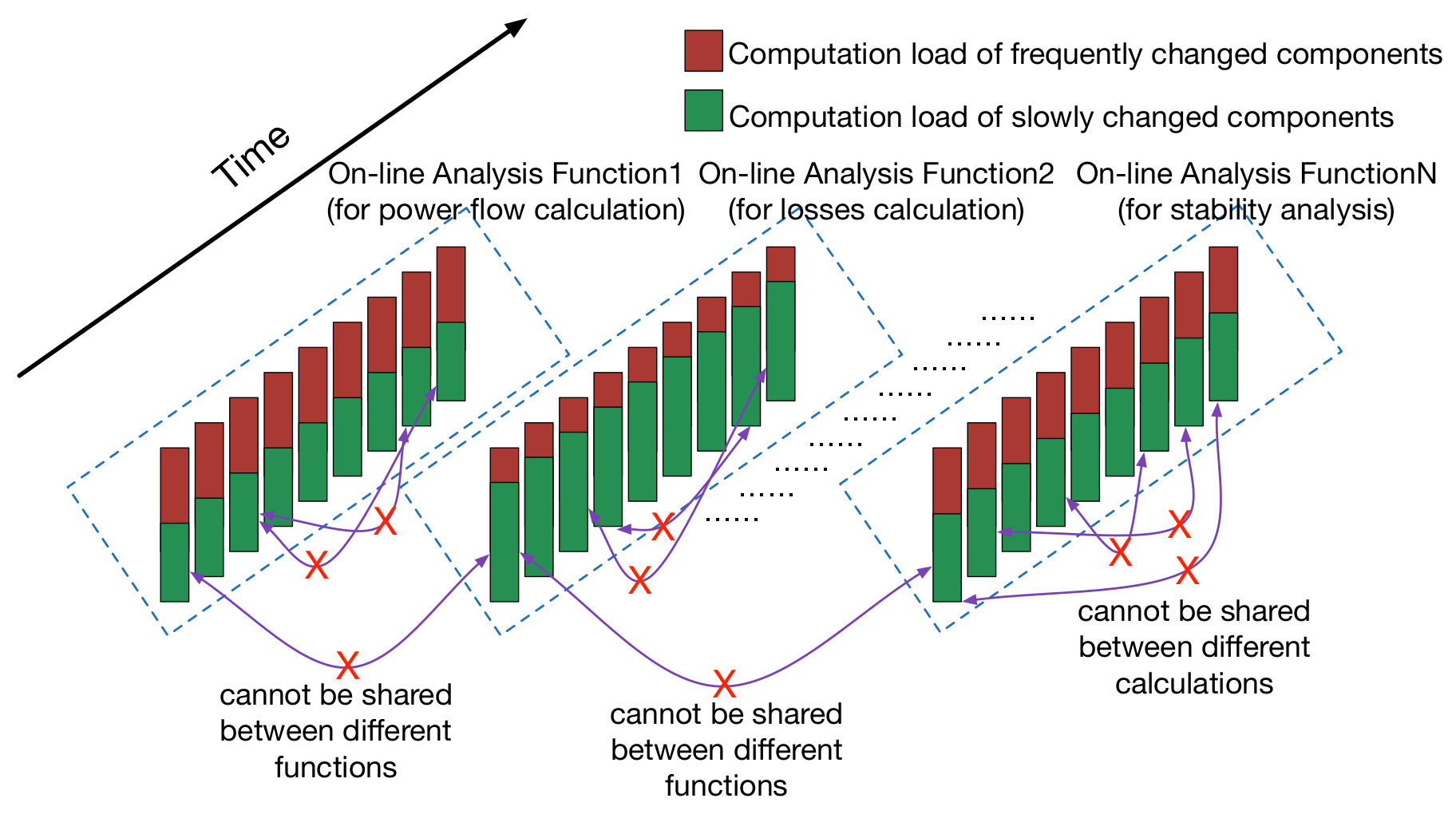
The analysis center of modern power system has many different functions to solve different problems. Typical functions include power flow calculation, steady state stability analysis, state estimation, optimization power flow, etc. Many functions need online operation and have to be performed again and again with time variation. The schematic diagram of the computation load of power system analysis center is shown in Figure 1. Each rectangle (which consists of red parts and green parts whose meanings will be explained in the following sections) represents the computation load of one-time computation of a function. The area of the rectangle stands for the computation load. Many functions may need to be performed simultaneously. Each function may need to be repeated frequently. The traditional research focuses on the improvement of one-time calculation of a problem, namely a single rectangle in Figure 1 (reducing the area of a single rectangle). This paper will focus on the improvement of holistic performance of the power system analysis center (reducing the total area of all rectangles).
2.2. The Repeated Analysis Computation Load
The formulas of many power system analysis problems are deeply coupled with the power grid. It can be briefly explained as follows:
- The derivation of the formulas is based on the power grid characters (such as topology, line parameters and bus types);
- Many power grid parameters are listed as constant coefficients of the formulas;
- The influence of each parameter variation on analysis results has to be calculated by solving nonlinear equations.
As a result, we can conclude that the power grid analysis is an important and implicit part of many power system analysis problems. However, we cannot obviously separate it from the calculation procedure as their relationships are mixed in the nonlinear formulas and the calculation procedure is performed by independent numerical iterative methods. Thus, the same power grid analysis has to be repeated among different calculations.
2.3. The Potentiality of the Holistic Performance
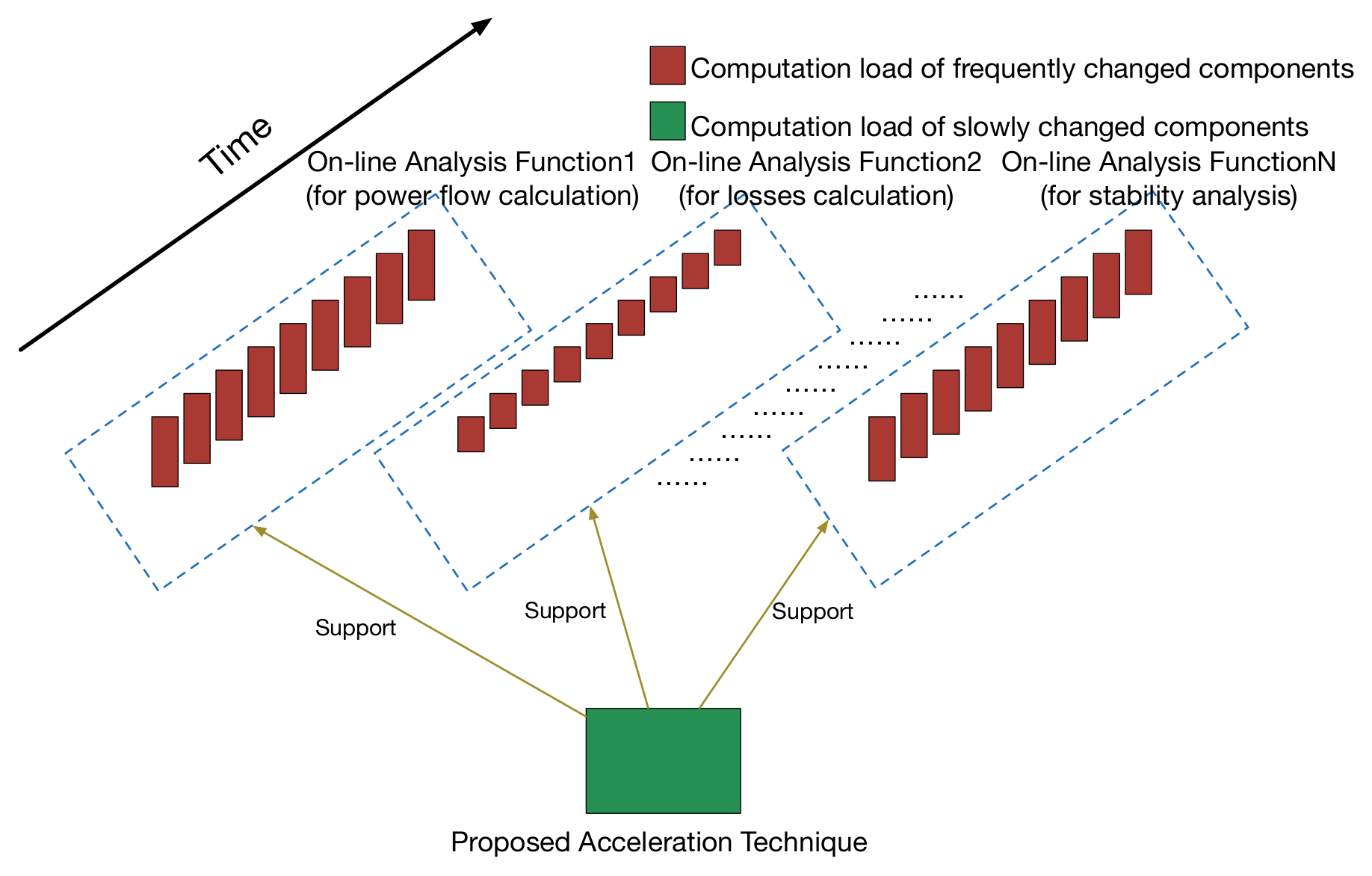
As the power grid parameters are relatively stable to the online analysis frequency, the same power grid analysis has to be repeated in each time calculation. If the power grid analysis can be (even partly) separated and directly used by each time calculation, the holistic performance of power system analysis can be much improved. The independent analysis of the power grid may need to pay much more time than any one-time single problem calculation; however, the holistic performance will be much improved with the increasing number of calculation time of different problems. In this paper, a technique will be proposed to separate the analysis of power grid whose results can be used by the calculation of different problems. The analysis results of the proposed technique can help to accelerate the speed of each time calculation of some problems. The schematic diagram of the analysis center computation load with independent power grid analysis is shown in Figure 2. The repeated computation of power grid analysis is avoided, but the proposed technique needs to pay some basic computation time. Thus, the proposed technique will show more advantages with the increase in function amount and calculation time. In addition, the separated power grid analysis results also reveal more relationships between different variables, which contributes to the system-level analysis of the complicated power system with many coupling subsystems and equipment. It will be analyzed in detail in the following sections.
3. The Linear Relationship Based Nonlinear Problem
In this section, the linear relationship based nonlinear problem (LRBNP) will be discussed in detail, which is the foundation of the proposed technique.
3.1. The Nonlinearity and Linearity of Power Systems
The power system is a typical complicated nonlinear system. The nonlinearity of the power system may come from the following aspects:
- The nonlinear equipment and components in power grids such as power electronic devices which are on the inside of power grids;
- The nonlinear characters of complicated loads and sources which are on the outside of power grids;
- The nonlinear mathematical relationships, for example, the relationship between powers and voltages.
The nonlinearity of (1) and (2) come from nonlinear elements itself. The nonlinearity of (3) comes from the product operation of linear variables. The power systems are strongly nonlinear systems. As a result, most power system problems have to be depicted as a set of nonlinear equations.
However, there are also many linear relationships and models in power system analysis. The models of lines and buses in power grids are linear in most power system problems. Thus, the circuit of the power grid is linear. As a result, the relationship between injected currents and bus voltages is linear, which is the basis of the derivation of power flow equations. In addition, small-signal models of nonlinear elements are also locally linear.
3.2. The Nonlinearity and Linearity in Power System Equations
The injected power equations are basic and typical nonlinear power system equations. The derivation procedure includes the following two main steps (both in AC and DC systems):
3.2.1. Establish the Relationship between Currents and Voltages
3.2.2. Get the Injected Powers Expression
Thus, we can conclude that the widely used injected power equations include linear elements, linear relationships and nonlinear relationships. No nonlinear elements are included.
In fact, we rarely use the nonlinear elements models in the calculation of power system analysis. Even the nonlinear power electronic devices are analyzed with small-signal models that are locally linearized models.
3.3. The Definition of Linear Relationship Based Nonlinear Problem
For analysis convenience, we define the problem like the injected power equations in Section 3.2 as linear relationship based nonlinear problem (LRBNP). The LRBNP only involves linear relationships, linear elements and nonlinear relationships, but no nonlinear element is involved. The nonlinear relationships only come from the product operation. In a power system problem involving nonlinear elements, if the nonlinear elements can be decoupled, the part without nonlinear elements can also be seen as LRBNP. Most classical power system analysis problems are LRBNPs.
The linear power grid models and relationships are used in almost all research of different problems. However, most nonlinear problems (include the basic power flow equations in textbook) ignore that their derivation implies the acknowledgement of the linear properties of power grid, although the forms of their equations are nonlinear. Thus, the nonlinear equations are solved directly with mathematical tools and the calculation procedures are seen as blackboxes. The ignorance makes the research not focus on the inside study of the problems, which results in the repeated redundant computation load in power system analysis center.
4. Explanation of Basic Principles of the Proposed Technique
4.1. The Frequently Changed and Slowly Changed Computation Load
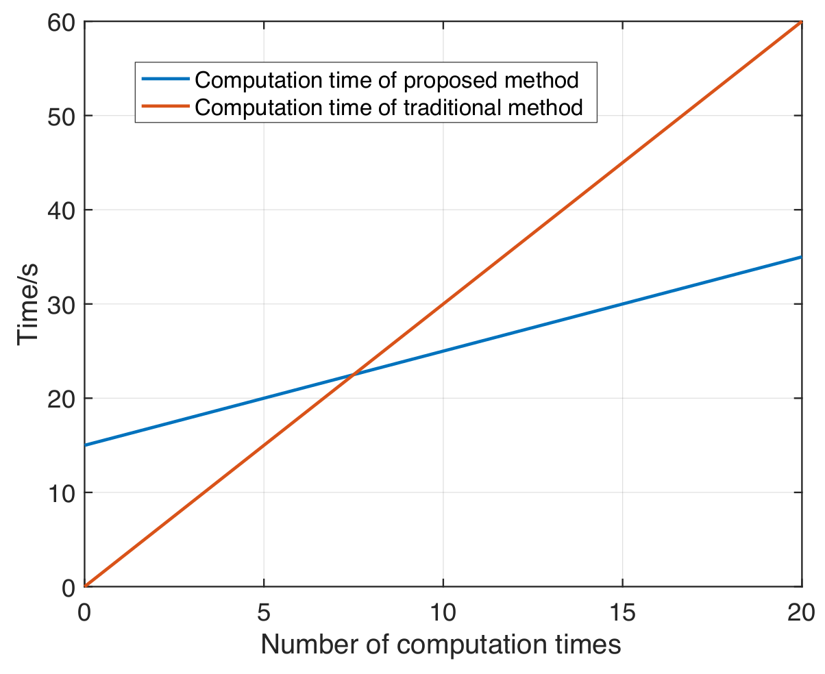
In many-time calculations of different power system analysis functions, some power grid parameters (such as line parameters, topology, bus parameters) are slowly changed, while the loads, sources and some other parameters are frequently changed. Combined with the complicated relationships in a specific problem, some computation load deals with the slowly changed parameters and some with the frequently changed parameters. If we only focus on a one-time calculation of a specific problem, the frequently changed and slowly changed computation load have no difference because they both only need to be calculated for only one time. In a practical power system analysis center, many different functions need to be performed for many times for the normal operation of the power system. It is hard to tell the frequently changed and slowly changed computation load in the calculation procedure, but we can conclude that the calculations repeat many-time same power grid analysis independently. In Figure 1 and Figure 2, the green color stands for the slowly changed computation load and the red color stands for the frequently changed computation load. The purpose of the two figures is to help to understand, and the areas of green and red colors are not strictly accurate. By avoiding the repeated computation load of slowly changed components, the holistic speed can be much improved. It can be seen that the total area of green color in Figure 2 is much smaller than Figure 1 if the calculation time is long enough. However, the green color area in Figure 2 is also larger than the green color area in any one-time calculation of a specific function. The green color in Figure 2 is the basic computation load of the proposed technique. However, it is obvious that the practical total computation load in a power system analysis center will be dramatically reduced by a proposed technique. The speed comparison of the traditional method and the method with the proposed technique is shown in Figure 3 (not strictly accurate but reflect the characters).
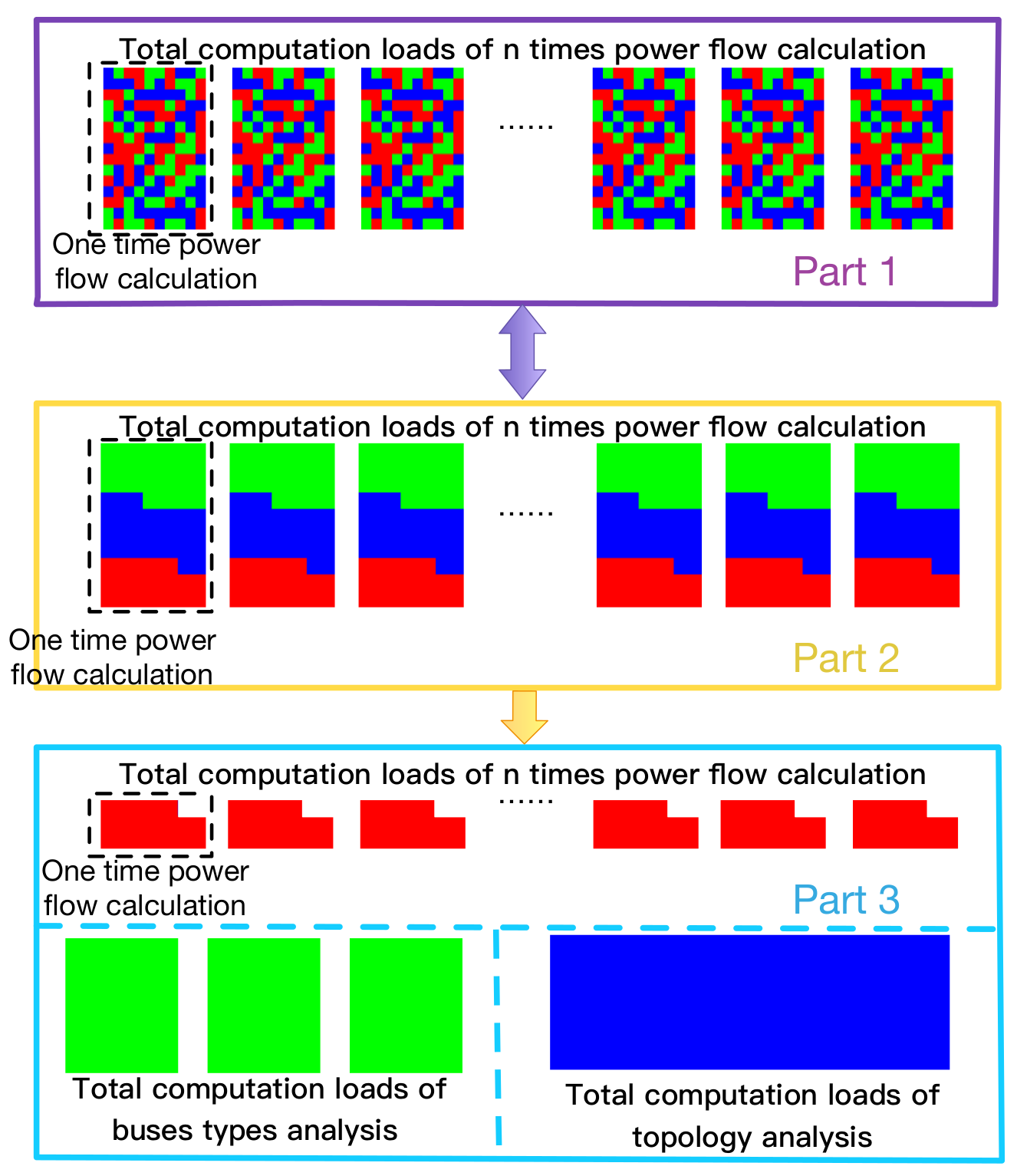
4.2. What the Proposed Technique Does
The proposed technique is based on the deep mathematical analysis of LRBNPs. It successfully separates the slowly changed computation load (power grid analysis) from the nonlinear equations. Thus, some analysis of power grids can be performed independently decoupling with specific nonlinear problems. The repeated slowly changed computation load just needs to be performed one time among different problem calculations. The power flow analysis is used as an example to show the meanings of the proposed technique. The components of power flow analysis computation load are shown in Figure 4. The red color represents the computation load of sources/loads information analysis. The green color represents the computation load of bus types analysis. The blue color represents the computation load of topology analysis (the blue and green color loads in Figure 4 correspond to the green slowly changed computation load in Figure 1 and Figure 2). As they have different variation frequencies, they are presented with different colors for better explanation in following sections). In traditional iterative methods, the three components are mixed together as shown in part 1 of Figure 4, and they cannot be separated. All of them have to be recalculated if any of them changes. Part 2 of Figure 4 is another equivalent representation form of part 1 for concise representation. The traditional iterative methods cannot separate the mixed computation load of part 1 like part 2. The proposed technique aims to provide a way to achieve the separation. If the computation load is separated successfully, the computation load can be equivalent to part 3 of Figure 4. Although the separation analysis of topology and bus types will spend extra time, it only needs to be performed for one time. After separation, only the sources/loads computation is needed in each power flow calculation. Thus, if the number of computation times is relatively small, the proposed method may be slower than traditional methods. However, the advantages of the proposed technique will be shown with an increasing number of computation times. For most power system analysis tasks, it can bring much benefits. Without loss of generality, the sources/loads computation in power flow analysis may be replaced by other specific problems, but the topology and bus types analysis are similar.
With the large number of total times, the improvement of holistic performance is possible, although the proposed technique needs to spend some time to complete the basic analysis. In addition, the proposed technique can deeply analyze the linear relationships of the power grid in detail. The new relationships also provide a new way to strictly understand the mathematical and physical meanings of power system problems. The new relationships reveal some new properties of power grids. It contributes to the system-level analysis of power systems. The detailed derivation and analysis will be presented in the following sections of this paper. Combined with the specific power system problems, new methods to solve the classical problems can be further proposed.
4.3. Separate the Computation Load with Different Variation Frequencies
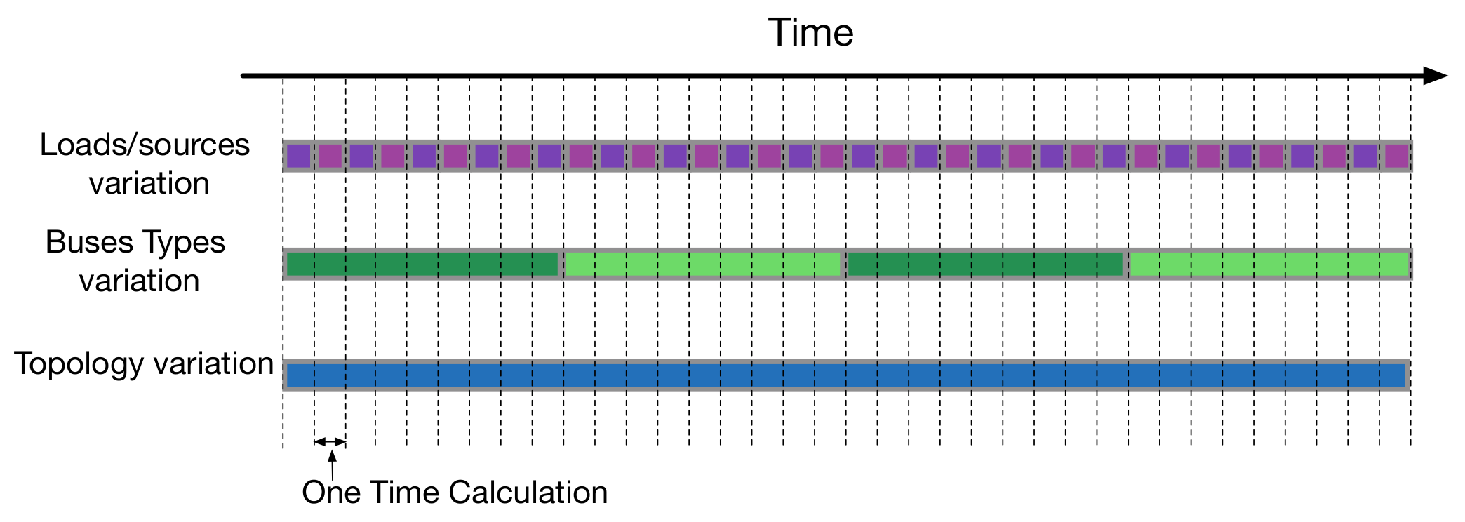
For a specific problem, it may involve many parameters such as topology, lines, bus types, loads/sources powers. In a practical system, these parameters have different variation frequencies. The loads/sources powers vary most frequently. The bus types may change with the operation modes of sources or loads, but their variation frequency is relatively slower. The topology and line parameters of a power system are stable for a very long time (months or years), and their variation frequency is the slowest. The proposed technique can separate the three types of analysis computation. Thus, the same repeated computation load can be minimized.
The total computation load of traditional many-time calculations of a problem is shown in Figure 5. Each line stands for one kind of computation load. If one kind of parameters changes, the color will also change, namely the change of the color in the same line means the variation of the parameters. As mentioned, the loads/sources vary the fastest and the topology varies the slowest, which can be seen in Figure 5. In Figure 5, the computation load of one-time calculation is between the same two adjacent dash lines.
With the analysis results of the proposed technique, the computation load of many-time calculations of a problem is like Figure 6. It can be seen that, if no variation occurs, the corresponding kind of parameters need not to be analyzed. Thus, some calculations only need to afford computation load of loads/sources and bus types. Some calculations only need to afford the computation load of loads/sources.
4.4. How to Solve the Nonlinear Equations
For most research, when the equations are obtained, some mathematical tools to solve nonlinear equations are directly used to get the solution. In this way, the derivation procedure and calculation procedure are separated. The analysis structure of traditional methods is shown in Figure 7. Combined with the power system problems to be solved, the nonlinear relationships, nonlinear elements, linear relationships, linear elements need to be organized and derived to form the nonlinear equations. Then, those are mixed together like a blackbox, and the mathematical tools are used to solve the nonlinear problems. In this structure, it is impossible to separate the slowly changed computation load and frequently changed computation load. The total computation time of the power system analysis center is the sum of many-time different problem calculations. The repeated same power grid analysis cannot be avoided.
The analysis structure of power system problems with the proposed technique is shown in Figure 8. This technique separates the linear relationships and linear elements of the power grid analysis from nonlinear equations. The linear part is analyzed with linear analysis methods. Compared with the linear properties used in traditional derivation, this technique analyzes much more deeply and the results can accelerate each one-time calculation. In addition, more relationships are revealed, which can help to analyze the deep coupling subsystems. Other nonlinear relationships and elements are combined with specific problems. However, the nonlinear partial analysis and linear partial analysis cannot be simply added to get the solutions. Thus, a new iterative method is very important to make the nonlinear part cooperate with the linear part to get accurate solutions. The new iterative method may be different in different problems.
4.5. Why the Proposed Technique Contributes to Deep Coupling Systems Analysis
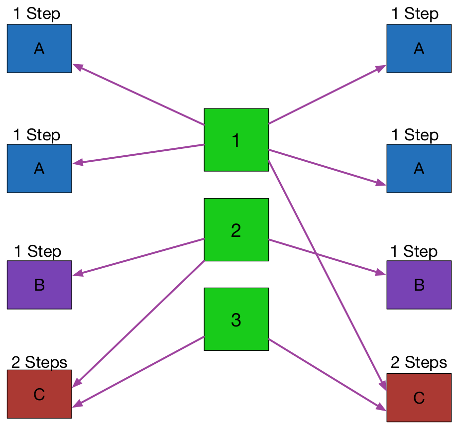
The modern power systems are deep-coupling systems that include the interaction among different devices (such as power electronics equipment, electrical vehicles, distributed generators and so on) and systems (such as communication systems, control systems and so on). In traditional methods, the linear properties of the power grid that are used to derive the nonlinear equations are relatively simple. As the linear properties are not deeply analyzed, some LRBNPs become more complicated than they should be. Because the analysis of the interaction needs the calculations of some nonlinear equations, the deep analysis of the linear properties can simplify the deep-coupling problems. The schematic diagram of the traditional relationship between the linear properties and power system problems is shown in Figure 9. The green boxes in the figure stand for the linear properties of the power grid. In the traditional method, only the linear relationship between injected currents and bus voltages in (1) is used, which is denoted as box 1 in the figure. Box 2 and box 3 stand for some other linear relationships in the power grid. The other linear relationships may be between injected currents and line currents, bus voltages and line currents, injected currents and line voltages, bus voltages and line voltages (the strict demonstration of the linearity will be presented in the next section). The blue boxes stand for the problems that can be directly derived with the linear relationship in (1). The purple boxes stand for the problems that need the information of line currents and line voltages. As the strict linear relationships between line currents (voltages) and injected currents (bus voltages) are not used, the information has to be obtained through the calculation of nonlinear equations. The system losses calculation is one kind of these problems. In traditional methods, the power flow calculation must be performed before the losses calculation to get the line currents. Then, the losses calculation can continue. It can be seen in Figure 9 that the losses calculation needs three steps. The first step is to solve another nonlinear problem (power flow calculation). The second step is to get the results (line currents) that have linear properties in the power grid. The third step is to calculate the system losses with the results in step 2. The red boxes stand for the power system problems involving multiple systems and devices coupling. Based on traditional methods, these kinds of problems will be much more complicated and need more steps between the nonlinear problems and linear properties.
With the deep analysis of linear properties derived by the proposed technique, Figure 9 can be improved to Figure 10. Some formulas can be derived directly from more specific linear relationships instead of the basic (1). With the simplification, the complicated coupling relationships are easier to handle.
5. Demonstration of the Linear Property
Although the steady state equations of power system are nonlinear, the nonlinearity does not come from the models of power grid. It comes from the nonlinear relationship between injected powers and bus voltages (or injected currents). Whether in DC or AC power systems, the linear models of lines and buses are used, and it is also an implicit condition of the Newton–Raphson method. In this section, the linearity of network is strictly analyzed. The following derivation of the proposed technique is based on the analysis of this section. Thus, although the demonstration only uses basic electric circuit knowledge, it is necessary to construct a strong and reliable theory foundation.
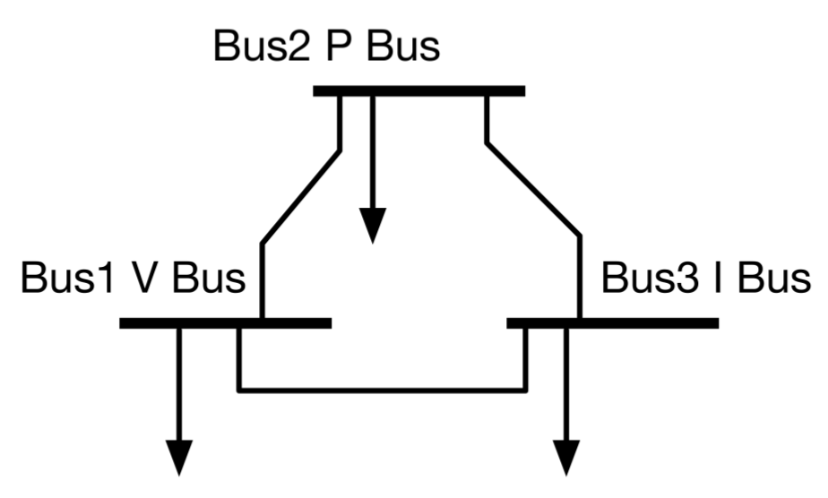
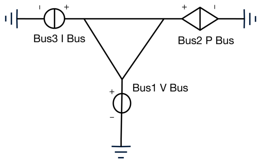
Without loss of generality, a simple power system with typical DC bus types (V bus, I bus and P bus) is used. The topology and the bus types are shown in Figure 11.
In view of electric circuit theory, the power system in Figure 11 is not a complete circuit. To make the circuit complete, some components should be added. If one bus has sources, an equivalent source should be added (voltage source at V bus and current source at I bus) between the injected point and ground (or neutral point in some system). If the bus is a load bus, a variable resistance should be added between injected point and ground (or neutral point in some systems). According to the replace theorem, the bus branch can be replaced by a current source (if the bus type is I bus) or a controlled current source (if the bus type is P bus). In this section, it is assumed that the V bus and I bus are all buses with sources. The complete circuit corresponding to the system in Figure 11 is shown in Figure 12. As a branch must exist between the injected point and the ground (or neutral point in some systems), the (controlled) voltage source and (controlled) current source can also be transformed equivalently according to the replace theorem.
Thus, the superposition theorem can be used to reveal the linear property, and the circuit in Figure 12 is equivalent to the circuit in Figure 13. It is obvious that currents in lines and the bus voltage drops have linear relationships with injected currents (or bus voltages).
The aforementioned analysis is based on the DC system. In the AC system, only the PV bus and PQ bus are considered and it is not difficult to get the same restrict conclusion.
6. Derivations of the Topology Separation
6.1. The Free Variables in the View of Electrical Circuit
Assume that the researched power system has N buses, and denote the injected currents vector as
All of the injected currents must satisfy
This means that the injected currents have N-1 degrees of freedom. Without loss of generality, assume the bus 1 is the reference bus in the DC power system. In the DC system, the bus type of the reference bus should be V bus to afford the power balance task. The voltage of V bus is specified and the injected current at bus 1 should be calculated by Equation (4) instead of a free variable. Based on the linear property of power grid demonstrated in Section 5, it can be inferred that the currents in lines and the voltage drops of all lines can be exactly determined by following free injected currents
In power system analysis, not any bus can be modeled as I bus, but I bus analysis can help the overall theory derivations. Following analysis in this paper will solve this problem after the relationships which are based on free injected currents are completely derived.
6.2. The Relationship between Injected Currents and Line Currents
Assume a power system has M lines, and the currents of lines are denoted as
According to the linear properties demonstrated in Section 5, the currents of lines can be linearly determined by the free injected currents through linear operation and the form is
where the A is a constant matrix determined by topology and power grid parameters,
Expand Equation (7), we get
6.3. The Method to Calculate the Matrix A
The matrix A includes the topology information about the linear relationship between injected currents and line currents. It has elements, and the elements are all constants if the topology and parameters are not changed. The aforementioned analysis only proves that the constant matrix A exist. However, how to calculate the matrix A is a problem.
According to Equation (9), each line current involves a row of matrix which has unknown elements. To solve the unknown elements, equations are needed. In each equation, the known variables should be one line current and injected currents which are the results of one-time power flow calculation. To get the equations, times traditional power flow calculations of the power system in different scenarios are needed. Denote the line currents of kth time power flow calculation as
Denote the injected currents of kth time power flow calculation as
Define the vector as
Define the vector as
Define the matrix H as
The relationship among , and H is
Each set of equations in Equation (15) comes from the results of N-1 times power flow calculations. The line currents and injected currents are all known variables calculated by power flow calculations in Equation (15) and the elements of matrix A are seen as unknown variables. The ith row of matrix A can be calculated by
For different i, the is same. With the , the A can be obtained:
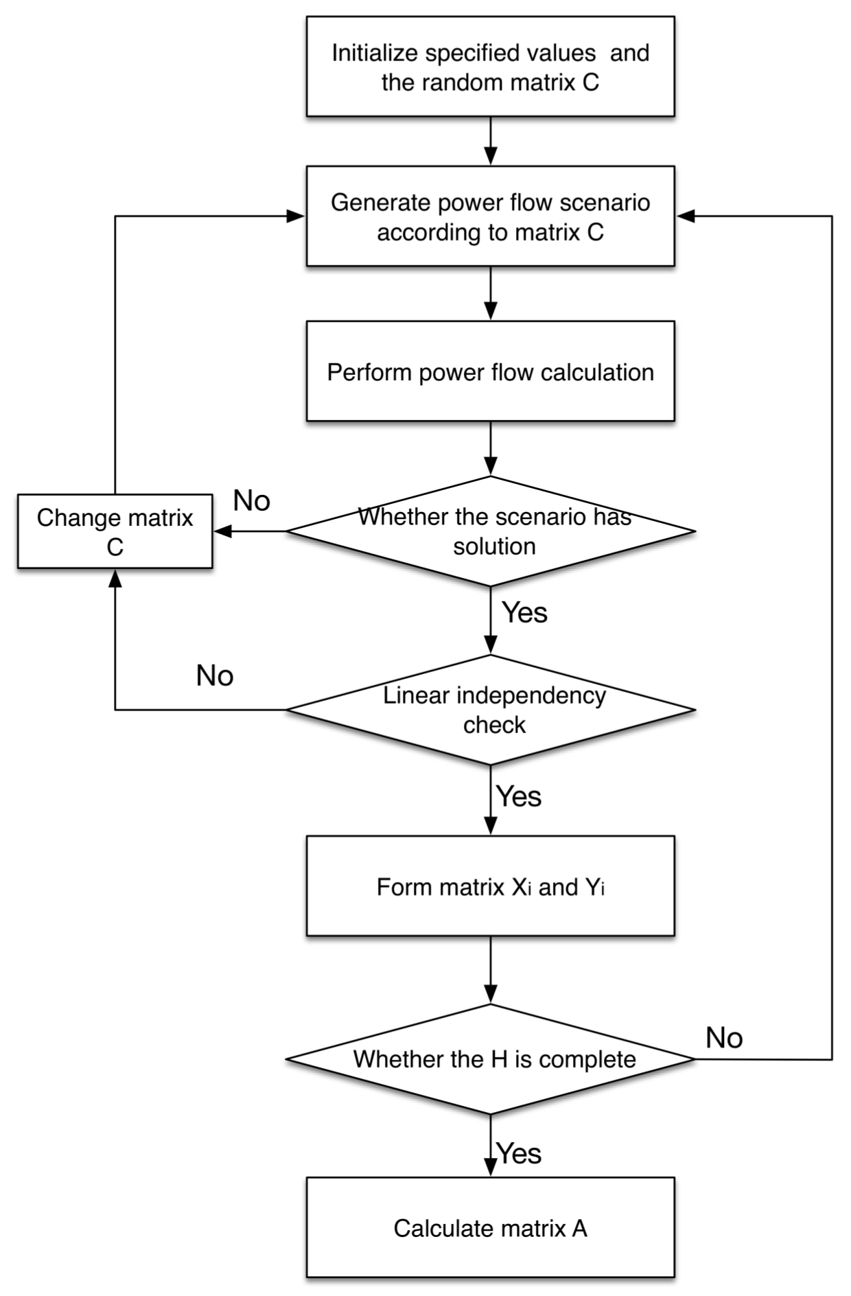
It is obvious that if the H is a singular matrix, the calculation of A will fail. The necessary and sufficient condition for the matrix H is not singular is that the all are linearly independent. To assure the non-singularity of H, each power flow calculation scenario cannot be arbitrary. With the following method, the singular matrix can be avoided.
Define a random matrix C:
All elements in the matrix C are independent variables and they all subject to uniform distribution:
The specified values of different types of buses should be changed according to matrix C in each time power flow calculation. If the bus i is a P bus or I bus, the specified value of bus i in kth time power flow calculation is set to () times:
If the bus i is a V bus, the specified value of bus i in kth time power flow calculation is set to () times:
, and are the basic specified values of corresponding buses.
It should be pointed out that the element of matrix C can subject to any distribution, as long as the variance is proper. If the variance is too small, the ill condition of matrix H may be caused. However, if the variance is too large, it may make power flow equations unsolvable. When calculating the matrix A, these situations should be considered.
The workflow of the calculation of the matrix A is shown in Figure 14. During the calculation, if one power flow scenario has no solution, or the calculation results destroy the linear independence of row vectors of the matrix H, the results should be discarded. The new corresponding row of matrix C should be regenerated and power flow calculation should be performed again.
6.4. The Relationship between Injected Currents and Bus Voltage Drops
Based on the linear properties, the relationship between bus voltage drops and injected currents can be further calculated. The voltage drops of each line can also be directly calculated with the line currents and line resistances (impedances in AC system). If the voltage of the reference bus is given, the voltage of every bus can be calculated by injected currents through linear calculation. To calculate the total bus voltage drops, the paths from the reference bus to other buses should be selected. The total voltage drops of a bus are equal to the sum of all line voltage drops in the path. To decrease the computation load, the shortest path is the best selection to calculate the total voltage drops. The Dijkstra algorithm is a well-known algorithm for the shortest path calculation in graph theory. It is used here to get the shortest path in a complicated meshed power system. It only needs to be performed for one time if the topology is not changed.
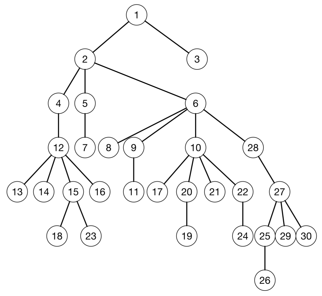
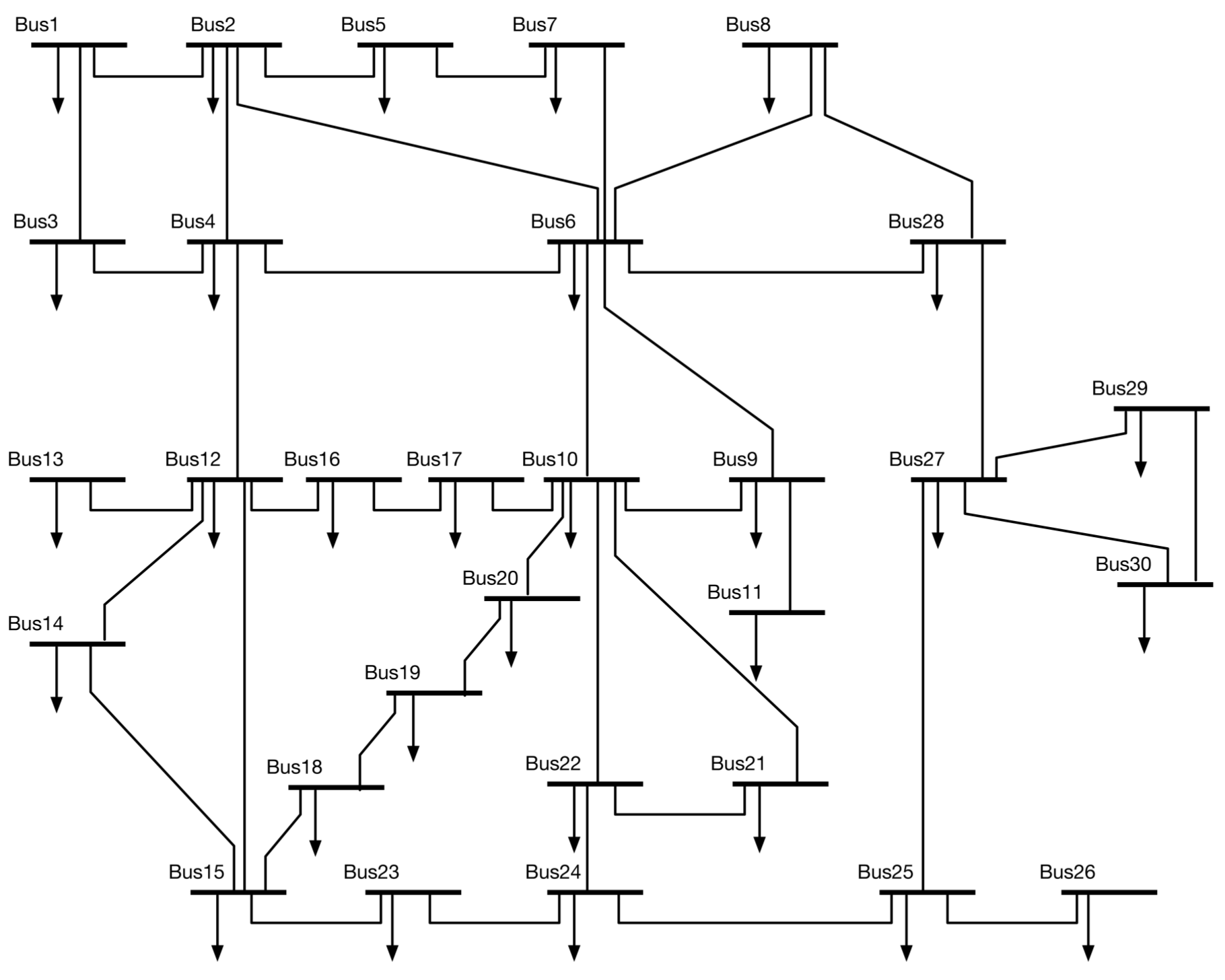
The IEEE 30 bus system is shown in Figure 15. With the Dijkstra algorithm, the shortest paths of all buses can be obtained and the meshed topology can be converted to a tree as shown in Figure 16.
For the buses, sets are used to represent the shortest paths:
If the jth line is in the shortest path from the reference bus to bus i, it means
The voltage of jth bus can be expressed as
To simplify the expressions, the matrix is defined as
The element of the matrix can be expressed as
Define the vector as
The expressions of Equation (25) can be equivalent to
With the above derivations, the line currents and bus voltage drops are successfully linearly expressed by the injected currents, which is coincident with the linearity demonstrated in Section 5. The coefficients are all constants.
6.5. The Separation of Topology Analysis
Actually, matrix A and matrix contain the information of power topology that is not taken full advantage of in traditional derivations. Matrix A and matrix are totally determined by the power grid. If the power grid structure is not changed, its matrix A and matrix will not be changed. Their analysis is independent with specific power flow problems. If some power system problems are based on the two matrices, the topology analysis does not need to be repeated in each time calculation, which cannot be avoided in traditional methods. Thus, the topology analysis is successfully separated.
7. The Derivation of Bus Types Separation
7.1. The Analysis of V Buses
If the bus k is a V buses, the voltage difference between the reference bus 1 and bus k is a constant. If there are V buses (not include the reference bus), define the V bus voltage drops vector as
where the Vi is the bus number of the ith V buses (). According to (25), the vector can also be expressed by the injected currents vector as
where is × () submatrix of constant matrix . It is easy to know that all the lines’ corresponding V buses in matrix consist of the matrix .
Assume there are P buses and I buses. To simplify the following analysis, define the injected currents vector of V buses as
Define the injected currents vector of P buses as
where the is the bus number of the ith P bus ().
Define the injected currents vector of I buses as
where the Ii is the bus number of the ith I bus ().
In Section 2, the number of independent injected currents is reduced to by the injected currents’ balance condition (4). Equation (31) establishes the relationship between the V bus voltage drops vector and the injected currents vector . If Equation (31) is seen as a set of constraint conditions, and the number of independent injected currents can be reduced to . It means that only the injected currents of P buses and I buses consist of the independent variables. From the view of a linear circuit, the influence of V buses on line currents and line voltage drops are linear.
7.2. The Discussion of P Buses
Obviously, the injected currents of P buses are in fact not independent variables like I buses because the relationship between power and current is nonlinear. The effects of P buses cannot be directly calculated by the results of this paper like V buses and I buses. However, it will not affect the strict derivations of this paper, and this problem will be overcome by the proper correction method. As the technique in this paper is complete and the paper length is limited, the relative content will be given in the future.
7.3. The Separation of V Buses
Denote the independent currents vector as
Sort according to bus types and we get
Rearrange the elements of to get the . The should satisfy
Let the consist of the 1 to columns of and the consist of the to columns of . The is a matrix and is a matrix. Equation (31) can be converted to another equivalent form
Isolating , we get
It means that, if the voltages of all V buses are given, the injected currents at V buses (except the reference bus) can be expressed by the injected currents of P buses and I buses. Thus, the system only has independent variables.
To separate bus types from power system analysis, a transformation matrix T and a constant vector are used to construct the relationship between and . They make the following equation correct:
The transformation matrix T is a matrix. If the bus i is a P bus or I bus and the injected current of bus i corresponds to the jth elements of , all the elements at ith row of T are 0 except the jth element at ith row is 1. If the bus i is a V bus, the ith row of T is the same as the row of which corresponds to the same V bus.
If the bus i is a P bus or I bus, the th element of is set to 0, if the bus i is a V bus, the th element of is the same as the element of which corresponds to the same V bus.
To get a clearer result, use the instead of . The transformation matrix T should be rearranged to and the should be rearranged to . The and satisfy
The can be expressed as
where the E is the identity matrix.
The can be expressed as
Denote the specified bus voltages vector of V buses as
Another transformation matrix can be used to express the as
where is an () × matrix. The is the specified voltage value of the reference bus. The subtraction between the scalar and the vector is the same as the subtraction in MATLAB (R2016b, Mathworks, Natick, MA, USA), namely the scalar is thought to be a vector whose size is the same as but every element is . The result is still .
Substituting Equation (47) with Equation (46), we get
7.4. The Separation of I Buses and P Buses
Divide the matrix AT, matrix and vector respectively, we get
and are all submatrices of T. The consists of the P columns of T and the consists of the I columns of T:
Denote
We get
Denote
We get
7.5. The Separation of Bus Types Analysis
All the matrices , , , , and are constant matrices, if the topology and bus types are not changed. If the topology is changed, all of them should be recalculated. If the topology is not changed, but the bus types are changed, the matrix A and can still be used, but the other vectors and matrices should be recalculated. The six constant matrices are the results of separation analysis of bus types, which are the foundation for further analysis. They can also reveal some new analytical relationships that are difficult to be obtained in traditional methods.
The bus types’ characters have been successfully separated. According to (52) and (50), the line currents and bus voltage drops of a power system are divided into the reference bus voltage term, V buses term, I buses term and P buses term. Except for the injected currents of P buses, all other values are known variables. In addition, all the coefficient matrices are constant and the operations are linear. If the exact injected powers have to be satisfied, it can be achieved with the other correction technique.
8. Discussion
8.1. The New Way to Understand a Power System
In traditional analysis of power system, it is difficult to tell where the power produced by a generator go or where the power of loads comes from. The above results could explain it. How much current in a line comes from each bus can be exactly expressed by the matrix A. As the variation of bus voltage in the DC system is relatively small, the current relationships can be converted to power relationships without much loss of accuracy. In the matrix A, the element means that the times injected power of bus j flows into transmission line i. Thus, the injected power routine of every bus can be calculated. The power margin of each line in a specific direction can also be approximately analyzed. Due to the limitation of length, these problems will not be deeply analyzed.
8.2. The Discussion of Application on AC Power Systems
It has been simply pointed out that the basic ideas and principles of proposed technique are applicable to both AC and DC power systems, although the research of this paper is mainly based on DC power systems. The linear relationships in DC power systems can also be exactly analogous to AC systems because the linear properties of networks are the same except that some complex coefficients may be involved. The complex coefficients have no influence on the linear properties. However, compared with DC systems, the application in AC systems still has some disadvantages.
The proposed technique in AC power systems may be less accurate than DC systems (although the accuracy is enough and can be further improved by more detailed derivation). The loss of accuracy comes from the model of the AC line, which has line-to-ground capacitance and equivalent conductance. In the model, the currents at two ends are different, which conflicts with the basic ideas of the proposed technique and destroys the exact linear relationship between injected currents and line currents. However, as the influence of line-to-ground capacitance and equivalent conductance is small, the technique can also be trusted.
As the capacity of the DC power system is much larger than the AC, the voltage changes of the DC system are much smaller than the AC system when the same power variation occurs. This advantage is also important for the proposed technique in DC power systems because the nonlinear variable power needs to be approximately converted to the current for analysis. The influences are (1) if the proposed technique is used for direct estimation, the accuracy will be higher in DC systems; (2) if the proposed technique is used for accurate calculation, the correction speed is faster in DC systems.
In a word, the proposed technique can be used either in DC and AC power systems, but better performance will be shown in DC power systems.
9. Verification of the Proposed Technique
9.1. Test Systems
To verify the proposed technique, typical test systems are required. However, to the best knowledge of the authors, no standard DC test systems can be found. The DC power system experiments are mainly performed in DC micro-grid and no practical DC distribution systems data can be easily found. To get the test scenarios, the standard IEEE 14 buses, IEEE 30 buses and IEEE 118 buses AC systems are modified. The modification observes the following rules:
- The topology of each network is not changed;
- The PV buses are converted to V buses and PQ buses are converted to P buses;
- The resistances of the lines in DC systems are specified according to the reactances of the lines in AC system;
- In the bipolar DC systems, the positive and negative phases are thought to be balanced;
- Some P buses and V buses may be replaced by I buses.
To assure the reasonability of the DC test systems, two validation methods are applied.
- Each test system is solved with the Newton–Raphson method to validate the reasonability. The results show that the converted test systems can exist.
- The topology, components and parameters of each test system are established and tested in SIMULINK. The simulation results prove that the modification is reasonable.
Due to the limitation of length, the data of the systems is presented in attachments. The file names of the three test systems are 14_buses_information.xlsx, 30_buses_information.xlsx and 118_buses_information.xlsx, respectively.
Each file has five parts. Part 1 gives the specified bus voltages. Part 2 is the specified bus and injected powers. Part 3 is a matrix, if the 1st column of ith row is set to 1, it means the bus i is a V bus; if the 2nd column of ith row is set to 1, it means the bus i is a P bus. Part 4 gives the information about lines. The first column of Part 4 gives the number from buses, the second column of Part 4 gives the number of buses, and the third column of Part 4 gives the resistances of lines. Part 5 is the conductance matrix of the DC power system.
9.2. 14 Buses Case
According to the derivation, the constant matrices A and are presented in Table 1 and Table 2, respectively. The constant matrices AT and T are presented in Table 3 and Table 4, respectively. The constant vectors A and are presented in Table 5.
To verify the accuracy of the proposed linear relationships, the traditional Newton–Raphson method is used in DC test systems to get the exact line currents and the bus voltage drops. Then, the line currents and the bus voltage drops will be calculated by Equations (7), (47), (29) and (48). With the injected currents calculated by Newton–Raphson method, the calculation results are listed in Table 6 and Table 7. The maximized error among the three methods is 4.3177 , which can be thought to be exact (most of the errors may come from the accumulation of truncation errors). Thus, it can be concluded that proposed linear relationships are exactly accurate.
9.3. 30 Buses Case
The verification in a 30 buses system is similar to the 14 buses system. Due to the limitation of length, the results are presented in attachment 30_buses_data.xlsx. The order and the forms of the results are similar to Section 9.2. The maximized error among the three methods in a 30 buses case is 1.5085 × 10.
9.4. 118 Buses Case
The verification in a 118 buses system is similar to the 30 buses system. The results are presented in attachment 118_buses_data.xlsx. The maximized error among the three methods in a 118 buses case is 3.1579 × 10. It can be seen that the maximized errors in 30 buses and 118 buses are larger than 14 buses system, although the absolute values are still extremely small. This is because the errors come from the accumulation of truncation errors and the larger system involves more accumulation. With the increase of the system scale, more errors will be accumulated in a one-time operation. However, the absolute value of the maximized error is so small that they can be completely neglected.
10. Conclusions
In this paper, a complete novel technique to improve the holistic performance of nonlinear power system problems are presented. The potentiality of the holistic performance of power system analysis center is pointed out. The ideas and principles of the technique are also explained in detail. The complete linear circuit properties of classical power system problems are strictly demonstrated. The mathematical formulas are derived in detail with strict demonstration. The topology analysis and bus types analysis are successfully separated. They are abstracted to constant matrices and the computation is simplified to linear operation. The results come from the deep research of the unused linear relationships of popular LRBNPs in power systems. This paper constructs the strong foundation for further specific nonlinear power system problems, which can improve the holistic performance of power system analysis center. The results also provide a new way to understand the power systems and it is emphasized that the derivations can be analogous to an AC system. The formulas are also proved to be accurate by numerical verification. Based on the works of this paper, the performance of some specific nonlinear power system problems can be dramatically improved.
Supplementary Materials
Supplementary File 1Author Contributions
Y.W. and Q.X. conceived and designed the experiments; Y.W. wrote the paper; Y.W. and M.C. analyzed the data; Y.W. and J.Z. contributed simulation tools.
Funding
This article is supported by the Science and Technology Project of SGCC under Grant (SGJSJX00YJJS1800721) and The National Key R&D Program of China under Grant (2017YFA0700300).
Conflicts of Interest
The authors declare no conflict of interest.
Abbreviations
| LRBNP | Linear relationship based nonlinear problem |
| AC | Alternative current |
| RES | Renewable energy resources |
| DC | Direct current |
| GGDF | Generalized generation shift distribution factor |
| GSDF | generation shift distribution factor |
| ZBD | Z-bus distribution factor |
| PTDF | Power transfer distribution factor |
| JBDF | Jacobian based distribution factor |
| PV | Constant power and voltage |
| PQ | Constant active power and reactive power |
References
- Saadat, H. Power System Analysis; WCB/McGraw-Hill: New York, NY, USA, 1999. [Google Scholar]
- Kamel, S.; Jurado, F. Fast decoupled load flow analysis with SSSC power injection model. IEEJ Trans. Electr. Electron. Eng. 2014, 9, 370–374. [Google Scholar] [CrossRef]
- Chen, T.H.; Chen, M.S.; Hwang, K.J.; Kotas, P.; Chebli, E.A. Distribution system power flow analysis-a rigid approach. IEEE Trans. Power Deliv. 1991, 6, 1146–1152. [Google Scholar] [CrossRef]
- Chen, H.Y.; Chen, J.F.; Duan, X.Z. Study on Power Flow Calculation of Distribution System with DGs. Autom. Electr. Power Syst. 2006, 1, 008. [Google Scholar]
- Glover, J.D.; Sarma, M.; Overbye, T. Power System Analysis & Design, SI Version; Cengage Learning: Boston, MA, USA, 2011. [Google Scholar]
- Kim, H.J.; Lee, Y.S.; Lee, J.G.; Han, B.M. Operation analysis of bipolar DC distribution system with voltage balancer. In Proceedings of the 2014 Australasian Universities Power Engineering Conference (AUPEC) 2014, Perth, WA, Australia, 28 September–1 October 2014; pp. 1–6. [Google Scholar]
- Gomes, F.V.; Carneiro, S.; Pereira, J.L.R.; Vinagre, M.P.; Garcia, P.A.N.; De Araujo, L.R. A new distribution system reconfiguration approach using optimum power flow and sensitivity analysis for loss reduction. IEEE Trans. Power Syst. 2006, 21, 1616–1623. [Google Scholar] [CrossRef]
- Chen, S.T.; Huang, W.T.; Lai, W.T.; Shi, P.H. Power System Fast Line Flow Calculation for Security Control by Sensitivity Factor. In Proceedings of the Second International Conference on Innovative Computing, Informatio and Control (ICICIC 2007), Kumamoto, Japan, 5–7 September 2007; p. 98. [Google Scholar]
- Wang, Y.; Xu, Q.; Liu, M.; Zheng, J. A novel system operation mode with flexible bus type selection method in DC power systems. Int. J. Electr. Power Energy Syst. 2018, 103, 1–11. [Google Scholar] [CrossRef]
- Balog, R.S.; Weaver, W.W.; Krein, P.T. The load as an energy asset in a distributed DC smartgrid architecture. IEEE Trans. Smart Grid 2012, 3, 253–260. [Google Scholar] [CrossRef]
- Dong, D.; Cvetkovic, I.; Boroyevich, D.; Zhang, W.; Wang, R.; Mattavelli, P. Grid-interface bidirectional converter for residential DC distribution systems—Part one: High-density two-stage topology. IEEE Trans. Power Electron. 2013, 28, 1655–1666. [Google Scholar] [CrossRef]
- Wang, Y.; Xu, Q.; Ma, Z.; Zhu, H. An Improved Control and Energy Management Strategy of Three-Level NPC Converter Based DC Distribution Network. Energies 2017, 10, 1635. [Google Scholar] [CrossRef]
- Saeedifard, M.; Graovac, M.; Dias, R.F.; Iravani, R. DC power systems: Challenges and opportunities. In Proceedings of the Power and Energy Society General Meeting, Providence, RI, USA, 25–29 July 2010; pp. 1–7. [Google Scholar]
- Choi, B. Pulsewidth Modulated DC-to-DC Power Conversion: Circuits, Dynamics, and Control Designs; John Wiley & Sons: Hoboken, NJ, USA, 2013. [Google Scholar]
- Radwan, A.A.A.; Mohamed, Y.A.R.I. Linear active stabilization of converter-dominated DC microgrids. IEEE Trans. Smart Grid 2012, 3, 203–216. [Google Scholar] [CrossRef]
- She, X.; Lukic, S.; Huang, A.Q. DC zonal micro-grid architecture and control. In Proceedings of the IECON 2010-36th Annual Conference on IEEE Industrial Electronics Society, Glendale, AZ, USA, 7–10 November 2010; pp. 2988–2993. [Google Scholar]
- Kakigano, H.; Miura, Y.; Ise, T. Configuration and control of a DC microgrid for residential houses. In Proceedings of the Transmission & Distribution Conference & Exposition: Asia and Pacific, Seoul, South Korea, 26–30 October 2009; pp. 1–4. [Google Scholar]
- Chen, D.; Xu, L. Autonomous DC voltage control of a DC microgrid with multiple slack terminals. IEEE Trans. Power Syst. 2012, 27, 1897–1905. [Google Scholar] [CrossRef]
- Radwan, A.A.A.; Mohamed, Y.A.R.I. Assessment and mitigation of interaction dynamics in hybrid ac/dc distribution generation systems. IEEE Trans. Smart Grid 2012, 3, 1382–1393. [Google Scholar] [CrossRef]
- Yao, J.; Li, H.; Liao, Y.; Chen, Z. An improved control strategy of limiting the DC-link voltage fluctuation for a doubly fed induction wind generator. IEEE Trans. Power Electron. 2008, 23, 1205–1213. [Google Scholar]
- Hagiwara, M.; Akagi, H. An approach to regulating the DC-link voltage of a voltage-source BTB system during power line faults. IEEE Trans. Ind. Appl. 2005, 41, 1263–1271. [Google Scholar] [CrossRef]
- Wang, C.; Li, X.; Guo, L.; Li, Y.W. A nonlinear-disturbance-observer-based DC-bus voltage control for a hybrid AC/DC microgrid. IEEE Trans. Power Electron. 2014, 29, 6162–6177. [Google Scholar] [CrossRef]
Figure 1.
Computation load of the power system analysis center.

Figure 2.
Computation load of the power system analysis center.

Figure 3.
Speed comparison.

Figure 4.
Schematic diagram of the proposed technique idea.

Figure 5.
Power system analysis without the proposed technique.

Figure 6.
Power system analysis without the proposed technique.
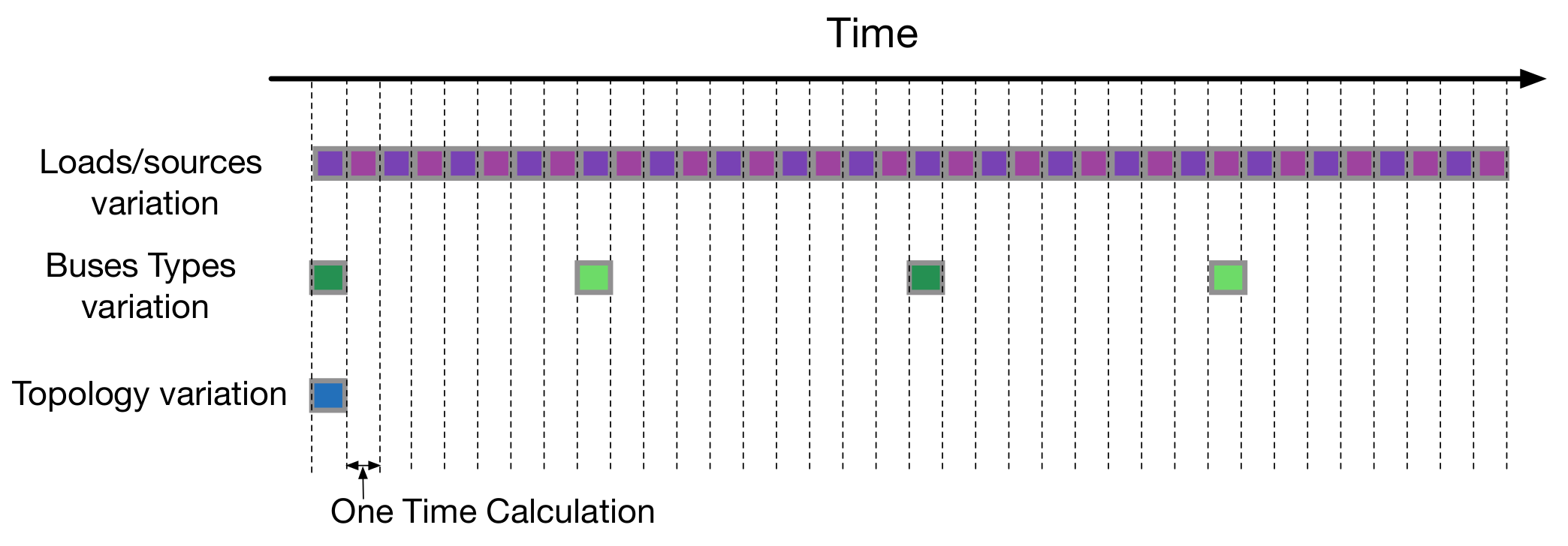
Figure 7.
Power system analysis without a proposed technique.
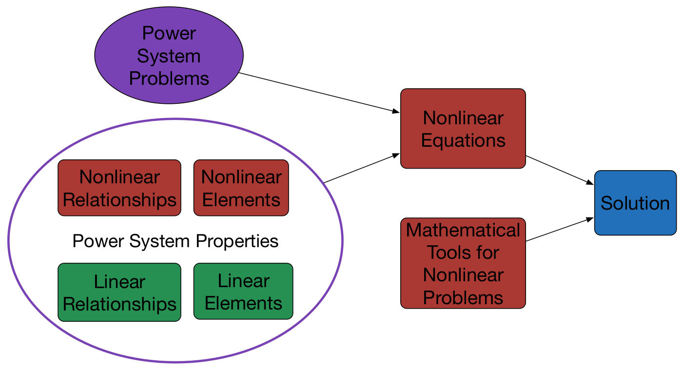
Figure 8.
Power system analysis with the proposed technique.
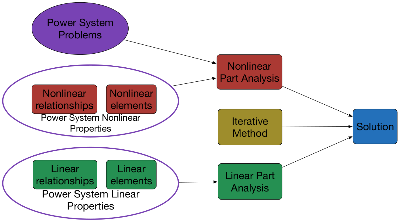
Figure 9.
Schematic diagram of the traditional relationship between the linear properties and power system problems.
Figure 9.
Schematic diagram of the traditional relationship between the linear properties and power system problems.

Figure 10.
Schematic diagram of the relationship between the linear properties and power system problems in the proposed technique.
Figure 10.
Schematic diagram of the relationship between the linear properties and power system problems in the proposed technique.

Figure 11.
A simple power system.

Figure 12.
Complete circuit of the simple power system.

Figure 13.
Superposition theorem for the simple power system.
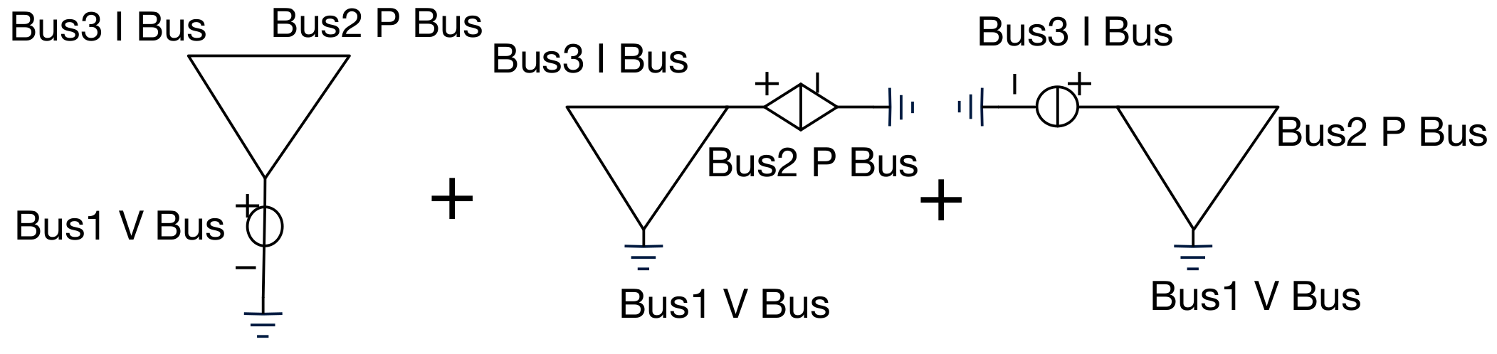
Figure 14.
Workflow of matrix A calculation.

Figure 15.
IEEE 30 bus system.

Figure 16.
Tree of IEEE 30 bus system.

Table 1.
Matrix A in a 14 buses system.
| 1 | 2 | 3 | 4 | 5 | 6 | 7 | 8 | 9 | 10 | 11 | 12 | 13 | |
|---|---|---|---|---|---|---|---|---|---|---|---|---|---|
| 1 | −0.8380 | −0.7465 | −0.6675 | −0.6106 | −0.6299 | −0.6573 | −0.6573 | −0.6519 | −0.6480 | −0.6391 | −0.6317 | −0.6330 | −0.6437 |
| 2 | −0.1620 | −0.2535 | −0.3325 | −0.3894 | −0.3701 | −0.3427 | −0.3427 | −0.3481 | −0.3520 | −0.3609 | −0.3683 | −0.3670 | −0.3563 |
| 3 | 0.0273 | −0.5320 | −0.1514 | −0.1031 | −0.1195 | −0.1427 | −0.1427 | −0.1382 | −0.1348 | −0.1273 | −0.1210 | −0.1221 | −0.1311 |
| 4 | 0.0572 | −0.1434 | −0.3168 | −0.2157 | −0.2501 | −0.2987 | −0.2987 | −0.2891 | −0.2822 | −0.2664 | −0.2532 | −0.2556 | −0.2745 |
| 5 | 0.0774 | −0.0711 | −0.1994 | −0.2918 | −0.2604 | −0.2159 | −0.2159 | −0.2246 | −0.2310 | −0.2454 | −0.2575 | −0.2553 | −0.2381 |
| 6 | 0.0273 | 0.4680 | −0.1514 | −0.1031 | −0.1195 | −0.1427 | −0.1427 | −0.1382 | −0.1348 | −0.1273 | −0.1210 | −0.1221 | −0.1311 |
| 7 | 0.0800 | 0.3071 | 0.5033 | −0.3016 | −0.0279 | 0.3589 | 0.3589 | 0.2830 | 0.2278 | 0.1021 | −0.0034 | 0.0158 | 0.1662 |
| 8 | 0.0029 | 0.0111 | 0.0182 | −0.0109 | −0.2171 | −0.6342 | −0.6342 | −0.4513 | −0.4097 | −0.3151 | −0.2356 | −0.2501 | −0.3633 |
| 9 | 0.0017 | 0.0064 | 0.0104 | −0.0062 | −0.1246 | −0.1661 | −0.1661 | −0.2590 | −0.2351 | −0.1808 | −0.1352 | −0.1435 | −0.2085 |
| 10 | −0.0045 | −0.0174 | −0.0286 | 0.0171 | −0.6584 | −0.1997 | −0.1997 | −0.2897 | −0.3552 | −0.5041 | −0.6292 | −0.6065 | −0.4282 |
| 11 | −0.0027 | −0.0105 | −0.0172 | 0.0103 | 0.2057 | −0.1202 | −0.1202 | −0.1744 | −0.2846 | −0.5350 | 0.1757 | 0.1522 | −0.0316 |
| 12 | −0.0004 | −0.0015 | −0.0025 | 0.0015 | 0.0302 | −0.0177 | −0.0177 | −0.0256 | −0.0157 | 0.0069 | −0.5201 | −0.1687 | −0.0882 |
| 13 | −0.0014 | −0.0054 | −0.0088 | 0.0053 | 0.1057 | −0.0618 | −0.0618 | −0.0896 | −0.0549 | 0.0240 | −0.2849 | −0.5900 | −0.3084 |
| 14 | 0.0000 | 0.0000 | 0.0000 | 0.0000 | 0.0000 | 0.0000 | −1.0000 | 0.0000 | 0.0000 | 0.0000 | 0.0000 | 0.0000 | 0.0000 |
| 15 | 0.0029 | 0.0111 | 0.0182 | −0.0109 | −0.2171 | 0.3658 | 0.3658 | −0.4513 | −0.4097 | −0.3151 | −0.2356 | −0.2501 | −0.3633 |
| 16 | 0.0027 | 0.0105 | 0.0172 | −0.0103 | −0.2057 | 0.1202 | 0.1202 | 0.1744 | −0.7154 | −0.4650 | −0.1757 | −0.1522 | 0.0316 |
| 17 | 0.0018 | 0.0069 | 0.0114 | −0.0068 | −0.1359 | 0.0794 | 0.0794 | 0.1152 | 0.0706 | −0.0308 | −0.1951 | −0.2413 | −0.6034 |
| 18 | 0.0027 | 0.0105 | 0.0172 | −0.0103 | −0.2057 | 0.1202 | 0.1202 | 0.1744 | 0.2846 | −0.4650 | −0.1757 | −0.1522 | 0.0316 |
| 19 | −0.0004 | −0.0015 | −0.0025 | 0.0015 | 0.0302 | −0.0177 | −0.0177 | −0.0256 | −0.0157 | 0.0069 | 0.4799 | −0.1687 | −0.0882 |
| 20 | −0.0018 | −0.0069 | −0.0114 | 0.0068 | 0.1359 | −0.0794 | −0.0794 | −0.1152 | −0.0706 | 0.0308 | 0.1951 | 0.2413 | −0.3966 |
Table 2.
Matrix in a 14 buses system.
| 1 | 2 | 3 | 4 | 5 | 6 | 7 | 8 | 9 | 10 | 11 | 12 | 13 | |
|---|---|---|---|---|---|---|---|---|---|---|---|---|---|
| 1 | −0.0496 | −0.0442 | −0.0395 | −0.0361 | −0.0373 | −0.0389 | −0.0389 | −0.0386 | −0.0383 | −0.0378 | −0.0374 | −0.0375 | −0.0381 |
| 2 | −0.0442 | −0.1495 | −0.0695 | −0.0565 | −0.0609 | −0.0671 | −0.0671 | −0.0659 | −0.0650 | −0.0630 | −0.0613 | −0.0616 | −0.0640 |
| 3 | −0.0395 | −0.0695 | −0.0954 | −0.0742 | −0.0814 | −0.0916 | −0.0916 | −0.0896 | −0.0881 | −0.0848 | −0.0820 | −0.0825 | −0.0865 |
| 4 | −0.0361 | −0.0565 | −0.0742 | −0.0869 | −0.0825 | −0.0764 | −0.0764 | −0.0776 | −0.0785 | −0.0805 | −0.0822 | −0.0819 | −0.0795 |
| 5 | −0.0373 | −0.0609 | −0.0814 | −0.0825 | −0.2485 | −0.1268 | −0.1268 | −0.1506 | −0.1680 | −0.2075 | −0.2407 | −0.2347 | −0.1874 |
| 6 | −0.0389 | −0.0671 | −0.0916 | −0.0764 | −0.1268 | −0.2242 | −0.2242 | −0.1839 | −0.1738 | −0.1507 | −0.1313 | −0.1348 | −0.1625 |
| 7 | −0.0389 | −0.0671 | −0.0916 | −0.0764 | −0.1268 | −0.2242 | −0.4003 | −0.1839 | −0.1738 | −0.1507 | −0.1313 | −0.1348 | −0.1625 |
| 8 | −0.0386 | −0.0659 | −0.0896 | −0.0776 | −0.1506 | −0.1839 | −0.1839 | −0.2336 | −0.2188 | −0.1853 | −0.1572 | −0.1623 | −0.2024 |
| 9 | −0.0383 | −0.0650 | −0.0881 | −0.0785 | −0.1680 | −0.1738 | −0.1738 | −0.2188 | −0.2793 | −0.2246 | −0.1720 | −0.1752 | −0.1998 |
| 10 | −0.0378 | −0.0630 | −0.0848 | −0.0805 | −0.2075 | −0.1507 | −0.1507 | −0.1853 | −0.2246 | −0.3140 | −0.2058 | −0.2044 | −0.1937 |
| 11 | −0.0374 | −0.0613 | −0.0820 | −0.0822 | −0.2407 | −0.1313 | −0.1313 | −0.1572 | −0.1720 | −0.2058 | −0.3738 | −0.2778 | −0.2099 |
| 12 | −0.0375 | −0.0616 | −0.0825 | −0.0819 | −0.2347 | −0.1348 | −0.1348 | −0.1623 | −0.1752 | −0.2044 | −0.2778 | −0.3116 | −0.2276 |
| 13 | −0.0381 | −0.0640 | −0.0865 | −0.0795 | −0.1874 | −0.1625 | −0.1625 | −0.2024 | −0.1998 | −0.1937 | −0.2099 | −0.2276 | −0.3656 |
Table 3.
Matrix AT in a 14 buses system.
| 1 | 2 | 3 | 4 | 5 | 6 | 7 | 8 | 9 | |
|---|---|---|---|---|---|---|---|---|---|
| 1 | 0.3669 | −0.3962 | 0.1573 | 0.1453 | 0.1195 | 0.0608 | 0.0115 | 0.0205 | 0.0907 |
| 2 | 0.1128 | 0.0706 | −0.2981 | −0.1743 | −0.1433 | −0.0729 | −0.0138 | −0.0245 | −0.1088 |
| 3 | 0.0448 | 0.0281 | −0.0631 | −0.1593 | −0.1310 | −0.0666 | −0.0126 | −0.0224 | −0.0995 |
| 4 | 0.1025 | 0.1687 | 0.0440 | 0.0406 | 0.0334 | 0.0170 | 0.0032 | 0.0057 | 0.0253 |
| 5 | −0.0344 | −0.0215 | −0.1111 | −0.2207 | −0.3592 | −0.6740 | −0.0174 | −0.0311 | −0.1378 |
| 6 | −0.0051 | −0.0032 | −0.0163 | −0.0324 | −0.0267 | −0.0136 | −0.5484 | −0.1956 | −0.1038 |
| 7 | −0.0177 | −0.0111 | −0.0571 | −0.1134 | −0.0933 | −0.0474 | −0.3841 | −0.6842 | −0.3630 |
| 8 | 0.1005 | 0.0629 | 0.4544 | 0.2998 | 0.2465 | 0.1254 | 0.0237 | 0.0422 | 0.1872 |
| 9 | 0.0123 | 0.0077 | 0.2475 | −0.4741 | −0.3898 | −0.1983 | −0.0375 | −0.0667 | −0.2960 |
| 10 | 0.0344 | 0.0215 | 0.1111 | 0.2207 | −0.6408 | −0.3260 | 0.0174 | 0.0311 | 0.1378 |
| 11 | 0.0227 | 0.0142 | 0.0734 | 0.1458 | 0.1199 | 0.0610 | −0.0675 | −0.1202 | −0.5333 |
| 12 | 0.0344 | 0.0215 | 0.1111 | 0.2207 | 0.3592 | −0.3260 | 0.0174 | 0.0311 | 0.1378 |
| 13 | −0.0051 | −0.0032 | −0.0163 | −0.0324 | −0.0267 | −0.0136 | 0.4516 | −0.1956 | −0.1038 |
| 14 | −0.0227 | −0.0142 | −0.0734 | −0.1458 | −0.1199 | −0.0610 | 0.0675 | 0.1202 | −0.4667 |
Table 4.
Matrix T in a 14 buses system.
| 1 | 2 | 3 | 4 | 5 | 6 | 7 | 8 | 9 | |
|---|---|---|---|---|---|---|---|---|---|
| 1 | 0.0000 | 0.0000 | 0.0000 | 0.0000 | 0.0000 | 0.0000 | 0.0000 | 0.0000 | 0.0000 |
| 2 | 0.0000 | 0.0000 | 0.0000 | 0.0000 | 0.0000 | 0.0000 | 0.0000 | 0.0000 | 0.0000 |
| 3 | −0.0413 | −0.0258 | −0.0177 | −0.0164 | −0.0134 | −0.0068 | −0.0013 | −0.0023 | −0.0102 |
| 4 | −0.0258 | −0.0425 | −0.0111 | −0.0102 | −0.0084 | −0.0043 | −0.0008 | −0.0014 | −0.0064 |
| 5 | 0.0000 | 0.0000 | 0.0000 | 0.0000 | 0.0000 | 0.0000 | 0.0000 | 0.0000 | 0.0000 |
| 6 | −0.0177 | −0.0111 | −0.0800 | −0.0528 | −0.0434 | −0.0221 | −0.0042 | −0.0074 | −0.0330 |
| 7 | 0.0000 | 0.0000 | 0.0000 | 0.0000 | 0.0000 | 0.0000 | 0.0000 | 0.0000 | 0.0000 |
| 8 | −0.0164 | −0.0102 | −0.0528 | −0.1050 | −0.0863 | −0.0439 | −0.0083 | −0.0148 | −0.0655 |
| 9 | −0.0134 | −0.0084 | −0.0434 | −0.0863 | −0.1405 | −0.0715 | −0.0068 | −0.0121 | −0.0539 |
| 10 | −0.0068 | −0.0043 | −0.0221 | −0.0439 | −0.0715 | −0.1341 | −0.0035 | −0.0062 | −0.0274 |
| 11 | −0.0013 | −0.0008 | −0.0042 | −0.0083 | −0.0068 | −0.0035 | −0.1403 | −0.0500 | −0.0265 |
| 12 | −0.0023 | −0.0014 | −0.0074 | −0.0148 | −0.0121 | −0.0062 | −0.0500 | −0.0891 | −0.0473 |
| 13 | −0.0102 | −0.0064 | −0.0330 | −0.0655 | −0.0539 | −0.0274 | −0.0265 | −0.0473 | −0.2097 |
Table 5.
Constant vectors A and in a 14 buses system.
| 1 | 0.2535 | 0.0150 |
| 2 | 0.0425 | 0.0500 |
| 3 | 0.1768 | 0.0132 |
| 4 | −0.0102 | 0.0095 |
| 5 | −0.0317 | −0.0100 |
| 6 | −0.2152 | −0.0083 |
| 7 | −0.0881 | −0.0300 |
| 8 | −0.1027 | −0.0060 |
| 9 | −0.0345 | −0.0067 |
| 10 | −0.0773 | −0.0083 |
| 11 | 0.0084 | −0.0097 |
| 12 | 0.0012 | −0.0094 |
| 13 | 0.0043 | −0.0075 |
| 14 | −0.1233 | - |
| 15 | 0.0206 | - |
| 16 | −0.0084 | - |
| 17 | −0.0055 | - |
| 18 | −0.0084 | - |
| 19 | 0.0012 | - |
| 20 | 0.0055 | - |
Table 6.
Comparison of transmission lines’ current calculations.
| Line | Newton Method | Topology Separation | Buses Types Separation |
|---|---|---|---|
| 1 | 0.25350684468481 | 0.25350684468693 | 0.25350684468481 |
| 2 | 0.34171461636364 | 0.34171461636478 | 0.34171461636414 |
| 3 | 0.17679446380765 | 0.17679446380819 | 0.17679446380765 |
| 4 | 0.53923167081852 | 0.53923167081961 | 0.53923167081938 |
| 5 | 0.35205905241400 | 0.35205905241475 | 0.35205905241465 |
| 6 | 0.35126777874479 | 0.35126777874530 | 0.35126777874569 |
| 7 | −0.80411541593387 | −0.80411541593531 | −0.80411541593479 |
| 8 | 0.01533113318128 | 0.01533113318117 | 0.01533113318090 |
| 9 | 0.16968716980752 | 0.16968716980739 | 0.16968716980731 |
| 10 | −0.34209994458276 | −0.34209994458297 | −0.34209994458320 |
| 11 | 0.57015340375823 | 0.57015340375882 | 0.57015340375880 |
| 12 | 0.29128015861995 | 0.29128015861975 | 0.29128015861975 |
| 13 | 0.73685125815450 | 0.73685125815460 | 0.73685125815459 |
| 14 | −0.81341683093722 | −0.81341683093724 | −0.81341683093762 |
| 15 | 0.82874796411849 | 0.82874796411805 | 0.82874796411816 |
| 16 | −0.14939008574679 | −0.14939008574677 | −0.14939008574676 |
| 17 | 0.11339815651291 | 0.11339815651279 | 0.11339815651280 |
| 18 | −0.46038925417374 | −0.46038925417335 | −0.46038925417333 |
| 19 | 0.10745065050639 | 0.10745065050670 | 0.10745065050670 |
| 20 | 0.42849525446940 | 0.42849525446939 | 0.42849525446938 |
Table 7.
Comparison of bus voltages’ drop calculations.
| Bus | Newton Method | Topology Separation | Buses Types Separation |
|---|---|---|---|
| 1 | 0.01500000000000 | 0.01500000000013 | 0.01500000000000 |
| 2 | 0.05000000000000 | 0.05000000000023 | 0.05000000000000 |
| 3 | 0.11007732819872 | 0.11007732819904 | 0.11007732819887 |
| 4 | 0.07621602803375 | 0.07621602803400 | 0.07621602803386 |
| 5 | −0.01000000000000 | −0.00999999999980 | −0.01000000000000 |
| 6 | 0.11328337476959 | 0.11328337476988 | 0.11328337476966 |
| 7 | −0.03000000000000 | −0.02999999999971 | −0.03000000000000 |
| 8 | 0.20445393830227 | 0.20445393830251 | 0.20445393830230 |
| 9 | 0.19183047605666 | 0.19183047605691 | 0.19183047605670 |
| 10 | 0.10340351200751 | 0.10340351200783 | 0.10340351200763 |
| 11 | 0.06451237737657 | 0.06451237737672 | 0.06451237737652 |
| 12 | 0.08598961339979 | 0.08598961340000 | 0.08598961339980 |
| 13 | 0.23511453186023 | 0.23511453186044 | 0.23511453186023 |
© 2018 by the authors. Licensee MDPI, Basel, Switzerland. This article is an open access article distributed under the terms and conditions of the Creative Commons Attribution (CC BY) license (http://creativecommons.org/licenses/by/4.0/).
Share and Cite
MDPI and ACS Style
Xu, Q.; Wang, Y.; Cao, M.; Zheng, J. A Novel Technique to Improve the Online Calculation Performance of Nonlinear Problems in DC Power Systems. Electronics 2018, 7, 115. https://doi.org/10.3390/electronics7070115
AMA Style
Xu Q, Wang Y, Cao M, Zheng J. A Novel Technique to Improve the Online Calculation Performance of Nonlinear Problems in DC Power Systems. Electronics. 2018; 7(7):115. https://doi.org/10.3390/electronics7070115
Chicago/Turabian StyleXu, Qingshan, Yuqi Wang, Minjian Cao, and Jiaqi Zheng. 2018. "A Novel Technique to Improve the Online Calculation Performance of Nonlinear Problems in DC Power Systems" Electronics 7, no. 7: 115. https://doi.org/10.3390/electronics7070115
Note that from the first issue of 2016, this journal uses article numbers instead of page numbers. See further details here.