A Novel Multicomponent PSO Algorithm Applied in FDE–AJTF Decomposition

Abstract

The echo of maneuvering targets can be expressed as a multicomponent polynomial phase signal (mc-PPS), which should be processed by time frequency analysis methods, while, as a modified maximum likelihood (ML) method, the frequency domain extraction-based adaptive joint time frequency (FDE–AJTF) decomposition method is an effective tool. However, the key procedure in the FDE–AJTF method is searching for the optimal parameters in the solution space, which is essentially a multidimensional optimization problem with different extremal solutions. To solve the problem, a novel multicomponent particle swarm optimization (mc-PSO) algorithm is presented and applied in the FDE–AJTF decomposition with the new characteristic that can extract several components simultaneously based on the feature of the standard PSO, in which the population is divided into three groups and the neighborhood of the best particle in the optimal group is set as the forbidden area for the suboptimal group, and then two different independent components can be obtained and extracted in one extraction. To analyze its performance, three simulation tests are carried out and compared with a standard PSO, genetic algorithm, and differential evolution algorithm. According to the tests, it is verified that the mc-PSO has the best performance in that the convergence, accuracy, and stability are improved, while its searching times and computation are reduced.

1. Introduction

Synthetic aperture radar (SAR) and inverse SAR (ISAR), which have all-time and all-weather active imaging abilities, play important roles in the civil and military fields, and their echo signals’ processing has always been a research focus and hotspot. The echo of maneuvering targets, such as ships, aircraft, and space debris, can be expressed as a multicomponent polynomial phase signal (mc-PPS) [1,2,3]. Especially with the improvement of radar resolution and increases of the synthetic period, there arise new influences from two aspects: First, the number of signal components is increased with more resolvable scattering elements, while the component extraction is more difficult and easily interfered with by noises as the energy of each single component is reduced relatively. Second, more complex changes in target gesture lead to a higher polynomial order in the echo phase and inconsistent scattering characteristics. Furthermore, caused by the latter effect, the signal component would appear and vanish in the synthetic aperture time rather than accompanying the sample’s beginning and end [4].

Under these circumstances, the classical time frequency (TF) analysis method cannot satisfy the processing requirements of mc-PPS. To process mc-PPS effectively, two methods are popularly adopted. The first is polynomial phase transformation (PPT) [5], whether discrete polynomial phase transformation (DPT) [6], high-order ambiguity function (HAF) [7], cubic phase function (CPF) [8], and so forth, all of which can reduce the phase order based on phase differentiation (PD) and reduce the searching space to one dimension. These methods are influenced by the cross terms and their resolutions are limited by the PD process. Although many modified methods have been proposed to reduce the cross terms, such as the product forms of HAF (PAHF) [9] and CPF (PCPF) [10], these methods are also influenced by the cross terms of the mc-PPS, especially when numerous components are contained and the intensities of every component are similar. The PPT methods are reviewed in detail in [11].

The second is the maximum likelihood (ML) method, which can obtain the optimal solution via parameter estimation [12]. However, the application of the ML method is limited because of its multidimensional searching space and very large computation requirements. A modified quasi-ML (QML) method [13] has been proposed, which offers several improvements and is widely applied in the PPS process. A detailed review of the QML method is presented in [14]. The adaptive joint time frequency (AJTF) method, in the sense of being a modified ML method, is widely applied in ISAR imaging [15], and when parameterized, can represent the signal by extracting the signal components piece-by-piece and offer good resolution without the influence of cross terms when processing high-order mc-PPS [16]. Its improved version, the frequency domain extraction-based AJTF (FDE–AJTF) decomposition method, has been proposed [1,4], offering three improvements: estimation and extraction of the component in the frequency domain, the use of a time window on the basis function, and the adoption of CFAR detection in component extraction. These improvements increase the stability, speed, and accuracy of the components’ estimation and extraction, and can satisfy the above new features of the echo signal.

Similar to the other ML methods, the key procedure in the FDE–AJTF method is searching for the optimal parameters in the solution space, which is essentially a multidimensional optimization problem with different extremal solutions [17]. Moreover, for the TF decomposition of a mc-PPS signal, some extremal solutions may be true value solutions corresponding to the signal components with different intensities, which makes the problem more complex.

The particle swarm optimization (PSO) is a swarm intelligence algorithm and has been applied in the classical AJTF method with good performance [18]. The important feature of PSO is that every particle in the swarm has an overall moving tendency toward its local historical best position and the global historical best position. The feature makes it efficient and fast; however, when applied in the mc-PPS TF decomposition, it brings two influences: on one hand, the algorithm easily falls into the local optimal solution and enters the premature stagnation state, which reduces its global convergence ability; on the other hand, the different extremal solutions may be true components, and it makes the simultaneous extraction of several components possible, which can increase the decomposing efficiency.

In this paper, the PSO is applied in the FDE–AJTF decomposition, and a novel multicomponent PSO (mc-PSO) is proposed with the new characteristic that can extract several components simultaneously based on the feature of the standard PSO, in which the population is divided into three groups and the neighborhood of the best particle in the optimal group is set as the forbidden area for the suboptimal group, and then, two different independent components can be obtained and extracted in one extraction. By its new characteristic, the mc-PSO improves its decomposing efficiency and computing speed. Meanwhile, its convergence, accuracy, and global optimal ability are enhanced. To verify new characteristics of the mc-PSO, three simulation tests are carried out and compared with three classic optimal algorithms, i.e., standard PSO, genetic algorithm (GA) and differential evolution (DE) algorithms. According to the test results, the mc-PSO has the best performance among the four optimal algorithms.

2. The Application of PSO in the FDE–AJTF Decomposition

2.1. FDE–AJTF Decomposition Method

The echo signal for a range cell of a maneuvering target can be expressed as a mc-PPS, and one PPS component $s_{\mathrm{p}}(t)$ in the whole signal is represented as follows [1]:

$$s_{\mathrm{p}}(t)=A·rect\left[\frac{t}{T}\right]\exp \left\{j2\pi {\displaystyle {\sum }_{n=0}^{N_{\mathrm{p}}}{a}_n{t}^n}\right\}$$

(1)

where $A$ is the component intensity; $rect[·]$ is the rectangular time window of width $T$, and the center point is zero; $a_0$ is a time-independent constant phase; $a_1$ is the linear term of time $t$, which is related to the real position of the target scatter point; and $a_2$ and the higher-order parameters are related to the target motion, which leads to the phase error and should be compensated in the imaging process.

To estimate the parameters, a basis function is needed. The basis function for the FDE–AJTF method is the compensation phase function $s_h(t,u)$ with a time window, as follows:

$$s_h(t,u)=w\left[\frac{t-u}{U}\right]rect\left[\frac{t}{T}\right]\exp \left\{-j2\pi {\displaystyle {\sum }_{n=2}^{N_{\mathrm{p}}}{a}_n{t}^n}\right\},\begin{array}{cc}& U\le T\end{array}$$

(2)

where $w[·]$ is the time window and $u$ and $U$ are the window’s center and width, respectively. The time window $w[·]$ is used to fit the real component time accurately. To simplify the analysis, the time window can be neglected.

The compensated signal $s_{\mathrm{c}}(t)$ is obtained by the following process:

$$s_{\mathrm{c}}(t)=s_{\mathrm{p}}(t)·s_h(t)=A{e}^{j2\pi a_0}\exp \left[j2\pi a_{1}t\right]$$

(3)

where $s_h(t)$ is the basis function without a time window.

The image, that is, the frequency spectrum $S_{\mathrm{c}}(f)$, is obtained by Fourier transformation, as follows:

$$\begin{array}{ll}{S}_{\mathrm{c}}(f)& =FT\left\{rect\left[\frac{t}{T}\right]·A{e}^{j2\pi a_0}\exp \left[j2\pi a_{1}t\right]\right\}\\ & =A{e}^{j2\pi a_0}T·\sin \mathrm{c}\left[T(f-a_1)\right]\end{array}$$

(4)

where $FT\{·\}$ is Fourier transformation. The maximum value of the spectrum is at $f=a_1$, which is the scattering point image as a $\sin \mathrm{c}(·)$ envelope function.

To get the best image, the fitness function is the maximum spectrum value $S_{c\max }$, as follows:

$$\{\begin{array}{l}\begin{array}{ll}\left\{{\widehat{a}}_n\right\}& =\arg \max \left\{\max \left[S_{\mathrm{c}}(f)\right]\right\}\\ & =\arg \max \left\{\max \left[FT\left(s_{\mathrm{p}}(t)·s_h(t)\right)\right]\right\}\end{array}\hspace{1em},\hspace{1em}n=2,3,4,\cdots \\ {\widehat{a}}_1=f_{\mathrm{p}},\hspace{1em}{S}_{\mathrm{c}}(f_{\mathrm{p}})=\max \left[S_{\mathrm{c}}(f)\right]\end{array}$$

(5)

where $\left\{{\widehat{a}}_n\right\}$ are the estimating parameters and $f_{\mathrm{p}}$ is the peak position $S_{c\max }=S_{\mathrm{c}}(f_{\mathrm{p}})$.

The spectrum peak is a $\sin \mathrm{c}(·)$ envelope function, and its main lobe is distributed in the neighborhood of $f_{\mathrm{p}}$. The estimated component is extracted in the frequency domain by extracting the main lobe; meanwhile, the residual signal is updated by wiping off the main lobe as follows:

$$S_{\mathrm{c}}^{\prime }(f)=\{\begin{array}{l}\begin{array}{cc}\begin{array}{cc}0,& \end{array}& f_{\mathrm{p}}-f_{\mathrm{b}}\le f\le f_{\mathrm{p}}+f_{\mathrm{b}}\end{array}\\ \begin{array}{cc}{S}_{\mathrm{c}}(f),& others\end{array}\end{array}$$

(6)

where $S_{\mathrm{c}}^{\prime }(f)$ is the residual signal in the frequency domain and $f_{\mathrm{b}}$ is the neighborhood range. The minimum neighborhood is $f_{\mathrm{b}}=1/T$; the robustness can be increased by extending the neighborhood range properly.

Then, the extracted component $\widehat{s}(t)$ can be represented as follows:

$$\widehat{s}(t)=\widehat{A}·h_{\mathrm{p}}({\widehat{a}}_n,t)=\widehat{A}·\exp \left\{j2\pi {\displaystyle {\sum }_{n=1}^{N_{\mathrm{p}}}{\widehat{a}}_n{t}^n}\right\}$$

(7)

where $\widehat{A}$ is the component intensity which is the main lobe energy of $S_{\mathrm{c}}(f)$.

The residual signal $y(t)$ in the time domain can be obtained by multiplying the inverse Fourier transformation of $S_{\mathrm{c}}^{\prime }(f)$ and the conjugate of the compensation phase function, as follows:

$$y(t)=IFT\left\{S_{\mathrm{c}}^{\prime }(f)\right\}·{s_h^{\ast }(t)|}_{\left\{{\widehat{a}}_n\right\}}$$

(8)

where $IFT\{·\}$ is the inverse Fourier transformation; the ${s_h^{\ast }(t)|}_{\left\{{\widehat{a}}_n\right\}}$ is the conjugate of the compensation phase function with parameters $\left\{{\widehat{a}}_n\right\}$.

The other components can be extracted from the residual step-by-step, and finally, the signal can be represented as follows:

$$s(t)=\left\{{\displaystyle {\sum }_{m=1}^M{\widehat{s}}_m(t)}\right\}+y_m(t)$$

(9)

where $M$ is the component number and $y_m(t)$ is the residual after $m$ components are extracted.

In the FDE–AJTF decomposition method, the constant false alarm ratio (CFAR) can be applied in the component extraction to filter clutter and noise and to increase imaging effectiveness [1,4], while the optimization algorithms are used to accelerate the parameters’ searching speed.

2.2. Standard PSO Algorithm Applied in FDE–AJTF Decomposition

As a classical swarm intelligence algorithm, the PSO compares the optimization problem to the bird’s foraging behavior, and abstracts every bird into a particle with two parameters, i.e., position and velocity. The position of each particle is a feasible solution and the velocity is the particle’s moving tendency. Every particle can acquire and store its local historical best position and the whole population’s global historical best position, and gather to the best position finally by adjusting their velocities [19]. To simplify the expression, the local historical best position of a particle can be shortened to the L-best position, and the global historical best position of the whole population can be shortened to G-best position. The schematic diagram is as follows.

As shown in Figure 1, the circles are the particles of PSO, of which the big one has the G-best position, and the others are gathering toward it. The fundamental procedure of PSO is as shown in Figure 2.

It is worth noting that the position and velocity of each particle are updated in every iteration, so the best solution may not be the real position of one certain particle at a given time, but a historical best position. The concrete concept and specific application of the PSO in the FDE–AJTF decomposition are as follows.

2.2.1. Position and Velocity of Particles

In the PSO algorithm, a population contains several individuals, i.e., particles, and each one of them has two parameters, position and velocity. The position $P$ of the gth population is as follows:

$$P_g=\left\{P_m\right\},\begin{array}{cc}& m=1,\cdots ,N_{\mathrm{pop}},\end{array}\begin{array}{cc}& 1\le g\le N_{g\max }\end{array}$$

(10)

where $g$ is the iteration number, $P_m$ is the position of the mth particle in this population, $N_{\mathrm{pop}}$ is the total number of particles, and $N_{g\max }$ is the maximum number of iterations.

The position of a particle is comprised of the feasible solution parameters, as follows:

$$P_m=\left\{p_1,p_2,\cdots ,p_D\right\}=\left\{a_n,{\tau }_s,{\tau }_d\right\},\begin{array}{cc}& \end{array}n=2,3,\cdots N_{\mathrm{p}}$$

(11)

where $p$ is the code elements corresponding to the parameters to solve; $N_{\mathrm{p}}$ is the polynomial order of the signal phase; ${\tau }_s$ and ${\tau }_d$ are the start and end of the time window, respectively, in Equation (7); and $D$ is the coding dimension, which is $D=N_{\mathrm{p}}+1$ in this equation.

Similar to the above, the velocity $V$ of the gth population is as follows:

$$\begin{array}{cc}{V}_g=\left\{V_m\right\},& \end{array}m=1,\cdots ,N_{\mathrm{pop}},\begin{array}{cc}& 1\le g\le N_{g\max }\end{array}$$

(12)

$$V_m=\left\{v_1,v_2,\cdots ,v_D\right\}=\left\{\Delta a_n,\Delta {\tau }_s,\Delta {\tau }_d\right\},\begin{array}{cc}& n=2,3,\cdots N_{\mathrm{p}}\end{array}$$

(13)

where $V_m$ is the velocity of the mth particle and $\Delta$ is the symbol of change rate of the parameter. In the first population $P_1$, the parameters $P_m$ and $V_m$ of the particles are generated randomly.

2.2.2. Fitness

The fitness is used to evaluate the optimization of each particle in the population, which is the value of the objective function, as in Equation (5), and the fitness of the particle $P_m$ is as follows:

$$F_{\mathrm{fit}}\left(P_m\right)=\max \left\{\left|FT\left[s_{\mathrm{p}}\left(t\right)·s_h\left(P_m,t\right)\right]\right|\right\}$$

(14)

where $F_{\mathrm{fit}}(·)$ is the fitness function; $\max \{·\}$ is used to obtain the maximum value; $|·|$ is used to obtain the absolute value; $FT[·]$ is the Fourier transform; $s_{\mathrm{p}}(t)$ is the signal to be processed; and $s_h\left(P_m,t\right)$ is the basis function generated according to the position of particle $P_m$.

The velocity of each particle is updated according to its L-best position and the G-best position, which can be expressed by $P_{\mathrm{L}}$ and $P_{\mathrm{G}}$, respectively. Correspondingly, the local best fitness (L-best fitness) and global best fitness (G-best) are expressed by $F_{\mathrm{L}}$ and $F_{\mathrm{G}}$, respectively.

In the gth iteration, the L-best fitness $F_{\mathrm{L},g,m}$ and position $P_{\mathrm{L},g,m}$ of the mth particle is as follows:

$$\{\begin{array}{l}{F}_{\mathrm{L},g,m}=\max \left\{F_{\mathrm{fit}}\left(\left\{P_{g^{\prime },m}\right\}\right)\right\}\\ P_{\mathrm{L},g,m}=\arg \max \left\{F_{\mathrm{L},g,m}\right\}\end{array},\begin{array}{cc}& g^{\prime }=1,2,\cdots ,g\end{array}$$

(15)

where $P_{g^{\prime },m}$ is all the historical positions of the mth particle from the first iteration to the gth iteration.

The G-best fitness $F_{\mathrm{G},g}$ and position $P_{\mathrm{G},g}$ are as follows:

$$\{\begin{array}{l}{F}_{\mathrm{G},g}=\max \left\{F_{\mathrm{L},g,m}\right\}\\ P_{\mathrm{G},g}=\arg \max \left\{F_{\mathrm{G},g}\right\}\end{array},\begin{array}{cc}& m=1,2,\cdots ,N_{\mathrm{pop}}\end{array}$$

(16)

where $F_{\mathrm{G},g}$ is the maximum value of the all local best fitness values of the whole population.

2.2.3. Update of the Velocity and Position

In the (g + 1)th iteration, the velocity $V_{g,m}$ of the mth particle is updated as follows:

$$V_{g+1,m}=\omega V_{g,m}+c_1{\alpha }_1\left(P_{\mathrm{L},g,m}-P_{g,m}\right)+c_2{\alpha }_2\left(P_{\mathrm{G},g}-P_{g,m}\right),\begin{array}{cc}& \left({\alpha }_1,{\alpha }_2\right)\in U\left(0,1\right)\end{array}$$

(17)

where $V_{g+1,m}$ is the (g + 1)th velocity after updating; $P_{\mathrm{L},g,m}$ and $P_{\mathrm{G},g}$ are the local and global best positions, respectively, in the gth iteration; $\omega$ is the inertia constraint factor; $c_1$ and $c_2$ are the local and global attracting factors, respectively; and ${\alpha }_1$ and ${\alpha }_2$ are two random numbers obeying the $U\left(0,1\right)$ distribution.

The position $P_{g,m}$ is updated as follows:

$$P_{g+1,m}=P_{g,m}+T{V}_{g+1,m}$$

(18)

where $T$ is the factor of position updating, which is generally equal to 1.

2.2.4. Updating of the Best Fitness

The fitness of each particle should be recomputed after its position updating, by updating its local and global best position, as follows:

$$P_{\mathrm{L},g+1,m}=\{\begin{array}{l}{P}_{g+1,m},\begin{array}{cc}& F_{\mathrm{fit}}\left(P_{g+1,m}\right)\ge F_{\mathrm{fit}}\left(P_{\mathrm{L},g,m}\right)\end{array}\\ P_{\mathrm{L},g,m},\begin{array}{cc}& otherwise\end{array}\end{array}$$

(19)

where $P_{\mathrm{L},g+1,m}$ is the (g + 1)th L-best position of the mth particle. The G-best position $P_{\mathrm{G},g+1}$ is easily obtained as in Equation (16).

According to Equation (17), when the fitness achieves a stable value, the velocities of the particles would become zero, as their positions will not change and will be equal to the G-best position.

3. mc-PSO

The PSO is a swarm intelligence algorithm and has been applied in the classical AJTF method with good performance. The important feature of the PSO is that every particle in the swarm has an overall tendency to move toward its L-best position and the G-best position. The feature makes it efficient and fast; however, when applied in the mc-PPS TF decomposition, it brings two influences: on one hand, the algorithm easily falls into the local optimal solution and enters the premature stagnation state, which reduces its global convergence ability; on the other hand, the different extremal solutions may be true components, and it makes extracting several components simultaneously possible, which can increase the decomposing efficiency.

Since the components of the mc-PPS signal are independent of each other, extracting one component cannot affect the others. To combine the strong local convergence ability and the feature of reserving the suboptimal solution, a novel multicomponent PSO (mc-PSO) algorithm is proposed, in which the population is divided into an optimal group (Opt-group) and a suboptimal group (Sub-group), and several components can be extracted in one extraction. Furthermore, benefiting from the parallel computing ability of the PSO, the operation speed and efficiency of the modified algorithm are increased.

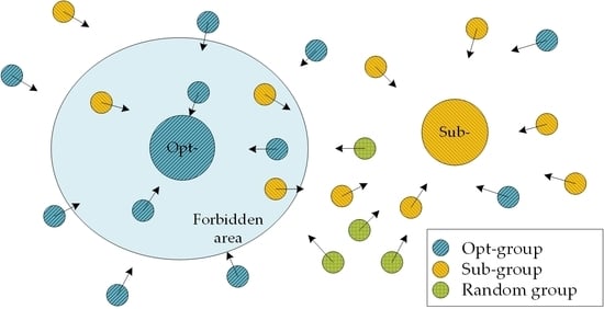
Based on the standard PSO shown in Figure 1, the procedure of the mc-PSO is as shown in Figure 3, in which two components are extracted simultaneously.

As shown in Figure 3, when two components are extracted simultaneously, the population of mc-PSO is divided into three constant groups. The first one is the Opt-group, shown as the blue circle, which contains the particle with the G-best position, and its neighborhood is the forbidden area to the Sub-group; the second one is the Sub-group, shown as the yellow circle, in which its G-best particle can be chosen only outside the forbidden area; the third one is the random group, shown as the green circle, which has no best particle and is updated following the optimal or suboptimal group.

3.1. The Features of Mc-PSO

The three groups of the mc-PSO have the following features:

● The independence of groups

The particles in the three groups are relatively fixed, and the particles in the Opt- and Sub-groups update their positions and velocities according to their own L- and G-best parameters to ensure their convergence in every iteration. The random group without a best particle is divided into two subgroups to update their parameters following the Opt- and Sub-groups, and once the fitness value of a particle is higher than the smallest one in the other two groups, the smallest one could be replaced by the higher one in the random group. Of course, the number of replaced particles is restricted to enhance the whole population’s randomness when exchanging the information among the three groups.

● The strength of the optimal group

Although the aim of mc-PSO is to extract several components simultaneously, the global and stable convergence of the algorithm is more important. The G-best particle in the Opt-group is the best one of the whole population, and its neighborhood is the area forbidden to the Sub-group’s G-best particle, while the particles in the Sub-group could achieve a position in the forbidden area, but their G-best particle must be chosen outside this area, by which means their parameters are subject to updating and searching for the suboptimal solutions only.

● The opportunity of the suboptimal group

If a particle in the Sub-group gets the G-best fitness of the whole population, the Sub- and the Opt-group are exchanged with each other, and in the next iteration, the Opt-group becomes the Sub-group, and vice versa.

● The limitation of the suboptimal group

When a particle of the Sub-group enters into the forbidden area, it may have a relatively high fitness value. However, its best result is only a repetition of the G-best solution in the Opt-group, unless its fitness is greater than the G-best particle and the two groups exchange with each other. Because of the forbidden area, the G-best particle in the Sub-group does not have the highest fitness of the whole population, while the other particles in the Sub-group are attracted to gather around the suboptimal solution.

3.2. The Procedure of the Mc-PSO Algorithm

According to the TF decomposing process of mc-PPS, the searching parameters are the polynomial phase parameters over 2 orders, while the fitness is the maximum spectrum value of the phase-compensated signal, and the position of the maximum value, i.e., $a_1$ of the PPS is actually the azimuth position of the scattering center. Therefore, in the mc-PSO algorithm, the forbidden area of the optimal particle can be set based on the position of the scattering center, by which the Opt- and Sub-groups are distinguished. The procedure of the mc-PSO algorithm applied in FDE–AJTF decomposition is as shown in Figure 4.

As shown in Figure 4, the procedure is as follows:

(a)

Set the neighborhood range of the forbidden area, $D_{\mathrm{neighbor}}$, and initialize the first population $P_1$ and the iteration $g=1$;

(b)

Divide the population into three groups, $P_1=\left\{P_{1,{\mathrm{sub}}_1},P_{1,{\mathrm{sub}}_2},P_{1,{\mathrm{sub}}_3}\right\}$, where $P_{1,{\mathrm{sub}}_1}$ is the Opt-group, $P_{1,{\mathrm{sub}}_2}$ is the Sub-group, and $P_{1,{\mathrm{sub}}_3}$ is the random group.

(c)

In the gth iteration, search for the G-best fitness value ${F_{\mathrm{G},g}|}_{{\mathrm{sub}}_1}$ of the Opt-group, update the particle with the G-best position ${P_{\mathrm{G},g}|}_{{\mathrm{sub}}_1}$, search for the position ${X_{\mathrm{G},g}|}_{{\mathrm{sub}}_1}$ of the responding scattering center, and set the neighborhood of ${X_{\mathrm{G},g}|}_{{\mathrm{sub}}_1}$ as the forbidden area of the Sub-group.

(d)

Search for the G-best fitness value ${F_{\mathrm{G},g}|}_{{\mathrm{sub}}_2}$ of the Sub-group, update the particle with the G-best position ${P_{\mathrm{G},g}|}_{{\mathrm{sub}}_2}$, and search for the position ${X_{\mathrm{G},g}|}_{{\mathrm{sub}}_2}$ of the responding scattering center, while ${X_{\mathrm{G},g}|}_{{\mathrm{sub}}_2}$ is chosen only out of the neighborhood of ${X_{\mathrm{G},g}|}_{{\mathrm{sub}}_1}$, as follows:

$${P_{\mathrm{G},g}|}_{{\mathrm{sub}}_2}=\arg \max \left({\left\{F_{\mathrm{L},g,m^{\prime }}\right\}|}_{{\mathrm{sub}}_2}\right)$$

(20)

where $m^{\prime }$ is the particle number in the Sub-group whose position is outside the forbidden area, and ${P_{\mathrm{L},g,m^{\prime }}|}_{{\mathrm{sub}}_2}$ conforms to the following equation:

$$\begin{array}{ccc}{P_{\mathrm{L},g,m^{\prime }}|}_{{\mathrm{sub}}_2}& s.t.& \left|{X_{\mathrm{L},g,m^{\prime }}|}_{{\mathrm{sub}}_2}-{X_{\mathrm{G},g}|}_{{\mathrm{sub}}_1}\right|>D_{\mathrm{neibor}}\end{array}$$

(21)

where $D_{\mathrm{neighbor}}$ is the neighborhood range.

(e)

Set the L-best fitness of the particles of the Sub-group in the forbidden area ${F_{\mathrm{fitL},g,m^{″}}|}_{{\mathrm{sub}}_2}$ to zero, as follows:

$${F_{\mathrm{L},g,m^{″}}|}_{{\mathrm{sub}}_2}=0\begin{array}{ccc}& if& \end{array}\left|{X_{\mathrm{L},g,m^{″}}|}_{{\mathrm{sub}}_2}-{X_{\mathrm{G},g}|}_{{\mathrm{sub}}_1}\right|\le D_{\mathrm{neibor}}$$

(22)

where $m^{″}$ is the particle number of the Sub-group in the forbidden area.

The parameters and the fitness of the particles in the forbidden area would definitely be updated and step out the forbidden area. The manipulation ensures the suboptimal group does not include the best solution of the Opt-group and thus avoids invalid searching.

(f)

Divide the random group into two subgroups, $P_{g,{\mathrm{sub}}_3}=\left\{P_{g,{\mathrm{sub}}_{31}},P_{g,{\mathrm{sub}}_{32}}\right\}$, and attach to the end of the Opt- and Sub-groups, respectively, to compose two mixed groups $\left\{P_{g,{\mathrm{sub}}_1},P_{g,{\mathrm{sub}}_{31}}\right\}$ and $\left\{P_{g,{\mathrm{sub}}_2},P_{g,{\mathrm{sub}}_{32}}\right\}$, and then update their parameters using ${P_{\mathrm{G},g}|}_{{\mathrm{sub}}_1}$ and ${P_{\mathrm{G},g}|}_{{\mathrm{sub}}_2}$, respectively.

(g)

Update the two mixed groups, $\left\{{\mathbf{P}}_{g,{\mathrm{sub}}_1}^{\mathbf{\prime }},{\mathbf{P}}_{g,{\mathrm{sub}}_{31}}^{\mathbf{\prime }}\right\}$ and $\left\{{\mathbf{P}}_{g,{\mathrm{sub}}_2}^{\mathbf{\prime }},{\mathbf{P}}_{g,{\mathrm{sub}}_{32}}^{\mathbf{\prime }}\right\}$, calculate their fitness $F_{g,m}^{\prime }$ and the scattering position $X_{g,m}^{\prime }$, and update their L-best value $F_{\mathrm{L},g,m}^{\prime }$ and position $P_{\mathrm{L},g,m}^{\prime }$.

(h)

In the first mixed group $\left\{{\mathbf{P}}_{g,{\mathrm{sub}}_1}^{\mathbf{\prime }},{\mathbf{P}}_{g,{\mathrm{sub}}_{31}}^{\mathbf{\prime }}\right\}$, if the maximum fitness value in the random subgroup ${\mathbf{P}}_{g,{\mathrm{sub}}_{31}}^{\mathbf{\prime }}$ is larger than the minimum fitness value in the Opt-group ${\mathbf{P}}_{g,{\mathrm{sub}}_1}^{\mathbf{\prime }}$, exchange the two respective particles as follows:

$${P_{g,m_1}^{\prime }|}_{{\mathrm{sub}}_1}\iff {P_{g,m_2}^{\prime }|}_{{\mathrm{sub}}_{31}}\begin{array}{ccc}& if& \end{array}{F_{\mathrm{L},g,m_1}^{\prime }|}_{{\mathrm{sub}}_1}\le {F_{\mathrm{L},g,m_2}^{\prime }|}_{{\mathrm{sub}}_{31}}$$

(23)

where the symbol $\iff$ means exchanging the two particles’ groups; $m_1$ is the particle number with the minimum fitness value in the Opt-group ${\mathbf{P}}_{g,{\mathrm{sub}}_1}^{\mathbf{\prime }}$; and $m_2$ is the particle number with the maximum fitness value in the random subgroup ${\mathbf{P}}_{g,{\mathrm{sub}}_{31}}^{\mathbf{\prime }}$, as follows:

$$\{\begin{array}{c}{F_{\mathrm{L},g,m_1}^{\prime }|}_{{\mathrm{sub}}_1}=\min \left({\left\{F_{\mathrm{L},g,m}^{\prime }\right\}|}_{{\mathrm{sub}}_1}\right)\\ {F_{\mathrm{L},g,m_2}^{\prime }|}_{{\mathrm{sub}}_{31}}=\max \left({\left\{F_{\mathrm{L},g,m}^{\prime }\right\}|}_{{\mathrm{sub}}_{31}}\right)\end{array}$$

(24)

Then, apply the same processing to the second mixed group, $\left\{{\mathbf{P}}_{g,{\mathrm{sub}}_2}^{\mathbf{\prime }},{\mathbf{P}}_{g,{\mathrm{sub}}_{32}}^{\mathbf{\prime }}\right\}$.

Only one pair of particles are exchanged in each mixed group, the purpose of which is to maintain the relative independence of the Opt- and Sub-groups and to maintain the randomness of the random group.

(i)

If the G-best fitness of the Sub-group is larger than that of the Opt-group, exchange the roles of the two groups, as follows:

$${\mathbf{P}}_{g,{\mathrm{sub}}_1}^{\mathbf{\prime }}\iff {\mathbf{P}}_{g,{\mathrm{sub}}_2}^{\mathbf{\prime }}\begin{array}{ccc}& if& \end{array}{F_{\mathrm{L},g,m_1}^{\prime }|}_{{\mathrm{sub}}_1}<{F_{\mathrm{L},g,m_2}^{\prime }|}_{{\mathrm{sub}}_2}$$

(25)

where the symbol $\iff$ means exchanging the two groups; and $m_1$ and $m_2$ are the particle numbers with maximum fitness in the Opt- and Sub-groups, respectively.

$$\{\begin{array}{c}{F_{\mathrm{L},g,m_1}^{\prime }|}_{{\mathrm{sub}}_1}=\max \left({\left\{F_{\mathrm{L},g,m}^{\prime }\right\}|}_{{\mathrm{sub}}_1}\right)\\ {F_{\mathrm{L},g,m_2}^{\prime }|}_{{\mathrm{sub}}_2}=\max \left({\left\{F_{\mathrm{L},g,m}^{\prime }\right\}|}_{{\mathrm{sub}}_2}\right)\end{array}$$

(26)

(j)

The three groups $\left\{{\mathbf{P}}_{g,{\mathrm{sub}}_1}^{\mathbf{\prime }},{\mathbf{P}}_{g,{\mathrm{sub}}_2}^{\mathbf{\prime }},{\mathbf{P}}_{g,{\mathrm{sub}}_3}^{\mathbf{\prime }}\right\}$ become the (g + 1)th population, $P_{g+1}=\left\{P_{g+1,{\mathrm{sub}}_1},P_{g+1,{\mathrm{sub}}_2},P_{g+1,{\mathrm{sub}}_3}\right\}$, and determine whether the stop condition is met; if it is, perform step (k), and if not, update the iteration $g=g+1$ and perform step (c).

(k)

Output the G-best parameters ${P_{\mathrm{G},g}|}_{{\mathrm{sub}}_1}$ and ${P_{\mathrm{G},g}|}_{{\mathrm{sub}}_2}$ of the Opt- and Sub-groups, respectively, and the algorithm is completed.

3.3. The Effectiveness of Suboptimal Component

Two components are outputted for each completion of the mc-PSO algorithm. However, if only one efficient component is left in the signal, the second component is invalid, so the effectiveness of the suboptimal component should be judged. According to the feature of the mc-PPS signal, the two real components are independent to each other and one’s extraction cannot affect the other; otherwise, extracting a component would severely affect the fitness of the other.

Therefore, if the fitness of the optimal and suboptimal solutions are $F_1$ and $F_2$, respectively, and the fitness of the suboptimal solution after the optimal component is extracted is $F_2^{\prime }$, the ratio of the two fitness values $F_2$ and $F_2^{\prime }$ before and after the optimal component is extracted can judge the effectiveness of the suboptimal solution, as follows:

$$\{\begin{array}{l}\mathrm{Effective},\begin{array}{cc}& \end{array}{R}_{\mathrm{fit}}\ge H_{\mathrm{fit}}\\ \mathrm{Ineffective},\begin{array}{cc}& otherwise\end{array}\end{array},\begin{array}{cc}& \end{array}{R}_{\mathrm{fit}}=\frac{F_2^{\prime }}{F_2}$$

(27)

where $R_{\mathrm{fit}}$ is the fitness ratio and $H_{\mathrm{fit}}$ is the threshold. If the suboptimal solution is not a real component, the fitness $F_2^{\prime }$ would be obviously lower than $F_2$. To ensure the effectiveness of every component, the threshold can be set as $H_{\mathrm{fit}}=0.99$.

4. Simulation and Test

To analyze the convergence, accuracy, and computation of the mc-PSO, several simulations are performed and the comparisons between mc-PSO and GA, DE, and standard PSO are made. The simulated data is contained in four four-order PPS components with 500 points within the time −0.5~0.5 s, as

Table 1. The parameters of PPS components.

	$\mathbf{A}$	${\mathbf{a}}_1$	${\mathbf{a}}_2$	${\mathbf{a}}_3$	${\mathbf{a}}_4$	${\mathsf{\tau }}_{\mathbf{s}}$	${\mathsf{\tau }}_{\mathbf{d}}$	${\mathbf{R}}_{\mathbf{E}}$
Component 1	2.0	32.1	55.6	212.4	10.1	−0.5	0.5	46.30%
Component 2	1.6	398.2	156.6	−149.3	−20.2	−0.5	0.4	29.63%
Component 3	1.2	333.9	−98.2	−102.2	30.7	−0.4	0.5	16.67%
Component 4	0.8	262.8	−23.1	−91.5	−10.8	−0.5	0.5	7.41%

shows.

The parameters of the four optimal algorithms are set as in

Table 2. The parameters of the four optimal algorithms.

GA		DE		Standard PSO		mc-PSO
Individual number	100~500	Individual number	100~500	Particle number	100~500	Particle number	100~500
Iteration	500	Iteration	500	Iteration	500	Iteration	500
Choose probability	0.8	Mutation factor	0.4	Constraint factor	0.729	Components once extraction	2
Cross probability	0.5	Cross probability	0.7	Attraction factor	1.496	Neighborhood range	30

, in which the main variable is the number of individuals or particles, and the other parameters are optimal empirical values obtained after many simulation experiments.

The time frequency distribution (TFD) of the simulated data obtained by short time Fourier transform (STFT) is shown in Figure 5, and the time frequency representation (TFR) obtained by FDE–AJTF decomposition with four different optimal algorithms is shown in Figure 6.

As shown in Figure 5, the general trend of the signal is obtained with low resolution by STFT, while in Figure 6, the four components were extracted by FDE–AJTF decomposition with higher resolutions. Furthermore, the four TFRs obtained by FDE–AJTF decomposition with different optimal algorithms are almost the same as each other, which indicates that the four TFRs correspond with the simulated signal generated as shown in Table 1, and all the four optimal algorithms can satisfy the requirement of FDE–AJTF decomposition for mc-PPS signal.

4.1. Convergence

To get the statistical characteristics of the four optimal algorithms, a Monte Carlo test was carried out in each simulation for 500 times. The convergences of the four optimal algorithms can be expressed by the change curves of the best fitness in the population. When the first component was extracted, the four algorithms’ change curves of the best fitness with the iteration were as shown in Figure 7, Figure 8, Figure 9 and Figure 10.

As shown in Figure 7, Figure 8, Figure 9 and Figure 10, the best fitness values of the four algorithms converge to one or two values with increasing iterations, and the converging speed becomes faster with the increasing number of individuals. In Figure 7, it is evident that some solutions of the GA algorithm fall into a local optimal solution and, in Figure 9, the PSO has the fastest convergence speed and a few solutions fall into a local optimal solution, while in Figure 8, the DE algorithm has the best convergence, but the slowest speed. As shown in Figure 10, two solutions are obtained in the mc-PSO algorithm with good convergence, so even though its convergence speed is slower than the standard PSO, the searching times are reduced by half compared to the standard PSO.

Furthermore, in the worst case, the convergence of the mc-PSO is as the same as the standard PSO because of former one’s procedure in Figure 4. Moreover, the lower convergence of the standard PSO is mainly caused by its local optimal solution, while in mc-PSO, when a local optimal solution is obtained by the Opt-group, the Sub-group has to search another solution out of the neighborhood of the local optimal solution, so the suboptimal solution would be the global optimal solution of the whole population. Then, in step (i) of the processing procedure, the roles of the two groups will be exchanged, finally the global optimal solution is obtained. As a result of that, the probability of correctly extracting the global optimal solution is increased by the two divided groups in the mc-PSO, and its convergence is enhanced as shown in Figure 9 and Figure 10.

4.2. Accuracy

The accuracies of the four algorithms can be expressed by the probability of correctly extracting the first component, which can be expressed by the ratio of the individuals with the best fitness of the whole population. The accuracies of the four algorithms are shown in Figure 11, Figure 12, Figure 13 and Figure 14 and

Table 3. The probabilities of correctly extracting the first component of the four algorithms.

Individuals	GA	DE	STD PSO	mc-PSO
				1st CMPT	2nd CMPT
200	81.5%	100%	98.0%	99.0%	99.0%
300	91.0%	100%	99.0%	99.5%	99.0%
400	91.0%	100%	99.0%	100%	99.5%
500	91.0%	100%	99.0%	100%	100%

.

As shown in Table 3 and Figure 11, when 400 individuals are present, the GA’s probability of correctly extracting the first component is 91%, and in Figure 13, the PSO’s is 99%, and when only 200 individuals are present, the DE’s accuracy is already 100%. It is evident that the DE algorithm has the best accuracy and stability, those of the PSO are worse than the DE, and the GA has the worst. As shown in Figure 14, when 500 individuals are present in the mc-PSO algorithm, the probabilities of correctly extracting the first and the second components are both 100%, which indicates that its accuracy is better than the standard PSO and its stability is improved.

4.3. Computation

Due to the extraction error in the mc-PSO algorithm, having two components in one extraction may be not both effective, and more than two extractions may be needed to extract four components. The average number of extractions it needs to search for and extract four components is shown in Figure 15.

As shown in Figure 15, the average number of extractions is about 2.2, which indicates that the effectiveness judgment condition detailed in Section 3.3 is effective and the components’ effectiveness is ensured.

According to the detailed procedures of the four algorithms, the computations in every iteration are mainly from the individuals’ fitness update, which requires the Fourier transform. Therefore, the whole computation of the four algorithms can be expressed by their FFT operation times, which are shown in

Table 4. The computation of the four algorithms.

	GA	DE	PSO	mc-PSO
Number of individuals	400	300	400	400
Iteration	400	400	200	300
Number of extractions	4	4	4	2.2
Number of fitness updates	640,000	480,000	320,000	264,000

. The simulation environment is shown in

Table 5. The simulation environment.

Items	Parameters
CPU	Xeon E3 2.9 GHz
Cores	4 Cores and 8 Threads
Memory	64 GB
Disk	1 T SSD
Software	Matlab R2016b
Monte Carlo times	500

, and the normalized computing time is shown in Figure 16.

As shown in Table 4, the mc-PSO has the least fitness update times of the four algorithms, which corresponds to the normalized theoretical value in Figure 16, and the simulation time conforms to the theoretical value. It is evident that the mc-PSO has the lowest computational requirements and the shortest operation time, which confers about 30% improvement compared to the standard PSO algorithm.

5. Conclusions

The echo of maneuvering targets can be expressed as a multicomponent polynomial phase signal (mc-PPS), which should be processed by time frequency analysis methods. The FDE–AJTF decomposition is an effective method to correctly search for and extract the components of the mc-PPS signal. However, a difficult problem of the FDE–AJTF decomposition is searching for the optimal parameters in the solution space, which is essentially a multidimensional optimization problem with different extremal solutions. Although the PSO is an efficient and widely-used optimal algorithm, on one hand, it has disadvantages that easily fall into the local optimal solution; on the other hand, its feature makes extracting several components simultaneously possible.

In this paper, based on the feature of the standard PSO, a novel mc-PSO algorithm is presented to solve the multidimensional optimization problem, which has the new characteristic that can extract several components simultaneously. To achieve the purpose, the population of the mc-PSO is divided into three groups, i.e., optimal, suboptimal, and random groups, while the neighborhood of the best particle in the Opt-group is set as the forbidden area for the Sub-group, and then two different independent components can be extracted in one extraction by the Opt- and Sub-group, respectively.

Three simulation tests are carried out and compared with the standard PSO, GA, and DE algorithms, the performances in convergence, accuracy, and computation of the mc-PSO are analyzed. According to the test results, the GA has the worst performance in all three aspects; the DE algorithm has the best convergence and accuracy, but the slower speed; the standard PSO has the faster speed but worse convergence and accuracy than DE; the presented mc-PSO algorithm has the fastest speed and comparable convergence and accuracy with DE. As concluded, it is verified that the mc-PSO has the best performance and that the convergence, accuracy, and stability are improved, while its searching times and computation are reduced.

The real-time application is the eventual goal of an optimal algorithm; however, although the computation is reduced and the convergence speed is improved, the mc-PSO is hardly used in real-time applications yet, especially in high-resolution signal processing with large data. In the follow-up research, the real-time processing application of the mc-PSO or other optimal algorithms will be the direction and focus.

References

- Lao, G.; Yin, C.; Ye, W.; Sun, Y.; Li, G. A frequency domain extraction based adaptive joint time frequency decomposition method of maneuvering target radar echo. Remote Sens. 2018, 10, 266. [Google Scholar] [CrossRef]
- Chen, V.C.; Li, F.; Ho, S.S.; Wechsler, H. Micro-Doppler effect in radar: Phenomenon, model, and simulation study. IEEE Trans. Aerosp. Electr. Syst. 2006, 42, 2–21. [Google Scholar] [CrossRef]
- Lao, G.; Liu, G.; Wu, X. The modeling and simulation of spaceborne SAR moving vessel imaging based on Matlab class. In Proceedings of the International Conference on Frontiers of Manufacturing Science and Measuring Technology (FMSMT), Taiyuan, China, 24–25 June 2017; Atlantis Press: Paris, France, 2017; Volume 130, pp. 1583–1586, ISBN 978-94-6252-331-9. [Google Scholar]
- Lao, G.; Yin, C.; Ye, W.; Sun, Y.; Li, G.; Han, L. An SAR-ISAR Hybrid Imaging Method for Ship Targets Based on FDE–AJTF Decomposition. Electronics 2018, 7, 46. [Google Scholar] [CrossRef]
- Peleg, S.; Porat, B. Estimation and classification of polynomial-phase signals. IEEE Trans. Inf. Theory 1991, 37, 422–430. [Google Scholar] [CrossRef]
- Wang, Y.; Abdelkader, A.C.; Zhao, B.; Wang, J. ISAR imaging of maneuvering targets based on the modified discrete polynomial-phase transform. Sensors 2015, 15, 22401–22418. [Google Scholar] [CrossRef] [PubMed]
- Jing, F.; Si, W.; Jiao, S. A hybrid LVD-HAF method of quadratic frequency-modulated signals. In Proceedings of the Applied Computational Electromagnetics Society Symposium—Italy (ACES), Florence, Italy, 26–30 March 2017; ISBN 978-1-5090-5335-3. [Google Scholar]
- Zheng, J.; Su, T.; Zhu, W.; Zhang, L.; Liu, Z.; Liu, Q. ISAR imaging of nonuniformly rotating target based on a fast parameter estimation algorithm of cubic phase signal. IEEE Trans. Geosci. Remote Sens. 2015, 53, 4727–4740. [Google Scholar] [CrossRef]
- Popovica, V.; Djurovica, I.; Stankovica, L.; Thayaparanb, T.; Dakovica, M. Autofocusing of SAR images based on parameters estimated from the PHAF. Signal Process. 2010, 90, 1382–1391. [Google Scholar] [CrossRef]
- Kulkarni, R.; Rastogi, P. Multiple phase estimation in digital holographic interferometry using product cubic phase function. Opt. Lasers Eng. 2013, 51, 1168–1172. [Google Scholar] [CrossRef]
- Djurovic, I.; Simeunovic, M.; Wang, P. Cubic Phase Function: A Simple Solution to Polynomial Phase Signal Analysis. Elsevier Signal Process. 2017, 135, 48–66. [Google Scholar] [CrossRef]
- Friedlander, B.; Francos, J.M. Estimation of amplitude and phase parameters of multicomponent signals. IEEE Trans. Signal Process. 1995, 43, 917–926. [Google Scholar] [CrossRef]
- Djurovic, I.; Stankovic, L. Quasi maximum likelihood estimator of polynomial phase signals. IET Signal Process 2014, 13, 347–359. [Google Scholar] [CrossRef]
- Djurovic, I.; Simeunovic, M. Review of the quasi-maximum likelihood estimator for polynomial phase signals. Dig. Signal Process. 2018, 72, 59–74. [Google Scholar] [CrossRef]
- Trintinalia, L.; Ling, H. Joint time-frequency ISAR using adaptive processing. IEEE Trans. Antennas Propag. 1997, 45, 221–227. [Google Scholar] [CrossRef]
- Thayaparan, T.; Brinkman, W.; Lampropoulos, G. Inverse synthetic aperture radar image focusing using fast adaptive joint time–frequency and three-dimensional motion detection on experimental radar data. IET Signal Process. 2010, 4, 382–394. [Google Scholar] [CrossRef]
- Brinkman, W.; Thayaparan, T. Focusing inverse synthetic aperture radar images with higher-order motion error using the adaptive joint-time-frequency algorithm optimised with the genetic algorithm and the particle swarm optimisation algorithm-comparison and results. IET Signal Process. 2010, 4, 329–342. [Google Scholar] [CrossRef]
- Li, Y.; Fu, Y.; Li, X.; Lewei, L. ISAR imaging of multiple targets using particle swarm optimization—Adaptive joint time frequency approach. IET Signal Process. 2010, 4, 343–351. [Google Scholar] [CrossRef]
- Garcíagonzalo, E.; Fernándezmartínez, J.L. A Brief Historical Review of Particle Swarm Optimization (PSO). J. Bioinform. Intell. Control 2012, 1, 3–16. [Google Scholar] [CrossRef]
Figure 1.
The schematic diagram of particle swarm optimization (PSO).
Figure 2.
The schematic diagram of PSO.
Figure 3.
The schematic diagram of mc-PSO.
Figure 4.
The procedure of mc-PSO applied in FDE–AJTF decomposition.
Figure 5.
TFD obtained by STFT.
Figure 6.
TFRs obtained by four algorithms: (a) GA, (b) DE, (c) standard PSO, and (d) mc-PSO.
Figure 7.
The best fitness change curves of GA with different numbers of individuals: (a) 200 individuals; (b) 300 individuals; and (c) 400 individuals.
Figure 8.
The best fitness change curves of DE with different numbers of individuals: (a) 200 individuals; (b) 300 individuals; and (c) 400 individuals.
Figure 9.
The best fitness change curves of standard PSO with different numbers of individuals: (a) 200 individuals; (b) 300 individuals; and (c) 400 individuals.
Figure 10.
The best fitness change curves of mc-PSO with different numbers of individuals: (a) 300 individuals; (b) 400 individuals; and (c) 500 individuals.
Figure 11.
The probability of correctly extracting the first component of GA with different numbers of individuals: (a) 200 individuals; (b) 300 individuals; and (c) 400 individuals.
Figure 12.
The probability of correctly extracting the first component of DE with different number of individuals: (a) 200 individuals; (b) 300 individuals; and (c) 400 individuals.
Figure 13.
The probability of correctly extracting the first component of standard PSO with different number of individuals: (a) 200 individuals; (b) 300 individuals; and (c) 400 individuals.
Figure 14.
The probability of correctly extracting the first and second components of mc-PSO with different number of individuals: (a) 300 individuals; (b) 400 individuals; and (c) 500 individuals.
Figure 15.
The average times of searching for and extracting four components with the mc-PSO.
Figure 16.
The normalized computing time of the four algorithms.