1. Introduction and Motivation
The extensive volume of patient medical data recorded at every moment in hospitals, medical imaging centers and other medical organizations has become a major issue. The need for quasi-infinite storage space and efficient real-time transmission in specific applications such as medical imaging, military imaging and satellite imaging requires advanced techniques and technologies including coding methods to reduce the amount of data to be stored or transmitted. Without coding of information, it is very difficult and sometimes impossible to make a way to store or communicate big data (large volumes of high velocity and complex images, audio and video information) via the internet. The encoding of these data is obtained by eliminating the redundant or unnecessary information in the original frame which cannot be identified with the naked eye.
Telemedicine offers valuable specialty diagnostic services to underserved patients in rural areas, but often requires significant image compression to transmit medical images using limited bandwidth networks. The difficulty is that compressing images such as those for tele-echography can introduce artifacts and reduce medical image quality which affects directly the diagnosis [
1].
This possible disadvantage is inherent in all lossy compression methods.
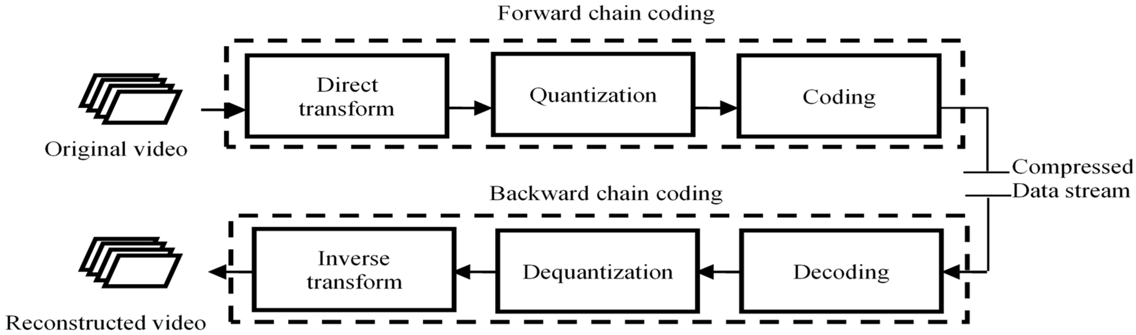
Figure 1 recalls the key steps of video coding. Transformation is a linear and reversible operation that allows the image to be represented in the transform domain where the useful information is well localized. This property will make it possible during the compression to achieve good discrimination, that is to say the suppression of unnecessary or redundant information. The discrete cosine transform and the wavelet transform are among the most popular transforms proposed for image and video coding.
Quantization is the step of the compression process during which a large part of the elimination of unnecessary or redundant information occurs.
Coding techniques e.g., Huffman coding and arithmetic coding [
2], are the best-known entropy coding particularly in image and video coding.
It is well known that lossless compression methods have the advantage of providing an image without any loss of quality and the disadvantage of compressing weakly. Hence, this type of compression is not suitable for transmission or storage of big data such as video. Conversely, lossy compression produces significantly smaller file sizes often at the expense of image quality. However, lossy coding based on transforms has gained great importance when several applications have appeared. In particular, lossy coding represents an acceptable option for coding medical images. e.g., a DICOM (Digital Imaging Communication in Medicine) JPEG (Joint Photographic Experts Group) based on discrete cosine transform (DCT) and a DICOM JPEG 2000 based on wavelet. In this context, wavelet-based image coding, e.g., JPEG2000, using multiresolution analysis [
3,
4] exhibits performance that is highly superior to other methods such as those based on DCT, e.g., JPEG.
In 1993, Shapiro introduced a lossy image compression algorithm that he called embedded zerotrees of wavelet (EZW) [
5]. The success of coding wavelet approaches is largely due to the occurrence of effective sub-band coders. The EZW encoder is the first to provide remarkable distortion-rate performance while allowing progressive decoding of the image. The principle of zerotrees, or other partitioning structures in sets of zeros, makes it possible to take account of the residual dependence of the coefficients between them. More precisely, since the high-energy coefficients are spatially grouped, their position is effectively computed by indicating the position of the sets of low-energy coefficients. After separation of the low-energy coefficients and the energetic coefficients, the latter is relatively independent and can be efficiently coded using quantification and entropy coding techniques.
In 1996, Said and Pearlman proposed a hierarchical tree partitioning coding scheme called set partitioning in hierarchical tree (SPIHT) [
6], based on the same basic EZW, and exhibiting better performance than the original EZW.
Video compression algorithms such as H.264 and MPEG use inter-frame prediction to reduce video data between a series of images. This involves techniques such as differential coding where an image is compared with a reference image and only the pixels that have changed with respect to that reference image are coded.
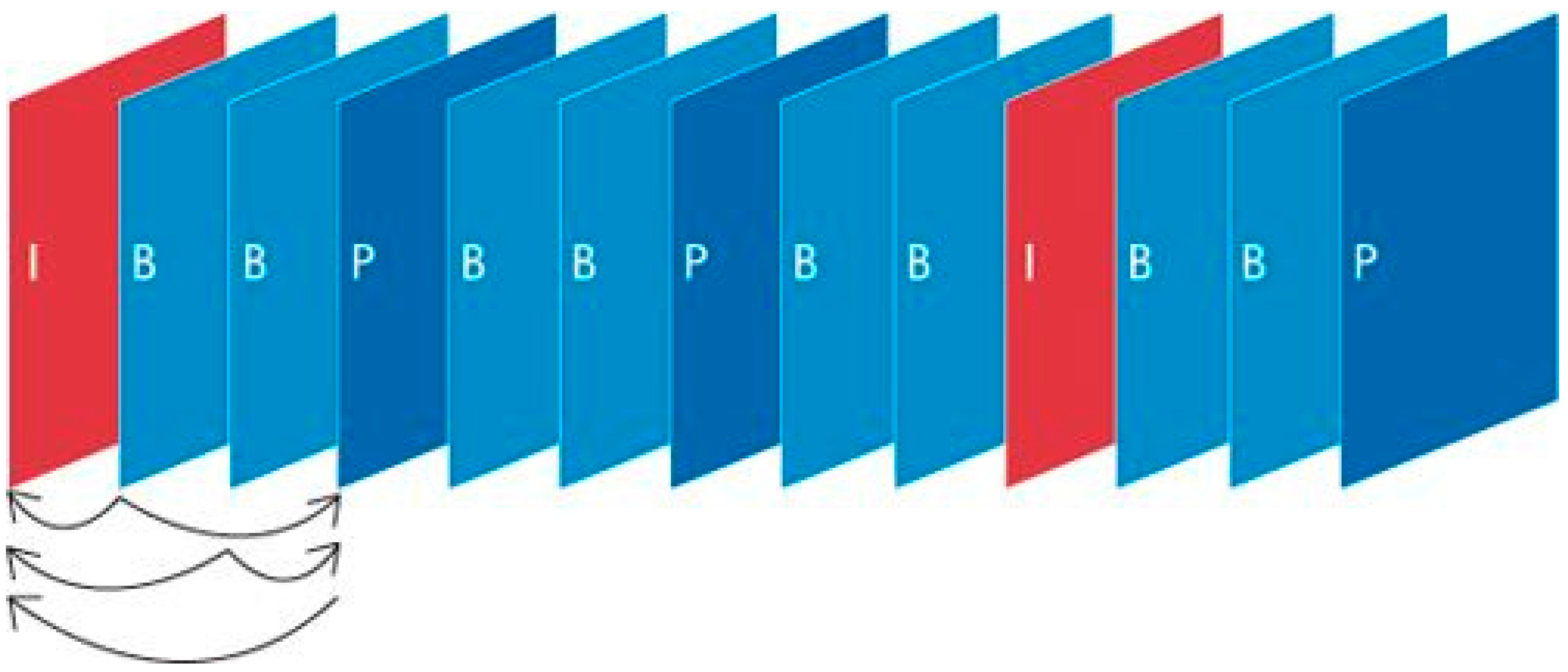
MPEG (Moving Picture Experts Group) allows to encode video using three coding modes:
Intra coded frames (I): frames are coded separately without reference to previous images (i.e., as JPEG coding).
Predictive coded frames (P): images are described by difference from previous images.
Bidirectionally predictive coded frames (B): the images are described by difference with the previous image and the following image.
In order to optimize MPEG coding, the image sequences are in practice coded in a series of I, B, and P images, the order of which has been determined experimentally. The typical sequence called GOP (group of pictures) is as follows (see
Figure 2):
To evaluate the visual quality of the reconstructed video, several measurements of the quality of the MPEG video are validated in [
7,
8].
As a successor to the famous H.264 or MPEG-4 Part 10 standards [
9,
10], HEVC (High-Efficiency Video Coding) or H.265 standard has recently been defined as a promising standard for video coding, In June 2013 [
11], the first version of HEVC was announced, and to improve the efficiency of the coding of this standard, a set of its components requires more development. In addition, this new system requires new hardware and software investments delaying its adoption in applications such as in the medical field.
In our case, the use of wavelets enhances the contours, which minimizes the impact of information loss in medical imaging, mainly in tumor detection [
12,
13,
14,
15]. Moreover, bandelets are 2nd-generation wavelets and the corresponding transform is an orthogonal multi-resolution transform that is able to capture the geometric content of images and surfaces. Hence, the possible presence of artifacts will be considerably reduced.
Our motivation lies in the prospect of offering a new codec that is simple to implement with performances superior to the current H.264 standard and which could compete with the H.265 or HEVC standard for some applications. This superiority is based on the SPIHT algorithm and the second-generation wavelets.
One can ask: “Why using second generation wavelets (instead of classical wavelets)?”
This new generation of wavelets makes it possible to generate decorrelated coefficients, and to eliminate any redundancy by retaining only the necessary information and it is better suited to geometric data (ridges, contours, curves, or singularities). This 2nd-generation wavelet consists of Xlets such as shearlets, bandelets, curvelets, contourlets, ridgelets, noiselets, etc. These Xlets provide an interesting performance in some applications, e.g., contourlets-based denoising [
16], contourlets-based video coding [
17,
18], curvelets-based contrast enhancement [
19], bandelets-based geometric image representations [
20], shearlets-based image denoising [
21], …
In this paper, we analyse and compare to the current state-of-the-art coding methods, the performances of a new coding method based on bandelet transform where its coefficients are encoded using the set partitioning in hierarchical trees (SPIHT).
The remainder of this paper is organized as follows:
Section 2 presents and recalls the main properties of bandelet transform.
Section 3 introduces bandelet-SPIHT-based video coding.
Section 4 focuses on the experimental aspect and the analysis of the results. It is worth noting that this work is an extension of the conference paper (IECON 2016—42nd Annual Conference of the IEEE Industrial Electronics Society) entitled “Towards a New Standard in Medical Video Compression” [
22]. Compared to this conference paper, there are substantial differences, in this revised version, including large databases used benchmarking and the introduction of HEVC which is the most recent standardized video compression technology. Finally,
Section 5 concludes this study.
2. Bandelet Transform Algorithm
This section describes the different steps of the bandelet approximation algorithm. This algorithm was originally proposed by Peyré and Mallat [
23,
24] in the context of geometric image representation.
2.1. Bandelet Transform
Bandelets are 2nd-generation wavelets and the corresponding transform is an orthogonal multi-resolution transform that is able to capture the geometric content of images and surfaces.
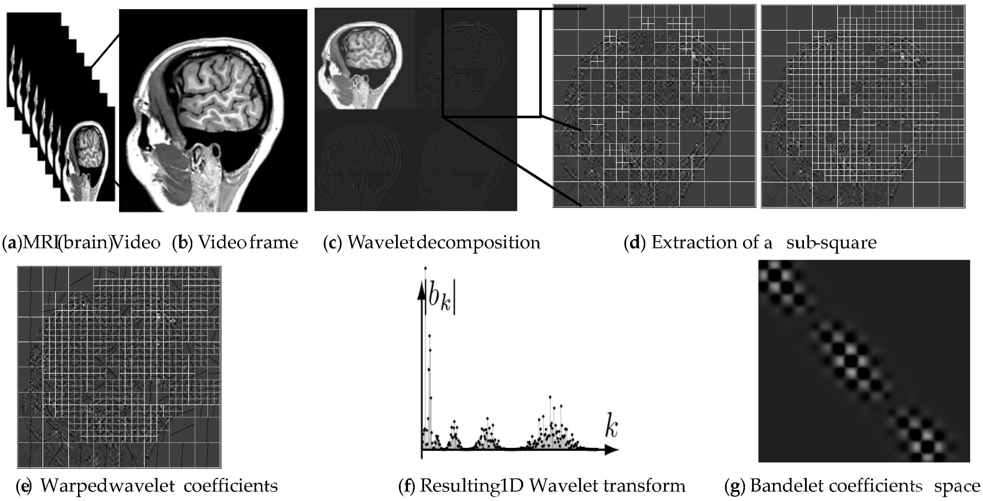
Bandelet transform is carried out as follows:
First, using orthogonal or bi-orthogonal wavelet, we calculate the wavelet transform of the original medical image.
Second, to construct a bandelet basis on the whole wavelet domain, we use a quadtree segmentation at each wavelet scale in dyadic squares, as shown in
Figure 3 where the main steps for computing bandelet transform are summarized and illustrated on a brain magnetic resonance image (MRI). Note that we define a different quadtree for each scale of the wavelet transform (in
Figure 3 only the quadtree of the finest scale is depicted). More specifically, we use the same quadtree for each of the three orientations of the wavelet transform at fixed scale.
A complete representation in a bandelet basis is thus composed of:
An image segmentation at each scale, defined by a quadtree,
For each dyadic square of the segmentation,
- –
a polynomial flow,
- –
bandelet coefficients.
The MATLAB implementation of bandelet transform is freely available in [
25].
2.2. Geometric Flows
The bandelet bases are based on an association between the wavelet decomposition and an estimation of the image information of geometric character. Instead of describing the image geometry through edges, which are most often ill defined, the image geometry is characterized with a geometric flow of vectors. These vectors give the local directions in which the image has regular variations. Orthogonal bandelet bases are constructed by dividing the image support in regions inside which the geometric flow is parallel. The estimation of the geometry is done by studying the contours present in an image. A contour is then seen as a parametric curve that will be characterized by its tangents. To do this, we look for gradients of significant importance in the frame.
Around each region of frames, the local geometry directions, in which the frame has regular variations in the neighborhood of each pixel, are determined by two-dimensional geometric flow of a vector field.
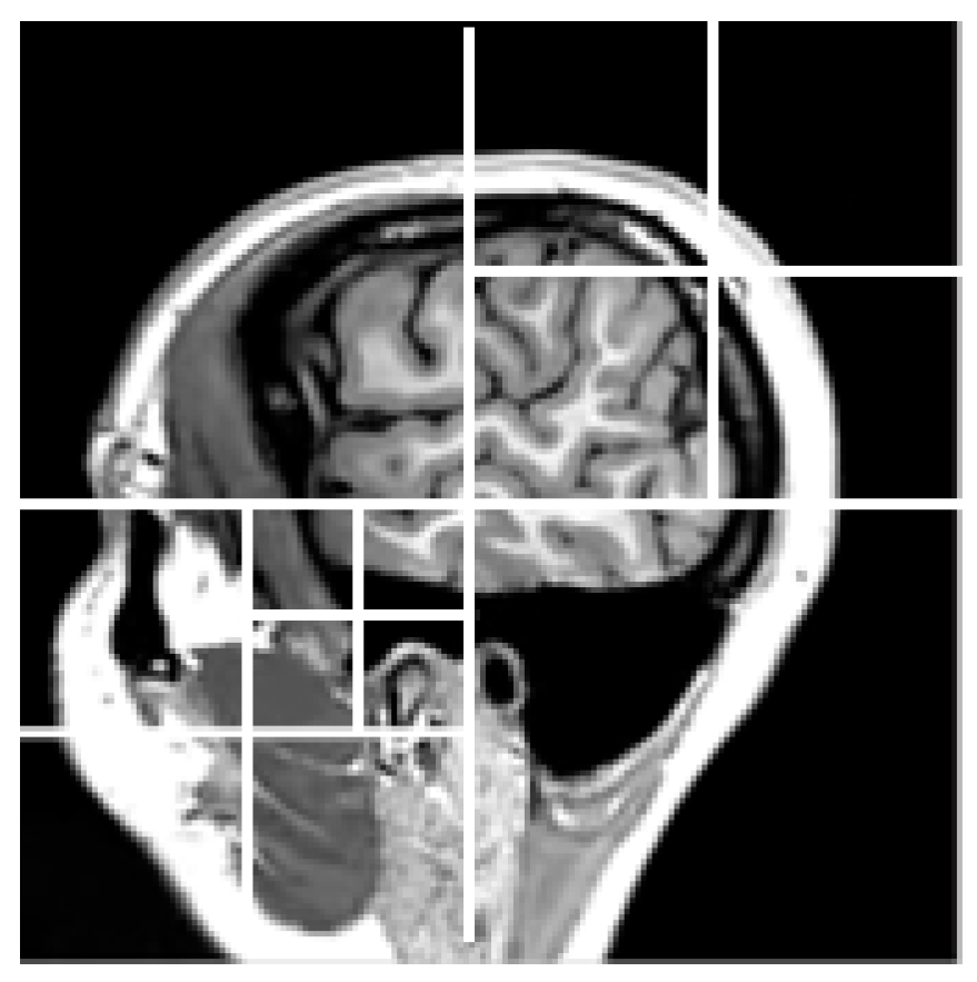
2.3. Quadtree Division Process
In this algorithm, the bandelet transform is performed over each dyadic square and scale in the wavelet domain. This is of course a redundant transform. The best segmentation represented as a quadtree is obtained through Lagrangian optimization. An example of quadtree decomposition is shown in
Figure 4.
In order to minimize the distortion rate, we use a parallel, vertical or horizontal flow in each dyadic square. The macro block is considered regular uniformly and wavelet basis is used if the there is no geometric flow. Otherwise, the sub-block must be processed by warped wavelets, as explained in [
23,
24].
The best quadtree requires a minimization, for each direction, of the following Lagrangian:
where
: Original signal.
: Recovered signal using inverse 1D wavelet transform.
: Number of bits needed to encode the dyadic segmentation.
: Number of bits needed to encode the geometric parameter.
: Number of bits needed to encode the quantized bandelets coefficients.
: Lagrangian multiplier is chosen heuristically to be equal to ¾. To justify this value, see [
20].
: Quantization step.
The following steps implement the quadtree structure.
To compute the quadtree, we first compute the Lagrangian for each dyadic square for the smallest size. Then, the algorithm goes from the smallest size to the biggest, and tries to merge each group of four squares. To do so, it simply computes the Lagrangian of the merged square, and compares it to the sum of the 4 Lagrangians (plus 1 bit, which is the cost of coding a split in the tree).
Using MATLAB code, one can compute a single quadtree for each scale and for each orientation. Sharing the same quadtree for the three orientations leads to a little efficiency increase, at the price of a more complex implementation. The quadtree structure and geometry are stored in an image that is the same size as the original image (and they have the same hierarchical structure as the wavelet transformed image).
2.4. Warped Wavelet along Geometric Flows
In order to perform the complex geometry and remove the redundancy of orthogonal wavelet coefficients, bandelet basis decomposition is applied with a fast application of the geometric flow, quadtree decomposition, warping and bandeletization.
In each dyadic square and at each scale, the geometric flow is used to warp the wavelet basis along the regularity direction. After warping, the next step is to construct bandelets by applying a bandeletization procedure.
The wavelet includes high-pass filters and vanishing moments at lower resolutions, this is valid for vertical and diagonal detail coefficients, but not for horizontal detail coefficients. The problem of regularity along the geometric flow is due to the scaling function where it includes low-pass filters and does not have a vanishing moment at lower resolutions.
To take advantage of regularity along the geometric flow for horizontal detail coefficients, the warped wavelet basis is bandeletized by replacing the horizontal wavelet by modified horizontal wavelet function. Near the singularities, wavelet coefficient correlations are removed by using bandeletization operation.
After warping and bandeletization operations, the regions are regular along the vertical or horizontal direction. In the end, warped wavelets are used to compute bandelet coefficients with 1D discrete wavelet transform than are encoded using SPIHT coder.
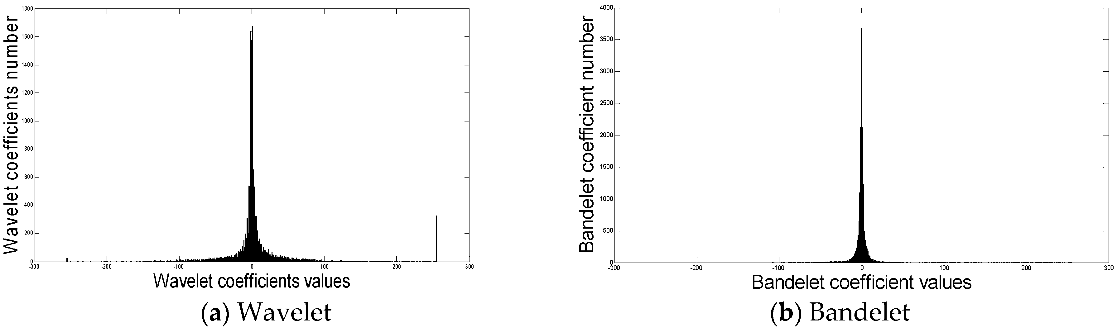
Figure 5 illustrates this feature and compares histograms: wavelet coefficients vs bandelet coefficients.
Figure 5 clearly shows that the bandelet coefficients have larger amplitudes than the wavelet coefficients. This gives the bandelets the ability to carry almost only useful information since what is considered undesirable information is represented by small amplitude coefficients rarely presents in the histogram of bandelet coefficients. Bandelets are, therefore, a natural candidate for effective image compression.
Hence, the SPIHT coder, initially applied to wavelet coefficients, will become bandelet-SPIHT and will be applied to bandelet coefficients: this is what justifies our contribution.
4. Experimental Results and Discussion
We proposed in this work, a new algorithm for medical video coding based on bandelet transform coupled by SPIHT coder that is able to capture complex geometric contents of images and surfaces and reduce drastically existing redundancy in video.
The accuracy of the algorithm is evaluated vs. bit-rate range 0.1 to 0.5 Mbps on sized medical video sequences. Each sequence has variable number of frames, and the frame rate is equal to 30 frames/second.
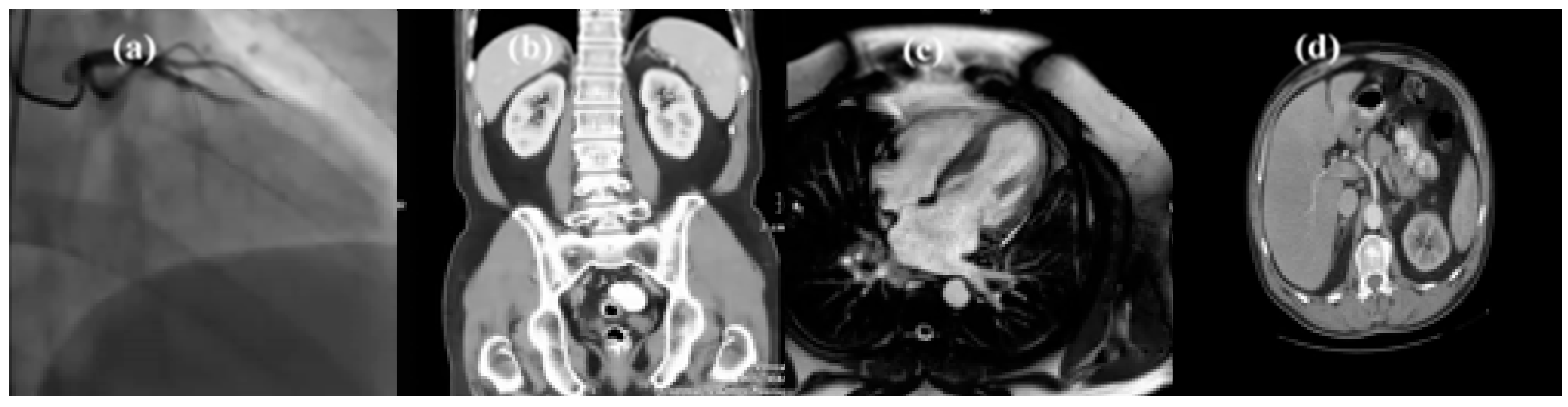
Figure 6 shows a sample of medical frames used for evaluation:
- -
MR imaging is the modality of choice for accurate local staging of bladder cancer (see
Figure 6. (d)). In addition, bladder MR imaging helps detect lymph node involvement. With bladder cancer (T
2-weighted axial image), MRIs are used mainly to look for any signs that cancer has spread beyond the bladder into nearby tissues or lymph nodes.
- -
Cardiac MRI is used to detect or monitor cardiac disease and to evaluate the heart’s anatomy—for example, in the evaluation of congenital heart disease. The MR image of the heart, shown in
Figure 3c, is derived from gradient echo imaging employed in the assessment of ventricular function, blood velocity and flow measurements, assessment of valvular disease, and myocardial perfusion. This MR image is performed with the use of intravenous contrast agents (gadolinium chelates) to enhance the signal of pathology or to better visualize the blood pool or vessels. The paramagnetic effect of gadolinium causes a shortening of T1 relaxation time, thus causing areas with gadolinium to be bright on T1-weighted images. Contrast agent is used in cardiac MRI for evaluation of myocardial perfusion, delayed enhanced imaging (myocardial infarctions, myocarditis, infiltrative processes), differentiation of intracardiac masses (neoplasm vs. thrombus) etc.
- -
Computed tomography (CT) of the abdomen and pelvis, shown in
Figure 3b, is a diagnostic imaging test used to help detect diseases of the small bowel, colon and other internal organs and is often used to determine the cause of unexplained pain. In emergency cases, it can reveal internal injuries and bleeding quickly enough to help save lives.
- -
Figure 3a shows a coronary angiogram showing the left coronary circulation. The exam by coronarography consists in a filmed radiography, typically at 30 frames per second, of coronary (arteries using X-rays and a tracer product based on iodine). The procedure involves inserting a catheter (thin flexible tube) into a blood vessel in the groin or arm area to guide it to the heart. Once the catheter is in place, contrast material is injected into the coronary arteries so that physicians can see blocked or narrowed sections of arteries. The test also verifies the condition of the valves and heart muscle.
The study is based on real data from INSERM (French National Institute of Health and Medical Research), including large databases used for the comparative analysis. The objective is to show the feasibility of the proposed codec. The images shown are a simple illustration and their technical and medical characteristics are summarized in
Table 1.
The results presented in this paper are based on a statistical study (Mean, 95% confidence interval, mean squared error/peak signal-to-noise ratio (MSE/PSNR)). Each value represents an average over a large sample of sequences (see
Table 1).
The perceived quality of recovered frames has been measured. Moreover, a comparison between Bandelet-SPIHT versus wavelet transform using SPIHT encoder, MPEG-4, and H.26x is carried.
To evaluate the quality of the compressed image, subjective and objective quality measures are used. But subjective quality measures based upon group of observers are too time consuming [
28,
29,
30,
31]. So, objective quality measures such as MSE, PSNR etc. are preferred.
4.1. Objective Measurement of Video Quality
For the analysis of decoded video, we can distinguish data metrics, which measure the fidelity of the signal without considering its content, and picture metrics, which treat the video data as the visual information that it contains. For compressed video delivery over packet networks, there are also packet- or bitstream-based metrics, which look at the packet header information and the encoded bitstream directly without fully decoding the video. Furthermore, metrics can be classified into full-reference, no-reference and reduced-reference metrics based on the amount of reference information they require.
4.1.1. Data Metrics
The image and video processing community has long been using MSE and PSNR as fidelity metrics (mathematically, PSNR is just a logarithmic representation of MSE). There are a number of reasons for the popularity of these two metrics. The formulas for computing them are as simple to understand and implement as they are easy and fast to compute. Minimizing MSE is also very well understood from a mathematical point of view. Over the years, video researchers have developed a familiarity with PSNR that allows them to interpret the values immediately. There is probably no other metric as widely recognized as PSNR, which is also due to the lack of alternative standards.
Despite its popularity, PSNR only has an approximate relationship with the video quality perceived by human observers, simply because it is based on a byte-by-byte comparison of the data without considering what they actually represent. PSNR is completely ignorant to things as basic as pixels and their spatial relationship, or things as complex as the interpretation of images and image differences by the human visual system.
PSNR is the ratio between the maximum possible power of a signal and the power of noise. PSNR is usually expressed in terms of the logarithmic decibel
where
is the dynamic of the signal. In the standard case, is maximum possible amplitude for an 8-bit image.
MSE represents the mean square error between two frames, namely the original frame
and the recovered frame
of size
and is given by:
MSE can be identified as the power of noise.
The PSNR is an easy, fast and very popular quality measurement metric, widely used to compare the quality of video encoding and decoding. Although a high PSNR generally means a good quality reconstruction, this is not always the case. Indeed, PSNR requires original image for comparison, but this may not be available in every case, also PSNR does not correlate well with subjective video quality measures, so is not very suitable for perceived visual quality.
4.1.2. Picture Metrics
As an alternative to data metrics described above, better visual quality measures have been designed taking into account the effects of distortions on perceived quality.
An engineering approach consists primarily on the extraction and analysis of certain features or artifacts in the video. These can be either structural image elements such as contours, or specific distortions that are introduced by a particular video processing step, compression technology or transmission link, such as block artifacts. This does not necessarily mean that such metrics disregard human vision, as they often consider psychophysical effects as well, but image content and distortion analysis rather than fundamental vision modeling is the conceptual basis for their design.
1. Image Quality Assessment using Structural Similarity (SSIM) index
Wang et al.’s structural similarity (SSIM) index [
32] computes the mean, variance and covariance of small patches inside a frame and combines the measurements into a distortion map.
Two image signals and are aligned with each other (e.g., spatial patches extracted from each image). If we consider one of the signals to have perfect quality, then the similarity measure can serve as a quantitative measurement of the quality of the second signal.
SSIM index introduces three key features: luminance
, contrast
and structure
. This metrics is defined in (4):
- -
The luminance comparison
is defined as a function of the mean intensities
of signals
et
:
where
and the constant
is included to avoid instability when
is close to zero (similar considerations for the presence of
and
).
- -
The contrast comparison
is function of standard deviations
, and takes the following form:
where the standard deviation of
is
- -
A simple and effective measure to quantify the structural similarity
is the estimation of the correlation coefficient
between
and
. The structure comparison
is defined as follows:
where the covariance of
and
is
Specifically, it is possible to choose
,
and
is a constant, such as
and
is the dynamic range of the pixel values (
corresponds to a grey-scale digital image when the number of bits/pixel is 8). For
, the explicit expression of the structural similarity (SSIM) index is:
SSIM is symmetrical and less than or equal to one (it is equal to one if and only if
, i.e., if
x =
y in expression (8)).
Generally, over the whole video coding, a mean value of SSIM is required as mean SSIM (MSSIM):
where
and
are the contents of frames (original and recovered respectively) at the
ith local window (or sub-image), and
is the total of local windows number in frame.
The MSSIM values exhibit greater consistency with the visual quality.
2. Image Quality Assessment using Video Fidelity (VIF) index
Sheikh and Bovik [
33] proposed a new paradigm for video quality assessment: visual information fidelity (VIF). This criterion quantifies the Shannon information that is shared between the original and recovered images relative to the contained information in the original image itself. It uses natural scene statistics modelling in conjunction with an image-degradation model and a human visual system (HVS) model.
Visual information fidelity uses the Gaussian scale mixture model in the wavelet domain. To obtain VIF one performs a scale-space-orientation wavelet decomposition using the steerable pyramid and models each sub-band in the source as , where is a random field of scalars and is a Gaussian vector.
The distortion model is where is a scalar gain field and is an additive Gaussian noise.
VIF then assumes that the distorted and source images pass through the human visual system and the HVS uncertainty is modelled as visual noise .
The model is then:
where
E and
F denote the visual signal at the output of the HVS model from the reference and the test videos respectively (see
Figure 7), from which the brain extracts cognitive information.
VIF measure takes values between 0 and 1, where 1 means perfect quality.
Thus the visual information fidelity (VIF) measure is given by:
where
is the conditional mutual information between
and
given
,
C denotes the random field from a channel in the original image,
is a realization of
for a particular image and the index
j runs through all the sub bands in the decomposed image.
4.2. Subjective Quality Assessment
The reference for multimedia quality are subjective experiments, which represent the most accurate method for obtaining quality ratings. In subjective experiments, a number of “subjects”, clinicians and PhD students in our study case, (typically 15–30) are asked to watch a set of medical video and rate their quality. The average rating over all viewers for a given database is also known as the mean opinion score (MOS) [
28]. Since each individual has different interests and expectations for video, the subjectivity and variability of the viewer ratings cannot be completely eliminated.
Subjective experiments are invaluable tools for assessing multimedia quality. Their main shortcoming is the requirement for a large number of viewers, which limits the amount of video material that can be rated in a reasonable amount of time; they are neither intended nor practical for 24/7 in-service monitoring applications. Nonetheless, subjective experiments remain the benchmark for any objective quality metric.
4.3. Choice of Optimal Wavelet Filters
In wavelet-based image coding, a variety of orthogonal and biorthogonal filters have been developed for compression. The selection of wavelet filters plays a crucial part in achieving an effective coding performance, because there is no filter that performs the best for all images.
Our aim here is to suggest the most suitable wavelet filter for different test images based upon the quality measures introduced above.
To achieve a high compression rate, it is often necessary to choose the best wavelet filter bank (see Mallat algorithm [
3,
4]) and decomposition level, which will play a crucial role in compressing the images. The choice of optimal wavelets has several criteria. The main criteria are:
Compact support size lead to efficient implementation, regularity, and degree of smoothness (related to filter order or can filter length), symmetry is useful in avoiding dephasing in image processing, and orthogonality allows fast algorithm [
3].
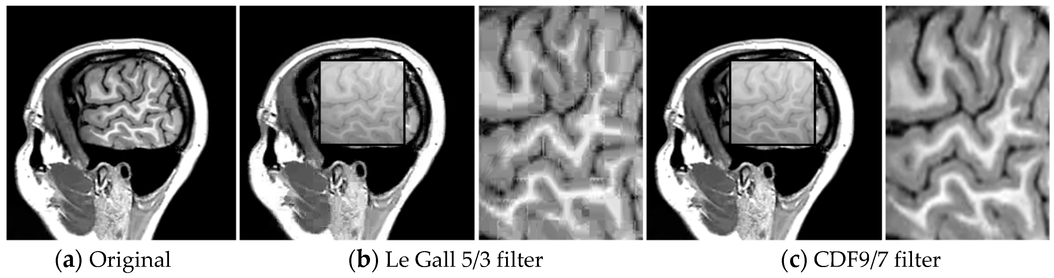
In this experiment, MRI video is encoded using the Bandelet-SPIHT algorithm for various bit rates. In order to find the most suitable wavelet filter for different test images based upon objective quality measures for video compression, biorthogonal family was considered. Thus, biorthogonal wavelets CDF (Cohen–Daubechies–Feauveau) 9/7 (nine coefficients in decomposition low-pass and seven in decomposition highpass filters) and Le Gall 5/3 (five coefficients in decomposition low-pass and three in decomposition high-pass filters) are selected.
The choice of these filters is justified by their simplicity, symmetry and their compact support (localization in space).
By a subjective quality assessment of images shown in
Figure 8, we opt for CDF 9/7, which reduces the level of artifacts. Indeed, the obtained results show that the recovered frame using the bandelet algorithm + SPIHT is close to the original frame.
It is worth noting the presence of blurred areas in the image when Le Gall 5/3 filters are used.
Objective measurement of video quality (PSNR, SSIM and VIF) between (bandelet + SPIHT) algorithm and (wavelet + SPIHT) applied to coronary angiography test frame at various bit rates are illustrated in
Figure 9.
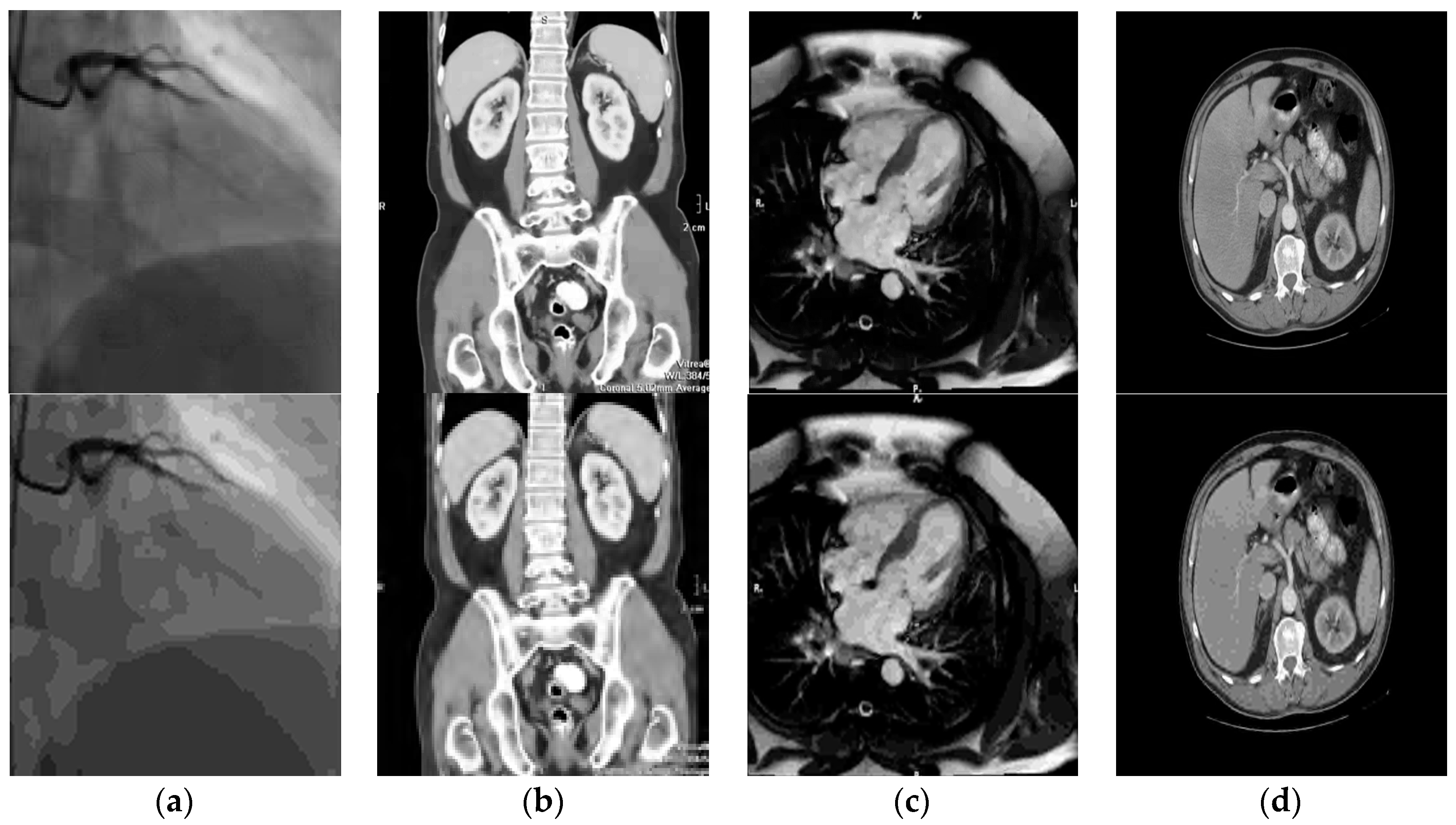
Figure 10 is an illustration of a sample of medical images from our large databases used for benchmarking (subjective quality assessment by visual inspection).
The images shown in
Figure 10 are a simple illustration and their technical and medical characteristics are summarized in
Table 1 (see also
Figure 6). They represent: (
a) Coronary angiography-X-ray; (
b) abdomen/pelvis-computed tomography (CT); (
c) heart-axial MRI; (
d) bladder-MRI.
- 1
The performance of bandelet-SPIHT algorithm is superior to that of SPIHT (wavelet-based).
- 2
Bandelet-SPIHT is able to capture complex geometric contents of images and surfaces and reduce drastically existing redundancy in video while classical SPIHT (based on discrete wavelet transform) is subject to artifacts.
- 3
The bandelet-SPIHT algorithm gives better results in the case of CDF 9/7 wavelet filters than in the case of Le Gall 5/3.
4.4. Bandelet-SPIHT Versus Standard Encoders Comparison
Advanced video coding (AVC), also known as H.264/MPEG-4, and its successor high-efficiency video coding (HEVC), also known as H.265 and MPEG-H Part 2, are compared to the proposed coder bandelet-SPIHT using data metrics, namely PSNR (dB).
Figure 11 shows the performance, in terms of PSNR vs bitrate, of three compression techniques H264/AVC, H265/HEVC and bandelet-SPIHT. Each value represents an average within its confidence interval. For example, for 270 kbps, the PSNR obtained by bandelet-SPIHT is higher than that produced by the other methods and its confidence interval is tightened around the mean value. On the other hand, for 2260 kbps, the PSNR obtained by bandelet-SPIHT is lower than that produced by HEVC. In addition, its confidence interval is asymmetric with a greater tendency towards lower values. Consequently, we will have little confidence in this average value obtained by the algorithm proposed for high data rates.
As illustrated in
Figure 11, the proposed method demonstrates a relatively better performance compared to the standard video coding AVC and HEVC in terms of PSNR. For example, for a bit rate greater than 1.3 Mbps, it is clear that in terms of PSNR, the performance of the proposed algorithm (bandelet-SPIHT) is lower than that of HEVC but almost always higher than that of AVC. And for low bit rates, our encoder outperforms video coding standards. For example, for 0.6 Mbps, our method exceeds AVC and HEVC by 3 dB and 0.5 dB respectively.
And for low bit rates, our encoder outperforms video coding standards. For example, for 0.6 Mbps, our method exceeds AVC and HEVC by 3 dB and 0.5 dB respectively.
It is well-known that complex images, fast camera movements and action scenes require high bitrate. In this context, HEVC is the most efficient technology to date.
Those with fixed scenes, which are easier to encode, require a slower rate, as is the case in medical imaging. In this context, bandelet-SPIHT is superior at low bitrates due to its ability to capture the geometric complexity of the image structure and its multi-resolution analysis.
For the tests, we used an improved version of HEVC sometimes called HEVC screen content coding extension. This standardization effort was developed to leverage the unique characteristics of computer-generated and digitally-captured videos. The intra block copy mode takes advantage of the presence of exact copies of blocks between different pictures in a video sequence.
The test conditions include video sequences comprising a variety of resolutions and content types (text and graphics with motion, camera-captured content, mixed content and animation). For each sequence, two color formats are tested. One is in RGB and the other is in Y CB CR (Y is the luma component and CB and CR are the blue-difference and red-difference chroma components) and several of the 4:2:0 sequences are generated from their 4:4:4 correspondences.
Three test configurations, i.e., all intra (AI), random access (RA) and low-delay B (LB) were used. For lossy coding, four QPs (quantization parameters), {22, 27, 32, 37}, were applied.
The statistical study we have carried out is in line with the recommendations of ITU—Telecommunications Standardization Sector, and more specifically the Video Coding Experts Group.
Indeed, the benchmarking used to measure performance of HEVC and the proposed codec was made partly by experts in video via quality criteria adapted to the human visual system such as SSIM and VIF (objective quality metrics) and partly by clinicians or PhD students (subjective quality assessment) from our medical research institute (INSERM). However, the subjective improvement measured somewhat exceeds the improvement measured by the PSNR metric.
4.5. Computational Complexity
We cannot directly compare the temporal performance of the proposed algorithm with that of H264/AVC and H265/HEVC, due to their structural difference and their compression concept based on totally different philosophies. However, we will develop and clarify this issue, which is crucial to understanding the purpose of our work.
We will focus on two fundamental differences between the MPEG4 family (AVC and HEVC) and bandelet-SPIHT:
Unlike MPEG4’s (H264/AVC and H265/HEVC) use of both intra- and inter-frame encoding, bandelet-SPIHT employs only intra-frame encoding. This means that each frame is compressed individually, and no attention is paid by the encoder to either previous or following frames, and so it is not predictive in any way.
Consequently, for bandelet-SPIHT the (time) latency to compress a frame is shorter (as the codec does not have to rely on generating forward and reverse differences between frames).
The type of transform used by AVC and HEVC is DCT while our compression algorithm uses 2nd-generation wavelets (bandelet transform).
For an image of pixels, the computational complexity of the best bandelet basis algorithm is whereas for the DCT the computational complexity can be approximated by . This shows that the calculation of bandelet transform is more complex than that of the DCT
From these two considerations, we can conclude that the computation time required for H264/AVC compression is comparable to that of bandelet-SPIHT, which has been confirmed experimentally.
For high spatial resolution videos, the increase of computational complexity for HEVC is about 25% on the average compared to AVC (and thus for bandelet-SPIHT), which seems quite reasonable with considerations of significant coding efficiency improvements.
Therefore, we can conclude that the computational complexity between bandelet-SPIHT and H264/AVC is of the same order, whereas that of HEVC is significantly higher. However, H.265/HEVC technology has the capability of doubling the compression efficiency of H.264/AVC. What this means is that H.265 uses only half the bitrate otherwise used by H.264/AVC when transmitting images [
9,
10]. So, H.265/HEVC significantly reduces the storage and bandwidth requirements during video encoding, which is highly beneficial for both software and hardware usage.
5. Conclusions
The objective motivating our study was to propose a coding method with high performances in terms of visual quality and PSNR at low bit rates. The bandelets using a SPIHT encoder is an effective condidate meeting the specific requirements of our application in the medical field and particulary in medical imaging where the quality of the image at low bit rates is a major requirement for the practitioner.
In order to show the efficiency of bandelet-SPIHT algorithm, a set of medical sequences as test examples is considered. At low bit rates, the bandelet-SPIHT algorithm gives significantly better results (PSNR metric) comparing to some cutting-edge coding techniques such as H.26x family (namely H.264 and H.265). In addition, the computational complexity of the proposed algorithm is of the same order of magnitude as that of H264/AVC but significantly lower than that of H265/HEVC.
From this point of view, the expected goal is achieved and the prospects for application in medical imaging are promising.
Geometric image compression methods are a very dynamic search direction. One could mention the construction of transformations that adapt automatically to the geometry without the need to specify it. A consensus is growing in the scientific community that geometry is the key to significantly improve current compression methods. However, HEVC compressed videos may incur severe quality degradation, particularly at low bit-rates. Thus, it is necessary to enhance the visual quality of HEVC videos at the decoder side.
It is in this area that improvements are expected and research is ongoing [
34]. Another useful way is to improve objective metrics [
35] to evaluate the quality of videos automatically.


 ,
, 


