A Task Parameter Inference Framework for Real-Time Embedded Systems

Abstract

While recent studies addressed security attacks in real-time embedded systems, most of them assumed prior knowledge of parameters of periodic tasks, which is not realistic under many environments. In this paper, we address how to infer task parameters, from restricted information obtained by simple system monitoring. To this end, we first develop static properties that are independent of inference results and therefore applied only once in the beginning. We further develop dynamic properties each of which can tighten inference results by feeding an update of the inference results obtained by other properties. Our simulation results demonstrate that the proposed inference framework infers task parameters for RM (Rate Monotonic) with reasonable tightness; the ratio of exactly inferred task periods is 95.3% and 65.6%, respectively with low and high task set use. The results also discover that the inference performance varies with the monitoring interval length and the task set use.

1. Introduction

Real-Time Embedded Systems (RTES) have been deployed in time-critical environments, often involving control tasks each of which invokes a series of jobs with periodic releases, which has been widely studied in the industrial informatics community [1,2,3,4,5,6]. While traditional RTES have been little exposed to security attacks due to isolation from the external world and use of specialized hardware/protocol, increased connectivity yields new security attacks on RTES. Therefore, recent studies have addressed vulnerability issues by incorporating security mechanisms into RTES, without compromising timing constraints [7,8,9]; for example, a study in [8] has proposed a schedule randomization protocol against timing inference attacks such as side-channel or covert-channel attacks [10,11,12,13,14,15]. Also, targeting Electronic Control Units (ECU), some studies have developed a new denial-of-service attack [16] and a new intrusion detection system [17].

The attacks presented by those existing studies (from both defensive and offensive aspects) assume that the adversary knows important information of task parameters such as task period and actual/worst-case execution time; for example, the attacks in [8,9] and those in [16,17] assume knowledge of all task parameters and some task parameters including task priority ordering, respectively. Since information of task parameters is not necessarily open to the public, we need (i) to know whether it is feasible to infer task parameters from restricted information obtained by simple system monitoring and (ii) to develop a systematic way how to infer, both of which have not been fully addressed in existing studies. As shown in Figure 1, it is very challenging to infer task parameters, from information of the task index of currently-executing jobs (Section 2 will discuss how to obtain the information by simple system monitoring).

In this paper, we propose a framework to infer task parameters, only from information about the task index of currently-executing jobs, and we apply the framework to RM (Rate Monotonic) [18]; once developed, the framework makes it possible to predict future job release and execution patterns of a given RTES so as to facilitate security attacks. To this end, we develop two types of properties that can narrow down (a) the feasible range of each task period and (b) the feasible group of each task’s execution chunks that belong to the same job. First, we design static properties that are independent of inference results, which are therefore applied only once in the beginning. Second, we propose dynamic properties, each of which can yield tighter inference for (a) and (b) by feeding an update of the inference results obtained by other properties. Since all the properties to be developed in this paper do not assume any prior knowledge of job release times, task/job priority ordering, and distribution of actual execution times (many studies for security issues in RTES implicitly assume that the actual execution time is static [8,9,11,19]), the proposed framework successfully operates with various environments.

Our simulation results for the proposed inference framework make the following implications. First, the proposed framework infers task parameters for RM with reasonable tightness; the ratio of exactly inferred task periods is 95.3% and 65.6%, respectively with low and high task set use. Second, the inference performance gets improved, as the system use decreases or the monitoring interval length increases.

In summary, this paper makes the following contributions:

• Introduction of a task parameter inference problem for given restricted information,
• Development of useful properties that narrow down (a) and (b),
• Demonstration of reasonably tight inference of task parameters for RM, and
• Identification of factors that affect inference performance: the monitoring interval length and the system use.

The remainder of this paper is structured as follows. Section 2 explains the system and adversary model. Section 3 presents the overall structure of the inference framework. Section 4 and Section 5 propose static and dynamic properties, respectively. Section 6 evaluates the effectiveness of the proposed framework, and finally, Section 9 concludes the paper.

2. System and Adversary Model

System model. We target a real-time embedded system which deploys a uniprocessor, and the system has a set of periodic real-time tasks. Each task ${\tau }_i\in \tau$ is modeled by the period ($T_i$) and the worst-case execution time ($C_i$); ${\tau }_i$ invokes a series of jobs, each separated from its predecessor by exactly $T_i$ time units (in this paper, we assume quantum-based time; without loss of generality, let one time unit be the quantum length, and therefore all task/job parameters are non-zero natural numbers). We do not assume any relationship between jobs belonging to different tasks; therefore, individual tasks do not necessarily invoke their jobs in a synchronous manner. Different from recent studies for security issues in real-time systems [8,9,11], the actual execution time of each job of ${\tau }_i$ (denoted by $A_i\left(J\right)$ for job J) is not necessarily equal to $C_i$; instead, $1\le A_i\left(J\right)\le C_i$ holds.

We target one of the most popular preemptive real-time scheduling algorithms: RM, which gives a higher priority to a job whose invoking task’s period is shorter. Each task has a unique task index, but it does not necessarily imply the task priority. We assume that the target system normally operates without any deadline miss for all jobs.

Adversary model. The main objective of the adversary is to infer task parameters $C_i$ and $T_i$ for every task ${\tau }_i\in \tau$, which potentially yields various security attacks such as side-channel attacks [10,11,12,13] or covert-channel attacks [15]. We consider that the adversary monitors the target system during the monitoring interval (denoted by $\mathrm{MI}$) and obtains very restricted information—the task index of currently-executing jobs, which is feasible for many environments such as ECU connected with control area network [16,17]. Please note that the task index information does not necessarily imply that we should know the task indexes used in the system; instead, we only need to distinguish every task from other tasks, which is feasible using various techniques such as [20]. For example, an attacker can number tasks in Figure 1 after s/he differentiates all tasks.

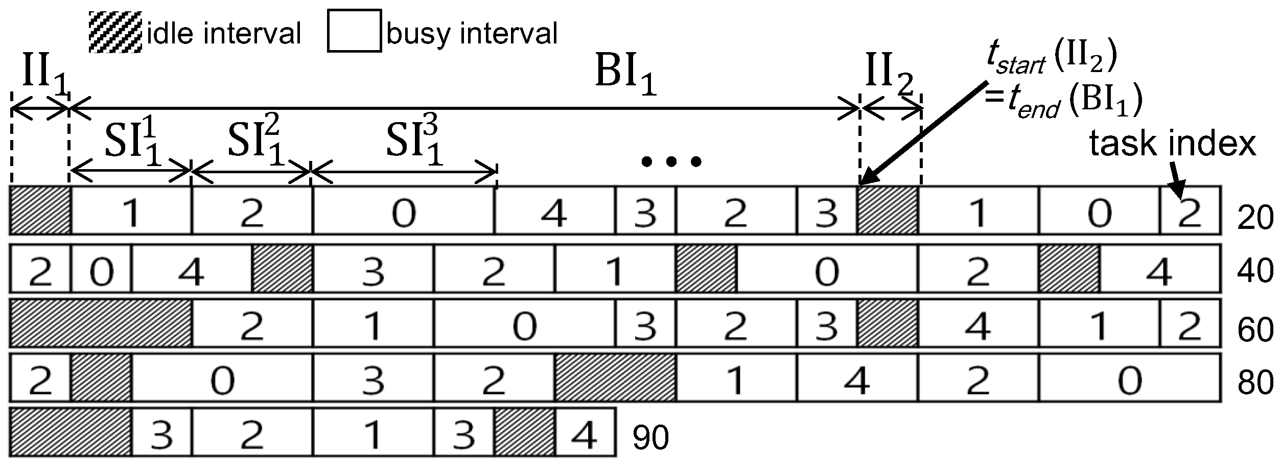
Notations. We can formally express the monitoring interval ($\mathrm{MI}$) as follows. From knowledge of the task index of currently-executing jobs, we naturally track which task was executed and whether CPU was idle or busy in each time quantum. We define the busy (likewise idle) interval as an interval in which a series of jobs are consecutively executed without idling CPU (likewise no job is executed). We can express $\mathrm{MI}$ as a union of busy and idle intervals in which different types of intervals alternate (for the ease of presentation, we assume that $\mathrm{MI}$ starts with an idle interval), meaning that $\mathrm{MI}={\mathrm{II}}_1\cup {\mathrm{BI}}_1\cup {\mathrm{II}}_2\cup {\mathrm{BI}}_2\cup \dots$, where ${\mathrm{BI}}_x$ (likewise ${\mathrm{II}}_x$) denote the xth busy (likewise idle) interval, as shown in Figure 1. We also define a subinterval as an interval between the time instant when a job of a task starts or resumes its execution and that when it stops its execution by the scheduler; therefore, each job in its subinterval continuously runs without being interrupted by any other job or idle interval. Let ${\mathrm{SI}}_x^a$ denote the ath subinterval in ${\mathrm{BI}}_x$. By definition, a full or partial execution of a single job is performed in each subinterval, and it is not allowed to execute more than one job in each subinterval. As $\mathrm{MI}$ is decomposed into ${\mathrm{II}}_x$ and ${\mathrm{BI}}_x$, ${\mathrm{BI}}_x$ can be decomposed into ${\mathrm{SI}}_x^1\cup {\mathrm{SI}}_x^2\cup \dots$, as shown in Figure 1.

In this paper, let $N_{\mathrm{BI}}$ denote the number of busy intervals in $\mathrm{MI}$, and $N_{{\mathrm{SI}}_x}$ denote the number of subintervals in ${\mathrm{BI}}_x$. Also, let $\tau \left({\mathrm{SI}}_x^a\right)$ denote the task executed in ${\mathrm{SI}}_x^a$. Finally, let $t_{\mathrm{start}}\left(\mathrm{Interval}\right)$ and $t_{\mathrm{end}}\left(\mathrm{Interval}\right)$ denote the start and end time of $\mathrm{Interval}$; for example, $t_{\mathrm{start}}\left(\mathrm{MI}\right)$, $t_{\mathrm{start}}\left({\mathrm{BI}}_x\right)$, and $t_{\mathrm{start}}\left({\mathrm{SI}}_x^a\right)$ denote the start time of $\mathrm{MI}$, ${\mathrm{BI}}_x$, and ${\mathrm{SI}}_x^a$, respectively.

3. Inference Framework Overview

The proposed framework aims at inferring task parameters $(T_i,C_i)$ for every task executed in the monitoring interval $\mathrm{MI}$, so as to facilitate other security attacks. Once we investigate $\mathrm{MI}$, we can arrange the following information:

${\mathrm{Info}}_1$.

A set of tasks executed in $\mathrm{MI}$ (denoted by $\tau$), and

${\mathrm{Info}}_2$.

$t_{\mathrm{start}}\left({\mathrm{BI}}_x\right)$ and $t_{\mathrm{end}}\left({\mathrm{BI}}_x\right)$ for every $1\le x\le N_{\mathrm{BI}}$, and $t_{\mathrm{start}}\left({\mathrm{SI}}_x^a\right)$, $t_{\mathrm{end}}\left({\mathrm{SI}}_x^a\right)$ and $\tau \left({\mathrm{SI}}_x^a\right)$ for every pair of $1\le x\le N_{\mathrm{BI}}$ and $1\le a\le N_{{\mathrm{SI}}_x}$.

Based on ${\mathrm{Info}}_1$ and ${\mathrm{Info}}_2$, the framework develops properties regarding task periods and subinterval groups for job separation. While it is straightforward to require the former, the need/role of the latter will be explained now. The hth subinterval group of ${\tau }_k$ (denoted by ${\mathrm{SG}}_h\left({\tau }_k\right)$) is defined as a group of subintervals in each of which the potentially same job of ${\tau }_k$ is executed. What we meant by “the potentially same job” is as follows. If two subintervals ${\mathrm{SI}}_x^a$ and ${\mathrm{SI}}_y^b$ satisfying $\tau \left({\mathrm{SI}}_x^a\right)=\tau \left({\mathrm{SI}}_y^b\right)={\tau }_k$ belong to different subinterval groups, then it means that a job of ${\tau }_k$ executed in ${\mathrm{SI}}_x^a$ is different from that in ${\mathrm{SI}}_y^b$. Otherwise, a job of ${\tau }_k$ executed in ${\mathrm{SI}}_x^a$ can be either different from or the same as that in ${\mathrm{SI}}_y^b$. Whenever we find new evidence that different jobs of a task are executed in subintervals belonging to the same subinterval group, we split the subinterval group into two.

Once we gather sufficiently specific information of subinterval groups and then combine it to task period information, we finally know not only $T_i$, but also statistics for $A_i\left(J\right)$, allowing the prediction of $C_i$. To this end, we maintain the following information regarding task periods and subinterval groups:

${\mathrm{Info}}_3$.

$T_i^{-}$ and $T_i^{+}$ for every ${\tau }_i\in \tau$, and

${\mathrm{Info}}_4$.

Subintervals in ${\mathrm{SG}}_h\left({\tau }_k\right)$, $t_{\mathrm{release}}^{-}\left(J^{\mathrm{earliest}}\left({\mathrm{SG}}_h\left({\tau }_k\right)\right)\right)$,

$t_{\mathrm{release}}^{+}\left(J^{\mathrm{earliest}}\left({\mathrm{SG}}_h\left({\tau }_k\right)\right)\right)$, $t_{\mathrm{release}}^{-}\left(J^{\mathrm{latest}}\left({\mathrm{SG}}_h\left({\tau }_k\right)\right)\right)$, and

$t_{\mathrm{release}}^{+}\left(J^{\mathrm{latest}}\left({\mathrm{SG}}_h\left({\tau }_k\right)\right)\right)$ for every pair of ${\tau }_k\in \tau$ and possible h,

Here, $T_i^{-}$ and $T_i^{+}$ denote the lower and upper bounds of $T_i$, respectively. $t_{\mathrm{release}}\left(J\right)$, $t_{\mathrm{release}}^{-}\left(J\right)$, and $t_{\mathrm{release}}^{+}\left(J\right)$ also denote the release time of a job J, its lower bound, and its upper bound. $J^{\mathrm{earliest}}\left({\mathrm{SG}}_h\left({\tau }_k\right)\right)$ and $J^{\mathrm{latest}}\left({\mathrm{SG}}_h\left({\tau }_k\right)\right)$ denote a job with the earliest and latest release time among jobs executed in subintervals in ${\mathrm{SG}}_h\left({\tau }_k\right)$. Therefore, ${\mathrm{Info}}_4$ includes information regarding the feasible range of release times of jobs with the earliest and latest release times, and will be used for deriving ${\mathrm{Info}}_3$ in the later sections.

Then, the proposed inference framework’s objective can be expressed by obtaining ${\mathrm{Info}}_3$ and ${\mathrm{Info}}_4$ as tightly as possible, and the framework operates with the following steps.

${\mathrm{Step}}_1$.

Obtain ${\mathrm{Info}}_1$ and ${\mathrm{Info}}_2$ from $\mathrm{MI}$.

${\mathrm{Step}}_2$.

Set the default values to ${\mathrm{Info}}_3$ and ${\mathrm{Info}}_4$.

${\mathrm{Step}}_3$.

Apply static properties for ${\mathrm{Info}}_3$ and ${\mathrm{Info}}_4$.

${\mathrm{Step}}_4$.

Apply dynamic properties for ${\mathrm{Info}}_3$ and ${\mathrm{Info}}_4$.

${\mathrm{Step}}_5$.

If there is any change of ${\mathrm{Info}}_3$ and ${\mathrm{Info}}_4$ in ${\mathrm{Step}}_4$, go to ${\mathrm{Step}}_4$; otherwise, stop the inference framework.

In ${\mathrm{Step}}_2$, we set $T_i^{-}$ and $T_i^{+}$ to 1 and ${\mathrm{MAX}}_T$ (sufficiently large value) for every ${\tau }_i\in \tau$, respectively. Also, we assign only one unified subinterval group ${\mathrm{SG}}_{\mathrm{uni}}\left({\tau }_k\right)$ for every ${\tau }_k\in \tau$, and set $t_{\mathrm{release}}^{-}(J^{\mathrm{earliest}}\left({\mathrm{SG}}_h\left({\tau }_k\right)\right)$ and $t_{\mathrm{release}}^{-}(J^{\mathrm{latest}}\left({\mathrm{SG}}_h\left({\tau }_k\right)\right)$ to $t_{\mathrm{start}}\left(\mathrm{MI}\right)$, and $t_{\mathrm{release}}^{+}(J^{\mathrm{earliest}}\left({\mathrm{SG}}_h\left({\tau }_k\right)\right)$ and $t_{\mathrm{release}}^{+}(J^{\mathrm{latest}}\left({\mathrm{SG}}_h\left({\tau }_k\right)\right)$ to $t_{\mathrm{end}}\left(\mathrm{MI}\right)$; the unified subinterval group will be split by properties to be presented in later sections.

When it comes to ${\mathrm{Step}}_3$, static properties to be developed in Section 4, rely on ${\mathrm{Info}}_1$ and ${\mathrm{Info}}_2$ only. Hence, the properties are not affected by any change of ${\mathrm{Info}}_3$ and ${\mathrm{Info}}_4$, implying that we apply the properties only once in the beginning.

In ${\mathrm{Step}}_4$, dynamic properties to be developed in Section 5, utilize some of ${\mathrm{Info}}_3$ and ${\mathrm{Info}}_4$, and have potential to further narrow down ${\mathrm{Info}}_3$ and ${\mathrm{Info}}_4$, from an update of ${\mathrm{Info}}_3$ and ${\mathrm{Info}}_4$ by other properties. Therefore, we repeatedly apply the properties whenever there is an update of ${\mathrm{Info}}_3$ and ${\mathrm{Info}}_4$.

Once we apply our inference framework with ${\mathrm{Step}}_1$ to ${\mathrm{Step}}_5$, we are able to not only infer each task period, but also differentiate different jobs belonging to the same task, which implies that we know the execution time of each job. Therefore, for the remainder of the paper, we focus on inferring each task period.

4. Task Inference by Static Properties

In this section, we aim at inferring ${\mathrm{Info}}_3$ and ${\mathrm{Info}}_4$, and derive static properties that are independent of ${\mathrm{Info}}_3$ and ${\mathrm{Info}}_4$.

The first static property determines the range of the release times of the earliest and latest jobs in a subinterval group as follows.

Subinterval Group Property 1. 

We can split the unified subinterval group ${\mathit{SG}}_{\mathit{uni}}\left({\tau }_k\right)$ into several groups each of which includes subintervals belonging to the same busy interval. After splitting, the following inequalities hold for a subinterval group ${\mathit{SG}}_h\left({\tau }_k\right)$ which includes subintervals ${\mathit{SI}}_x^{b_1},{\mathit{SI}}_x^{b_2},\dots ,{\mathit{SI}}_x^{b_m}$ where $b_1<b_2<\dots <b_m$.

$$\begin{array}{c}\hfill t_{\mathit{start}}\left({\mathit{BI}}_x\right)\le t_{\mathit{release}}\left(J^{\mathit{earliest}}\left({\mathit{SG}}_h\left({\tau }_k\right)\right)\right)\le t_{\mathit{start}}\left({\mathit{SI}}_x^{b_1}\right),\end{array}$$

(1)

$$\begin{array}{c}\hfill t_{\mathit{start}}\left({\mathit{BI}}_x\right)\le t_{\mathit{release}}\left(J^{\mathit{latest}}\left({\mathit{SG}}_h\left({\tau }_k\right)\right)\right)\le t_{\mathit{start}}\left({\mathit{SI}}_x^{b_m}\right).\end{array}$$

(2)

In short, the release time of a job with the earliest release time among jobs executed in subintervals in ${\mathit{SG}}_h\left({\tau }_k\right)$ is between the start time of the busy interval and the start time of the earliest subinterval in ${\mathit{SG}}_h\left({\tau }_k\right)$. Also, the release time of a job with the latest release time among jobs executed in subintervals in ${\mathit{SG}}_h\left({\tau }_k\right)$ is between the start time of the busy interval and the start time of the latest subinterval in ${\mathit{SG}}_h\left({\tau }_k\right)$.

In addition, if $b_1=1$ (i.e., ${\mathit{SI}}_x^{b_1}$ is the earliest subinterval in its busy interval ${\mathit{BI}}_x$), then we can find an exact value of the release time of the earliest job in ${\mathit{SG}}_h\left({\tau }_k\right)$ as follows:

$$\begin{array}{c}\hfill t_{\mathit{release}}\left(J^{\mathit{earliest}}\left({\mathit{SG}}_h\left({\tau }_k\right)\right)\right)=t_{\mathit{start}}\left({\mathit{BI}}_x\right).\end{array}$$

(3)

Proof. 

Since no job is released and executed in an idle interval, the release time of any job in a busy interval cannot be earlier than the starting time of the busy interval, implying the first inequalities in Equations (1) and (2). The second inequalities in Equations (1) and (2) hold as follows. Since there exists a job which starts its execution at $t_{\mathrm{start}}\left({\mathrm{SI}}_x^{b_1}\right)$, a job with the earliest release time in ${\mathrm{SG}}_h\left({\tau }_k\right)$ cannot be released later than $t_{\mathrm{start}}\left({\mathrm{SI}}_x^{b_1}\right)$. Similarly, since the latest subinterval in which ${\tau }_k$ is executed starts at $t_{\mathrm{start}}\left({\mathrm{SI}}_x^{b_m}\right)$, a job with the latest release time in ${\mathrm{SG}}_h\left({\tau }_k\right)$ cannot be released later than $t_{\mathrm{start}}\left({\mathrm{SI}}_x^{b_m}\right)$. Equation (3) immediately holds because no job is released and executed in an idle interval. □

Now, we present useful properties that narrow down the range of every task period, starting from the property indicating the period of a task is at least as much as the length of a subinterval in which the task is executed.

Task Period Property 1. 

The following inequality holds for ${\mathit{SI}}_x^a$ satisfying $\tau \left({\mathit{SI}}_x^a\right)={\tau }_k$, for every pair of $1\le x\le N_{\mathit{BI}}$ and $1\le a\le N_{{\mathit{SI}}_x}$:

$$\begin{array}{c}\hfill T_k\ge t_{\mathit{end}}\left({\mathit{SI}}_x^a\right)-t_{\mathit{start}}\left({\mathit{SI}}_x^a\right).\end{array}$$

(4)

The inequality means that the period of ${\tau }_k$ is at least the difference between the start and end time of each subinterval for ${\tau }_k$.

Proof. 

The length of ${\mathrm{SI}}_x^a$ is no longer than $A_k\left(J\right)$ for every job J of ${\tau }_k$, and $A_k\left(J\right)\le C_k\le T_k$ holds. Therefore, the property holds. □

Based on the observation that any job cannot be released within an idle interval, we derive the following property.

Task Period Property 2. 

The following inequality holds for ${\mathit{BI}}_x$ for every $1\le x\le N_{\mathit{BI}}-1$:

$$\begin{array}{c}\hfill T_k>\frac{t_{\mathit{start}}\left({\mathit{BI}}_{x+1}\right)-t_{\mathit{end}}\left({\mathit{BI}}_x\right)}{2}.\end{array}$$

(5)

The inequality means that the period of ${\tau }_k$ is at least half of the difference between the start time of the next busy interval and the end time of the current busy interval.

Proof. 

Suppose that Equation (5) is wrong. Then, there exists at least one job released in $[t_{\mathrm{end}}\left({\mathrm{BI}}_x\right),t_{\mathrm{end}}\left({\mathrm{BI}}_x\right)+\frac{t_{\mathrm{start}}\left({\mathrm{BI}}_{x+1}\right)-t_{\mathrm{end}}\left({\mathrm{BI}}_x\right)}{2}]$, and the job’s deadline is no later than $t_{\mathrm{start}}\left({\mathrm{BI}}_{x+1}\right)$, meaning that the idle interval $[t_{\mathrm{end}}\left({\mathrm{BI}}_x\right),t_{\mathrm{start}}\left({\mathrm{BI}}_{x+1}\right))$ subsumes the interval between the job’s release and deadline, which implies no execution of the job. This contradicts the supposition. □

Analyzing the job release/execution patterns, we can derive the following property regarding each task period.

Task Period Property 3. 

Suppose that there are at most $n-2$ subintervals satisfying $\tau \left({\mathit{SI}}_x^a\right)={\tau }_k$ within a continuous interval of length $n·L$, where n is a natural number not smaller than 2. Then, the following inequality holds:

$$\begin{array}{c}\hfill T_k>L.\end{array}$$

(6)

Proof. 

Suppose that Equation (6) is wrong; we will show the contradiction. If we focus on an interval of length $n·L$, the interval contains at least $n-1$ jobs whose release times and deadlines are within the interval. Since each job has at least one unit of execution, there should be at least $n-1$ subintervals. This contradicts the supposition. □

Please note that we can apply a binary search to find the largest L in Task Period Property 3. This is because if we find a continuous interval of length $n·L$ satisfying the property, we also find that of length $n·L^{\prime }$ (if $L^{\prime }<L$).

We also note that it may be time-consuming to test all feasible intervals of given length $n·L$ within $\mathrm{MI}$. To alleviate computation cost, we may select some of candidate intervals, e.g., $[t_{\mathrm{start}}\left(\mathrm{MI}\right),t_{\mathrm{start}}\left(\mathrm{MI}\right)+n·L)$, $[t_{\mathrm{start}}\left(\mathrm{MI}\right)+n·L,t_{\mathrm{start}}\left(\mathrm{MI}\right)+2·n·L)$, $[t_{\mathrm{start}}\left(\mathrm{MI}\right)+2·n·L,t_{\mathrm{start}}\left(\mathrm{MI}\right)+3·n·L)$ and so on. Likewise, we may also limit the number of trials for n.

Example 1.

We explain how static properties work using an example in Figure 1. In the example, the monitoring interval $\mathit{MI}$ is $[0,90)$, and there are 5 tasks: ${\tau }_0$, ${\tau }_1$, ${\tau }_2$, ${\tau }_3$ and ${\tau }_4$. Due to the space limit, we explain how the framework narrows down the range of $T_2$ of ${\tau }_2$. After applying Task Period Property 1, we know $T_2\ge 2$. Since the length of the longest idle interval is 3, Task Period Property 2 also yields $T_2>1.5$. If we focus on $[13,19)$, there is no execution of ${\tau }_2$, deriving $T_2>3$ from Task Period Property 3. Considering the quantum length equal to 1, we conclude $T_2\ge 4$. The feasible range of $T_i$ for all tasks are shown in

Table 1. The feasible range of each task period after applying static properties.

Task Index	0	1	2	3	4
$T_i^{-}$	12	11	4	11	13
$T_i^{+}$	${\mathrm{MAX}}_T$	${\mathrm{MAX}}_T$	${\mathrm{MAX}}_T$	${\mathrm{MAX}}_T$	${\mathrm{MAX}}_T$

.

5. Task Inference by Dynamic Properties

Different from static properties, dynamic properties utilize ${\mathrm{Info}}_3$ and ${\mathrm{Info}}_4$; we can feed an update of ${\mathrm{Info}}_3$ and ${\mathrm{Info}}_4$ by a dynamic property back to other dynamic properties, potentially improving inference performance by collaboration of different dynamic properties.

We first narrow down the range of the release time of the earliest and latest jobs in a subinterval group as follows.

Subinterval Group Property 2. 

Suppose that there are two consecutive subinterval groups of ${\tau }_k$: (i) ${\mathit{SG}}_{h-1}\left({\tau }_k\right)$ consisting of subintervals ${\mathit{SI}}_x^{a_1},{\mathit{SI}}_x^{a_2},\dots ,{\mathit{SI}}_x^{a_n}$ where $a_1<a_2<\dots <a_n$, and (ii) ${\mathit{SG}}_h\left({\tau }_k\right)$ consisting of subintervals ${\mathit{SI}}_y^{b_1},{\mathit{SI}}_y^{b_2},\dots ,{\mathit{SI}}_y^{b_m}$ where $b_1<b_2<\dots <b_m$, and $x\le y$. Then, we can determine the range of the release times of the earliest and latest jobs in ${\mathit{SG}}_h\left({\tau }_k\right)$ as follows (here, the term “two consecutive subinterval groups” ${\mathit{SG}}_{h-1}\left({\tau }_k\right)$ and ${\mathit{SG}}_h\left({\tau }_k\right)$ implies that there is no subinterval group which is later than ${\mathit{SG}}_{h-1}\left({\tau }_k\right)$ and earlier than ${\mathit{SG}}_h\left({\tau }_k\right)$).

$$\begin{array}{c}\hfill t_{\mathit{end}}\left({\mathit{SI}}_x^{a_n}\right)\le t_{\mathit{release}}\left(J^{\mathit{earliest}}\left({\mathit{SG}}_h\left({\tau }_k\right)\right)\right)\le t_{\mathit{start}}\left({\mathit{SI}}_y^{b_1}\right),\end{array}$$

(7)

$$\begin{array}{c}\hfill t_{\mathit{end}}\left({\mathit{SI}}_x^{a_n}\right)\le t_{\mathit{release}}\left(J^{\mathit{latest}}\left({\mathit{SG}}_h\left({\tau }_k\right)\right)\right)\le t_{\mathit{start}}\left({\mathit{SI}}_y^{b_m}\right).\end{array}$$

(8)

The structure of the above inequalities are similar to that of Subinterval Group Property 1.

Proof. 

Suppose that $t_{\mathrm{release}}\left(J^{\mathrm{earliest}}\left({\mathrm{SG}}_h\left({\tau }_k\right)\right)\right)$ is earlier than $t_{\mathrm{end}}\left({\mathrm{SI}}_x^{a_n}\right)$. Then, it contradicts the definition of a subinterval group—different jobs should be executed in subintervals in different groups. Therefore, the first inequalities in Equations (7) and (8) hold. We already prove the second inequalities in Equations (7) and (8) in Subinterval Group Property 1. □

Subinterval Group Property 2 is effective for the situation where all subintervals in two consecutive subinterval groups belong to the same busy interval. Whenever a subinterval is split by some properties to be presented later, the property yields a tighter value of $t_{\mathrm{release}}^{-}\left(J^{\mathrm{earliest}}\left({\mathrm{SG}}_h\left({\tau }_k\right)\right)\right)$ and $t_{\mathrm{release}}^{-}\left(J^{\mathrm{latest}}\left({\mathrm{SG}}_h\left({\tau }_k\right)\right)\right)$ than Subinterval Group Property 1. This is because, $t_{\mathrm{end}}\left({\mathrm{SI}}_x^{a_n}\right)$ in Equations (7) and (8) is no earlier than $t_{\mathrm{start}}\left({\mathrm{BI}}_x\right)$ in Equations (1) and (2), if ${\mathrm{SG}}_{h-1}\left({\tau }_k\right)$ and ${\mathrm{SG}}_h\left({\tau }_k\right)$ belong to the same busy interval.

Using the above subinterval group property, we can determine the range of each task period as follows.

Task Period Property 4. 

Suppose that there are two consecutive subinterval groups of ${\tau }_k$: (i) ${\mathit{SG}}_{h-1}\left({\tau }_k\right)$ consisting of subintervals ${\mathit{SI}}_x^{a_1},{\mathit{SI}}_x^{a_2},\dots ,{\mathit{SI}}_x^{a_n}$ where $a_1<a_2<\dots <a_n$, and (ii) ${\mathit{SG}}_h\left({\tau }_k\right)$ consisting of subintervals ${\mathit{SI}}_y^{b_1},{\mathit{SI}}_y^{b_2},\dots ,{\mathit{SI}}_y^{b_m}$ where $b_1<b_2<\dots <b_m$, and $x\le y$. Then, we can determine the range of ${\tau }_k$’s period as follows.

$$\begin{array}{c}\hfill T_k\ge t_{\mathit{release}}^{-}\left(J^{\mathit{earliest}}\left({\mathit{SG}}_h\left({\tau }_k\right)\right)\right)-t_{\mathit{release}}^{+}\left(J^{\mathit{latest}}\left({\mathit{SG}}_{h-1}\left({\tau }_k\right)\right)\right),\end{array}$$

(9)

$$\begin{array}{c}\hfill T_k\le t_{\mathit{release}}^{+}\left(J^{\mathit{earliest}}\left({\mathit{SG}}_h\left({\tau }_k\right)\right)\right)-t_{\mathit{release}}^{-}\left(J^{\mathit{latest}}\left({\mathit{SG}}_{h-1}\left({\tau }_k\right)\right)\right).\end{array}$$

(10)

The first inequality means, the period of ${\tau }_k$ is at least the difference between the lower-bound of the release time of a job with the earliest release time among jobs executed in subintervals in ${\mathit{SG}}_h\left({\tau }_k\right)$ and the upper-bound of the release time of a job with the latest release time among jobs executed in subintervals in ${\mathit{SG}}_h\left({\tau }_k\right)$. The second inequality means, the period of ${\tau }_k$ is at most the difference between the upper-bound of the release time of a job with the earliest release time among jobs executed in subintervals in ${\mathit{SG}}_h\left({\tau }_k\right)$ and the lower-bound of the release time of a job with the latest release time among jobs executed in subintervals in ${\mathit{SG}}_h\left({\tau }_k\right)$.

Proof. 

Since subintervals in different subinterval groups belong to different jobs, $J^{\mathrm{latest}}\left({\mathrm{SG}}_{h-1}\left({\tau }_k\right)\right)$ and $J^{\mathrm{earliest}}\left({\mathrm{SG}}_h\left({\tau }_k\right)\right)$ belong to different jobs. Therefore, $T_k$ cannot be smaller than the length between the latest release time of $J^{\mathrm{latest}}\left({\mathrm{SG}}_{h-1}\left({\tau }_k\right)\right)$ and the earliest release time of $J^{\mathrm{earliest}}\left({\mathrm{SG}}_h\left({\tau }_k\right)\right)$, implying Equation (9). Similarly, $T_k$ cannot be larger than the length between the earliest release time of $J^{\mathrm{latest}}\left({\mathrm{SG}}_{h-1}\left({\tau }_k\right)\right)$ and the latest release time of $J^{\mathrm{earliest}}\left({\mathrm{SG}}_h\left({\tau }_k\right)\right)$, implying Equation (10). □

Task Period Property 4 can upper-bound and lower-bound each task period, based on the information of the release time of the earliest and latest jobs in each subinterval group, which can be obtained by Subinterval Group Property 2.

The following property also narrows down the range of each task period.

Task Period Property 5. 

Suppose that $\tau \left({\mathit{SI}}_x^a\right)=\tau \left({\mathit{SI}}_y^b\right)={\tau }_k$, where either ($x<y$) or ($x=y$ and $a<b$) holds, and $t_{\mathit{start}}\left({\mathit{SI}}_x^a\right)$ and $t_{\mathit{start}}\left({\mathit{SI}}_y^b\right)$ are release times of jobs of ${\tau }_k$. Then, the following equality holds.

$$\begin{array}{c}\hfill t_{\mathit{start}}\left({\mathit{SI}}_y^b\right)-t_{\mathit{start}}\left({\mathit{SI}}_x^a\right)=T_k·n,\end{array}$$

(11)

where n is a natural number.

Proof. 

Since $t_{\mathrm{start}}\left({\mathrm{SI}}_x^a\right)$ and $t_{\mathrm{start}}\left({\mathrm{SI}}_y^b\right)$ are release times of jobs of ${\tau }_k$, the number of jobs whose release times are within $[t_{\mathrm{start}}\left({\mathrm{SI}}_x^a\right),t_{\mathrm{start}}\left({\mathrm{SI}}_y^b\right))$ can be a natural number. This proves the property. □

This property, once incorporated with Equation (3) in Subinterval Group Property 1 and other properties to be developed later, is powerful because the property discretizes the possible candidates of each task period.

Example 2.

We also explain how dynamic properties on top of the static properties calculate $T_2^{-}$ and $T_2^{+}$ of ${\tau }_2$ in the previous example shown in Figure 1. With collaboration between Subinterval Group Property 2 and Task Period Property 4, the framework narrows down the range of $T_2$, yielding $8\le T_2\le 10$. Here, $T_i^{-}=\mathbf{43}-\mathbf{35}=8$ is derived from a subinterval group of ${\tau }_2$ consisting of $[\mathbf{35},37)$, and another subinterval group of ${\tau }_2$ consisting of $[\mathbf{43},45)$ and $[51,53)$. Similarly, $T_i^{+}=\mathbf{35}-\mathbf{25}=10$ is derived from a subinterval group of ${\tau }_2$ consisting of $[27,29)$ (whose busy interval starts at $t=\mathbf{25}$), and another subinterval group of ${\tau }_2$ consisting of $[\mathbf{35},37)$. We summarize the task period inference results for every task in τ in

Table 2. The feasible range of each task period after applying static/dynamic properties.

Task Index	0	1	2	3	4
$T_i^{-}$	15	14	8	19	17
$T_i^{+}$	15	14	10	22	17

.

If we find a pair of tasks satisfying $T_i^{+}<T_j^{-}$ (implying $T_i<T_j$) through Task Period Properties 1–4 presented so far, we additionally know the priority ordering of the tasks under RM. Once we use such task priority ordering information, we are able to not only split a subinterval group, but also narrow down the range of the release time of the earliest job in the split subinterval group, recorded in the following property.

Subinterval Group Property 3. 

Suppose that ${\mathit{SI}}_x^a$ and ${\mathit{SI}}_x^c$ (where $a<c$) satisfy (i) $\tau \left({\mathit{SI}}_x^a\right)=\tau \left({\mathit{SI}}_x^c\right)={\tau }_k$, and (ii) there is no subinterval ${\mathit{SI}}_x^b$ satisfying $\tau \left({\mathit{SI}}_x^b\right)={\tau }_k$ and $a<b<c$. Then, the following two properties hold.

Case 1. 

If there exists ${\mathit{SI}}_x^b$ satisfying $a<b<c$, $\tau \left({\mathit{SI}}_x^b\right)={\tau }_j$, and $T_k<T_j$, then ${\mathit{SI}}_x^c$ should be the earliest subinterval of a subinterval group of ${\tau }_k$ (denoted by ${\mathit{SG}}_h\left({\tau }_k\right)$) and the following inequality holds:

$$\begin{array}{c}\hfill t_{\mathit{end}}\left({\mathit{SI}}_x^b\right)\le t_{\mathit{release}}\left(J^{\mathit{earliest}}\left({\mathit{SG}}_h\left({\tau }_k\right)\right)\right)\le t_{\mathit{start}}\left({\mathit{SI}}_x^c\right).\end{array}$$

(12)

Case 2. 

If there exists ${\mathit{SI}}_x^b$ satisfying $a<b<c$, $\tau \left({\mathit{SI}}_x^b\right)={\tau }_j$, and $T_k>T_j$, then ${\mathit{SI}}_x^b$ should be the earliest subinterval of a subinterval group of ${\tau }_j$ (denoted by ${\mathit{SG}}_g\left({\tau }_j\right)$) and the following inequality holds:

$$\begin{array}{c}\hfill t_{\mathit{end}}\left({\mathit{SI}}_x^a\right)\le t_{\mathit{release}}\left(J^{\mathit{earliest}}\left({\mathit{SG}}_g\left({\tau }_j\right)\right)\right)\le t_{\mathit{start}}\left({\mathit{SI}}_x^b\right).\end{array}$$

(13)

The structure of the above inequalities are similar to that of Subinterval Group Property 1.

Proof. 

Now we prove Case 1. From $T_k<T_j$ and $\tau \left({\mathrm{SI}}_x^a\right)=\tau \left({\mathrm{SI}}_x^c\right)={\tau }_k\ne \tau \left({\mathrm{SI}}_x^b\right)={\tau }_j$, we know that the job priority executed in ${\mathrm{SI}}_x^a$ is the same as that in ${\mathrm{SI}}_x^c$, which is higher than that in ${\mathrm{SI}}_x^b$. Therefore, jobs executed in ${\mathrm{SI}}_x^a$ and ${\mathrm{SI}}_x^c$ are different, implying that ${\mathrm{SI}}_x^c$ should be the earliest subinterval of a subinterval group of ${\tau }_k$. Since the job priority executed in ${\mathrm{SI}}_x^c$ is higher than that in ${\mathrm{SI}}_x^b$, a job executed in ${\mathrm{SI}}_x^c$ cannot be released earlier than $t_{\mathrm{end}}\left({\mathrm{SI}}_x^b\right)$.

We can prove Case 2 using the same proof technique. □

Considering a special case of Subinterval Group Property 3, we can derive an exact release time of the earliest job in a subinterval group, which is useful for Task Period Property 5.

Subinterval Group Property 4. 

If Case 1 of Subinterval Group Property 3 holds with $b=c-1$, then we can find an exact value of a parameter of ${\mathit{SG}}_h\left({\tau }_k\right)$ as follows:

$$\begin{array}{c}\hfill t_{\mathit{release}}\left(J^{\mathit{earliest}}\left({\mathit{SG}}_h\left({\tau }_k\right)\right)\right)=t_{\mathit{start}}\left({\mathit{SI}}_x^c\right).\end{array}$$

(14)

If Case 2 of Subinterval Group Property 3 holds with $b=a+1$, then we can find an exact value of a parameter of ${\mathit{SG}}_g\left({\tau }_j\right)$ as follows:

$$\begin{array}{c}\hfill t_{\mathit{release}}\left(J^{\mathit{earliest}}\left({\mathit{SG}}_g\left({\tau }_j\right)\right)\right)=t_{\mathit{start}}\left({\mathit{SI}}_x^b\right).\end{array}$$

(15)

Proof. 

The property immediately holds if we apply Subinterval Group Property 3 with $b=c-1$ and $b=a+1$. □

Now, we explain how all the dynamic properties collaborate with each other.

Dependency relationship between dynamic properties. Once Subinterval Group Property 3 separates a subinterval group, both separated groups’ parameters (i.e., the range of the release time of the earliest and latest jobs in each group) are determined by Equations (12) and (13) of the property itself and Equations (7) and (8) in Subinterval Group Property 2. This subinterval group separation may allow Task Period Property 4 to further narrow down the range of the task period. This update for the task period may also result in new priority ordering information by finding $T_i^{+}<T_j^{-}$ relationship, which in turn, yields potential subinterval group separation chance by Subinterval Group Properties 3 and 4 again.

Similarly, once Subinterval Group Property 4 finds an exact release time of a job, Task Period Property 5 has a chance to narrow down the range of a task period, which may find additional $T_i^{+}<T_j^{-}$ relationship. This, in turn, may yield an update by Subinterval Group Properties 3 and 4 again.

Example 3.

We also continue applying all properties presented so far, to the previous example in Figure 1. Since Table 2 shows that ${\tau }_2$ has the shortest period, implying the highest priority. Therefore, Subinterval Group Property 4 provides several exact release time information for ${\tau }_2$, which are $t=11$ and 51. Together with another release time $t=35$ from Subinterval Group Property 1, Task Period Property 5 yields $T_2=8$. Finally,

Table 3. The feasible range of each task period after applying all static/dynamic properties.

Task Index	0	1	2	3	4
$T_i^{-}$	15	14	8	19	17
$T_i^{+}$	15	14	8	22	17

presents the final results for task period inference.

Now, we know exact task periods of all tasks except ${\tau }_3$. However, we know that ${\tau }_3$ has the lowest priority, and therefore it does not affect any schedule of other tasks. We therefore trace all execution times of all tasks except ${\tau }_3$. Then, it is possible to know future release times of jobs of all tasks except ${\tau }_3$, and to predict their execution times, based on the distribution of observed actual execution times.

6. Evaluation

In this section, we evaluate inference performance of the proposed framework for RM. We first describe simulation environments, and then discuss the factors that affect the inference performance.

We consider the following two inputs for task set generation: (a) system use groups (represented by [i]) for i = 0.1, 0.2, ⋯, 1.0, each of which represents the system use ${\sum }_{{\tau }_j\in \tau }{C}_j/T_j$ in [i−0.1, i), and (b) the distribution of ratio between $C_i$ and $T_i$ for five bimodal and five exponential distributions in [21]. For each combination of (a) and (b), we randomly generate 100 task sets based on the task set generation technique in [21,22], yielding 10,000 task sets in total. Here, $T_i$ is uniformly selected in $[1,1000]$, and $C_i$ is chosen in $[1,T_i]$ based on the distribution in (b); also, we do not include task sets unschedulable by RM through response time analysis [23]. Once $T_i$ and $C_i$ of each task in a task set is determined, we generate a series of periodic jobs from each task starting from $t=0$. In addition, for each task set, we test ten options of the monitoring interval $L_{\mathrm{MI}}$: 1000, 2000, …, 9000, and 10,000 time units.

We measure the number of feasible choices of each task period inferred by the proposed inference framework. For example, if the framework reveals that the period of the target task is one of 12, 13, 14 and 15, then the number of feasible choices of the task period is four; therefore, if the number of feasible choices for a task is exactly one, it means that the framework succeeds to find the exact value of the task period. We set ${\mathrm{MAX}}_T$ to 1000, implying that there are 1000 feasible choices of each task period before we apply the proposed inference framework.

In Figure 2a, we visualize the ratio of exactly inferred task periods (i.e., the ratio of tasks which have a single feasible choice), over increasing $L_{\mathrm{MI}}$ with the system use group [0.2]. The x-axis exhibits the monitoring interval $L_{\mathrm{MI}}$ (from 1000 to 10,000), and the y-axis represents two values: the number of feasible choices (from 1 to 64) and the ratio of exactly inferred task periods (from 0% to 100%). For example, with $L_{\mathrm{MI}}=$ 10,000, the number of feasible choices is 2.72 and the ratio of exactly inferred task periods is 95.3%. This means, with the monitoring interval of 10,000 time units, the number of candidates of the exact period of each task is two or three on average, and we can find the exact period for 95.3% tasks (while cannot find that for 4.7% tasks). In Figure 2b, we visualize the number of feasible choices over increasing the system use. The x-axis means the system zse (from [0.1] to [1.0]), and the y-axis represents the number of feasible choices when $L_{\mathrm{MI}}$ is 1000 and 10,000, respectively.

The ratio of exactly inferred task periods increases as the monitoring interval length increases, as shown in Figure 2a. The ratio reaches 90.6% with $L_{\mathrm{MI}}=$ 3000, and increases to 95.3% with $L_{\mathrm{MI}}=$ 10,000. The results demonstrate that the proposed inference framework successfully finds the exact task period for most tasks with the system use group [0.2]. Focusing on Figure 2b, even under high system use [0.7] which is close to the RM use bound, the ratio is 65.6% with $L_{\mathrm{MI}}=$ 10,000. This implies that the proposed inference framework operates effectively even with high system use.

We next derive a guideline to determine the proper length of the monitoring interval $L_{\mathrm{MI}}$. As shown in Figure 2a, as $L_{\mathrm{MI}}$ linearly increases, the average number of feasible choices of each task period exponentially decreases with the system use group [0.2]. In particular, the number nearly converges after $L_{\mathrm{MI}}=$ 10,000 (2.81, 2.75 and 2.72 for $L_{\mathrm{MI}}=$ 8000, 9000 and 10,000, respectively), implying that an interval of 8000 time units is a sufficiently large length of the monitoring interval. Based on a pair of the average number of feasible choices and the ratio of exactly inferred task periods (e.g., 2.27 and 95.3%, respectively), we conclude that the proposed framework does not effectively narrow down the number of feasible choices for a limited number of tasks (e.g., 4.7%) while it successfully reveals the exact period for most tasks (e.g., 95.3%).

We then present the inference performance of RM with ten system use groups from [0.1] to [1.0] and two monitoring interval length $L_{\mathrm{MI}}$ 1000 and 10,000. As seen in Figure 2b, the proposed framework shows high accuracy for lower system use, but it decreases as the system use increases, which holds for both $L_{\mathrm{MI}}$ = 1000 and 10,000. This is because high system use entails fewer idle intervals; since many properties in the proposed framework use the characteristics of idle intervals, such conditions yield fewer clues to narrow down the number of feasible choices of each task period.

In summary, the simulation results discover the following. First, the proposed framework infers task parameters with reasonable tightness for RM. Second, the inference performance increases, as the system use decreases or the length of the monitoring interval increases. One may argue that the proposed framework exhibits excellent performance with low task set use (e.g., 95.3% ratio of exactly inferred task periods with the system use group [0.2]), but unfavorable performance with high task set use (e.g., 65.6% ratio of exactly inferred task periods with the system use group [0.7]). After revealing several task periods, we may try other techniques (to be developed) to infer the unrevealed task periods. Therefore, it is important to reveal some task periods, even though the other task periods are not identified. It remains open how to incorporate other properties to improve the ratio with high system use and how to automatically adapt the monitoring interval for given target ratio.

7. Towards Other Scheduling Algorithms

We would like to emphasize that the proposed framework can be applied to any other scheduling algorithm because all properties except Subinterval Group Properties 3 and 4 are applicable to any work-conserving scheduling algorithm. To improve the inference performance for the target (work-conserving) scheduling algorithm, it is preferable to develop algorithm-specific properties as this paper developed Subinterval Group Properties 3 and 4 for RM. In this section, we develop algorithm-specific properties for another popular scheduling algorithm EDF (Earliest Deadline First) [18]. Since $T_i<T_j$ does not imply the task priority ordering under EDF, it is challenging to develop EDF-specific properties. Now, we first present a property similar to one of RM-specific properties (i.e., Subinterval Group Properties 3 and 4). We then present how to apply our inference framework with the property, and finally we show the inference performance for EDF.

For EDF, we propose the following property.

Subinterval Group Property 5. 

Suppose that ${\mathit{SI}}_x^a$ and ${\mathit{SI}}_x^c$ (where $a<c$) satisfy (i) $\tau \left({\mathit{SI}}_x^a\right)=\tau \left({\mathit{SI}}_x^c\right)={\tau }_k$, and (ii) there is no subinterval ${\mathit{SI}}_x^b$ satisfying $\tau \left({\mathit{SI}}_x^b\right)={\tau }_k$ and $a<b<c$. Then, the following two properties hold.

Case 1. 

If there exists ${\mathit{SI}}_x^b$ satisfying $a<b<c$, $\tau \left({\mathit{SI}}_x^b\right)={\tau }_j$, and $T_k<T_j$, then ${\mathit{SI}}_x^c$ should be the earliest subinterval of a subinterval group of ${\tau }_k$.

Case 2. 

If there exists ${\mathit{SI}}_x^b$ satisfying $a<b<c$, $\tau \left({\mathit{SI}}_x^b\right)={\tau }_j$, and $T_k>T_j$, then ${\mathit{SI}}_x^b$ should be the earliest subinterval of a subinterval group of ${\tau }_j$.

Proof. 

Now we prove Case 1. From $T_k<T_j$ and $\tau \left({\mathrm{SI}}_x^a\right)=\tau \left({\mathrm{SI}}_x^c\right)={\tau }_k\ne \tau \left({\mathrm{SI}}_x^b\right)={\tau }_j$, we consider two cases depending on relationship between absolute deadlines of ${\mathrm{SI}}_x^a$ and ${\mathrm{SI}}_x^b$. If the absolute deadline of a job executed in ${\mathrm{SI}}_x^a$ is earlier, ${\mathrm{SI}}_x^a$ and ${\mathrm{SI}}_x^c$ should be the latest and earliest subintervals within different subinterval groups of ${\tau }_k$. Otherwise, considering $T_k<T_j$, the release time of the job executed in ${\mathrm{SI}}_x^b$ should be earlier than that in ${\mathrm{SI}}_x^a$. Then, due to job priorities depending on absolute deadlines, ${\mathrm{SI}}_x^a$ cannot be placed earlier than ${\mathrm{SI}}_x^b$, which contradicts $a<b$. Therefore, Case 1 holds.

We can prove Case 2 using the same proof technique. □

Please note that the above property, although simpler than Subinterval Group Property 3 for RM, is derived using characteristics of EDF, and therefore the proof is different from RM. Different from Subinterval Group Property 3, the first inequalities in Equations (12) and (13) do not hold under EDF. This is because, while RM guarantees that the priority of a job executed in ${\mathrm{SI}}_x^b$ is higher than that in ${\mathrm{SI}}_x^c$ in Case 1, the same cannot hold under EDF due to job-level (rather than task-level) priority assignment. Because of the same reason, Subinterval Group Property 4 cannot hold under EDF.

Then, we can apply our inference framework proposed in Section 3 (i.e., ${\mathrm{Step}}_{\mathsf{1}}$ to ${\mathrm{Step}}_{\mathsf{5}}$) to EDF, by applying Subinterval Group Property 5 as dynamic properties in ${\mathrm{Step}}_{\mathsf{4}}$ instead of Subinterval Group Properties 3 and 4 for RM. Figure 3 demonstrates the inference performance of EDF, which corresponds to Figure 2b, where task set generation and all other settings are the same as the ones described in Section 6.

As shown in Figure 3 (and Figure 2b), the inference performance of EDF exhibits similar trend to that of RM. However, RM is easier to infer task parameters than EDF, especially with high system use. For example, in system use group [1.0] and $L_{\mathrm{MI}}$ of 1000, the average number of feasible choices of each task period inferred under RM is smaller than that under EDF (308/247 = 1.25). Similar to RM, our inference framework for EDF effectively finds the exact period when the system use is low and exhibits reasonable inference performance when the system use is high.

In summary, we show how to develop algorithm-specific properties of EDF, and demonstrate that our proposed inference framework for EDF also operates effectively. Please note that it deserves another full paper to develop algorithm-specific properties of other complex scheduling algorithms.

8. Related Work

As real-time systems become connected to infrastructure, security issues in real-time systems have attracted attention; therefore, several recent studies tried to address security issues of real-time systems—how to attack and defend security vulnerability for periodic real-time tasks, which is the basic real-time task model. We may classify such studies into two categories: (i) adding additional security protection mechanisms without changing the prioritization policy, and (ii) randomizing schedules by changing the prioritization. For both categories, the main difficulty is how to achieve timing guarantees in the presence of additional/new mechanisms, which is the primary goal of real-time systems.

The papers belonging to the first category add a mechanism of flushing information remaining in computing resources, or integrate additional (periodic) security tasks [9,19,24,25,26]. Mohan et al. [19] focused on fixed priority scheduling (such as RM) on a uniprocessor platform, and proposed how to modify the original scheduling algorithm to accommodate the flushing mechanism, which prevents other tasks from eavesdropping information in computing resources owned by critical tasks. Based on [19], Pellizzoni et al. [9] explored tradeoffs between security requirements (achieved by the flushing mechanism) and real-time guarantees. Then, the studies for the flushing mechanism were extended towards considering preemption overheads [26] and mixed-criticality systems [25]. On the other hand, Hasan et al. [24] developed how to integrate additional (periodic) security tasks without compromising timing guarantees.

The papers in the second category [7,8] are different from those in the first one in that they tried to avoid security attacks by randomizing schedules, meaning the prioritization change. TaskShuffler [8] proposed how to randomize schedules under fixed priority scheduling (such as RM). To this end, the paper introduces the worst-case maximum inversion budget for each task, and arbitrarily delays high-priority tasks’ execution within their budget; the delay within the budget guarantees not to compromise timing guarantees of high-priority tasks. Similar to TaskShuffler [8], Kruger et al. proposed another schedule randomization technique without compromising timing guarantees.

This paper is different from the papers in the two categories as follows. Most (if not all) security attacks that the existing papers for the periodic task model aim at avoiding are based on knowledge of task parameters such as the task period, the worst-case execution time and the task release time. However, the information of task parameters is not necessarily open to the public. Therefore, different from general-purpose systems, the initial point of security attacks for real-time systems is to know task parameters, and this paper satisfies the following curiosities. First, is it possible to infer task parameters? Second, if possible, how can we infer task parameters? Since this paper successfully answered the two questions, it can be followed to conduct research that infers the task parameters more effectively and avoids the task parameter inference techniques revealed by this paper and following papers, which is a main contribution of this paper.

9. Conclusions and Discussion

In this paper, we developed a framework that infers task parameters from restricted information. Despite difficulties due to lack of knowledge of job release times, task/job priority ordering, and distribution of actual execution times, we showed that the framework can effectively narrow down the feasible range of task parameters. To this end, we developed static properties that can be used for any work-conserving scheduling algorithm; we then developed dynamic properties tailored to RM. Finally, we showed how to apply the inference framework to other scheduling algorithms, e.g., EDF. As long as we develop algorithm-specific properties, we can use the proposed inference framework effectively for the corresponding algorithm.

In the future, we would like to extend this paper in two directions. First, we need to consider more general task and resource models than the periodic task model and a uniprocessor platform. As of now, some properties can be used for the sporadic task model, but others cannot. We need to tailor the properties by considering sporadic releases. When it comes to resource models, we may consider more general resources than uniprocessors such as the periodic resource model and a multiprocessor platform; the technique developed for a uniprocessor platform in this paper can be a basis for those resources. Second, we would like to extend this framework to other scheduling algorithms and improve the tightness of inference results, by developing new properties tailored to other target scheduling algorithms. As we explained in Section 7, it deserves another full paper to address the second direction for each target scheduling algorithm.

References

- Wang, X.; Li, Z.; Wonham, W.M. Dynamic Multiple-Period Reconfiguration of Real-Time Scheduling Based on Timed DES Supervisory Control. IEEE Trans. Ind. Inform. 2016, 12, 101–111. [Google Scholar] [CrossRef]
- Bello, L.L.; Bini, E.; Patti, G. Priority-Driven Swapping-Based Scheduling of Aperiodic Real-Time Messages Over EtherCAT Networks. IEEE Trans. Ind. Inform. 2015, 11, 741–751. [Google Scholar] [CrossRef]
- Buttazzo, G.C.; Bertogna, M.; Yao, G. Limited Preemptive Scheduling for Real-Time Systems. A Survey. IEEE Trans. Ind. Inform. 2013, 9, 3–15. [Google Scholar] [CrossRef] [Green Version]
- Van den Heuvel, M.M.H.P.; Bril, R.J.; Lukkien, J.J. Transparent Synchronization Protocols for Compositional Real-Time Systems. IEEE Trans. Ind. Inform. 2012, 8, 322–336. [Google Scholar] [CrossRef]
- Koulamas, C.; Lazarescu, M.T. Real-Time Embedded Systems: Present and Future. Electronics 2018, 7, 205. [Google Scholar] [CrossRef]
- Kwon, S.; Kim, J.; Chu, C.H. Real-Time Ventricular Fibrillation Detection Using an Embedded Microcontroller in a Pervasive Environment. Electronics 2018, 7, 88. [Google Scholar] [CrossRef]
- Hasan, M.; Mohan, S.; Pellizzoni, R.; Bobba, R.B. Contego: An Adaptive Framework for Integrating Security Tasks in Real-Time Systems. In Proceedings of the Euromicro Conference on Real-Time Systems (ECRTS), Dubrovnik, Croatia, 27–30 June 2017; pp. 23:1–23:22. [Google Scholar]
- Yoon, M.K.; Mohan, S.; Chen, C.Y.; Sha, L. TaskShuffler: A Schedule Randomization Protocol for Obfuscation against Timing Inference Attacks in Real-Time Systems. In Proceedings of the IEEE Real-Time Technology and Applications Symposium (RTAS), Vienna, Austria, 11–14 April 2016; pp. 1–12. [Google Scholar]
- Pellizzoni, R.; Paryab, N.; Yoon, M.K.; Bak, S.; Mohan, S.; Bobba, R.R. A generalized model for preventing information leakage in hard real-time systems. In Proceedings of the IEEE Real-Time Technology and Applications Symposium (RTAS), Seattle, WA, USA, 13–16 April 2015; pp. 271–282. [Google Scholar]
- Arne, D.; Shamir, O.; Tromer, E. Cache Attacks and Countermeasures: The Case of AES. In Topics in Cryptology—CT-RSA; Springer: Berlin/Heidelberg, Germany, 2006. [Google Scholar]
- Chen, C.Y.; Ghassami, A.; Mohan, S.; Kiyavash, N.; Bobba, R.B.; Pellizzoni, R.; Yoon, M.K. A Reconnaissance Attack Mechanism for Fixed-Priority Real-Time Systems. arXiv, 2017; arXiv:1705.02561. [Google Scholar]
- Kocher, P.C. Timing Attacks on Implementations of Diffie-Hellman, RSA, DSS, and Other Systems. In Annual International Cryptology Conference; Springer: Berlin/Heidelberg, Germany, 1996; pp. 104–113. [Google Scholar]
- Liu, F.; Yarom, Y.; Ge, Q.; Heiser, G.; Lee, R.B. Last-Level Cache Side-Channel Attacks are Practical. In Proceedings of the IEEE Symposium on Security and Privacy (S&P), San Jose, CA, USA, 17–21 May 2015; pp. 605–622. [Google Scholar]
- Son, J.; Alves-Foss, J. Covert timing channel analysis of rate monotonic real-time scheduling algorithm in mls systems. In Proceedings of the IEEE Information Assurance Workshop, West Point, NY, USA, 21–23 June 2006. [Google Scholar]
- Volp, M.; Hamann, C.J.; Hartig, H. Avoiding timing channels in fixed-priority schedulers. In Proceedings of the ACM SIGSAC Conference on Computer and Communications Security (CCS), Tokyo, Japan, 18–20 March 2008. [Google Scholar]
- Cho, K.T.; Shin, K.G. Error Handling of In-vehicle Networks Makes Them Vulnerable. In Proceedings of the ACM SIGSAC Conference on Computer and Communications Security (CCS), Vienna, Austria, 24–28 October 2016; pp. 1044–1055. [Google Scholar]
- Cho, K.T.; Shin, K.G. Fingerprinting Electronic Control Units for Vehicle Intrusion Detection. In Proceedings of the USENIX Security Symposium (UseSec), Austin, TX, USA, 10–12 August 2016; pp. 911–927. [Google Scholar]
- Liu, C.; Layland, J. Scheduling Algorithms for Multi-programming in A Hard-Real-Time Environment. J. ACM 1973, 20, 46–61. [Google Scholar] [CrossRef]
- Mohan, S.; Yoon, M.K.; Pellizzoni, R.; Bobba, R.R. Real-Time Systems Security through Scheduler Constraints. In Proceedings of the Euromicro Conference on Real-Time Systems (ECRTS), Madrid, Spain, 8–11 July 2014; pp. 129–140. [Google Scholar]
- Ren, C.; Zhang, Y.; Xue, H.; Wei, T. Towards Discovering and Understanding Task Hijacking in Android. In Proceedings of the USENIX Security Symposium (UseSec), Washington, DC, USA, 12–14 August 2015; pp. 945–959. [Google Scholar]
- Lee, J.; Easwaran, A.; Shin, I. Maximizing Contention-Free Executions in Multiprocessor Scheduling. In Proceedings of the IEEE Real-Time Technology and Applications Symposium (RTAS), Chicago, IL, USA, 11–14 Apirl 2011; pp. 235–244. [Google Scholar]
- Baker, T.P. Comparison of Empirical Success Rates of Global vs. Partitioned Fixed-Priority EDF Scheduling for Hard Real-Time; Technical Report TR–050601; Department of Computer Science, Florida State University: Tallahassee, FL, USA, 2005. [Google Scholar]
- Audsley, N.; Burns, A.; Richardson, M.; Wellings, A. Hard real-time scheduling: The deadline-monotonic approach. In Proceedings of the IEEE Workshop on Real-Time Operating Systems and Software, Atlanta, GA, USA, 15–17 May 1991; pp. 133–137. [Google Scholar]
- Hasan, M.; Mohan, S.; Bobba, R.B.; Pellizzoni, R. Exploring Opportunistic Execution for Integrating Security into Legacy Hard Real-Time Systems. In Proceedings of the IEEE Real-Time Systems Symposium (RTSS), Porto, Portugal, 29 November–2 December 2016. [Google Scholar]
- BAEK, H.; LEE, J. Incorporating Security Constraints into Mixed-Criticality Real-Time Scheduling. IEICE Trans. Inf. Syst. 2017, E100-D, 2068–2080. [Google Scholar] [CrossRef]
- Baek, H.; Lee, J.; Lee, J.; Kim, P.; Kang, B.B. Real-Time Scheduling for Preventing Information Leakage with Preemption Overheads. Adv. Electr. Comput. Eng. 2017, 17, 123–132. [Google Scholar] [CrossRef]
Figure 1.
An example of the monitoring interval during 90 time units; for example, the first line indicates the execution information for the first 20 time units, and time slots with gray color and white color mean no execution and execution with the corresponding task, respectively.
Figure 2.
Inference accuracy of each task period under RM. (a) Average number of feasible choices of each task period and the ratio of exactly inferred task periods, over increasing with [0.2]; (b) Average number of feasible choices of each task period, over varying use with and 10,000.
Figure 3.
Average number of feasible choices of each task period, over varying use with 1000 and 10,000 under EDF.