1. Introduction
The satellite formation flying (SFF) is an evolving research area leading to new applications in space. Various attempts have been undertaken to achieve distributed mission architectures reducing costs, development time, increasing failure safety and expanding possibilities for further mission concepts. Contributing to the improvement of telecommunications and Earth and deep space observation missions, the distribution of satellite systems flying in proximity using 3D formations has yet to prove itself valuable in real world applications. One of the main challenges in SFF is position control. Especially for formations with higher numbers of satellites, scalability and robustness plays a significant role which precludes hierarchical approaches and demands decentralized or distributed methods.
So far, there have been different SFF missions demonstrating accurate stationkeeping of satellites like the Magnetospheric Multiscale Mission (MMS) mission from NASA [
1] or autonomous acquisition and maintenance of a force free formation within the CanX-4 and 5 mission. This mission from University of Toronto was the first research mission to form a projected circular orbit (PCO) formation, specifically for two satellites, at about 50 m and 100 m semi-major axis of the PCO ellipse [
2]. The upcoming NetSat mission (to be launched 2019) aims at developing and demonstrating efficient guidance and control of dynamically evolving formation topologies in a distributed way. The mission consists of four identical spacecraft equipped with
N low thrust propulsion and a mass of approximately
kg [
3].
Different control strategies have been proposed for formation control in these missions and also in recent literature. For example linear quadratic regulator (LQR) was used in the CanX-4 and 5 mission [
2]. model predictive control (MPC) has been proposed by the authors for continuous low thrust formation flying applications especially in the frame of the NetSat mission [
4] as well as plant-inversion based control using a reference governor [
5]. Also robust control based on
synthesis was applied in the rendezvous phase of ESA’s automated transfer vehicle (ATV) [
6]. In addition, different robust control approaches have been discussed for SFF, e.g., Franzini and Innocenti [
7] generalized
control for nonlinear systems using a state-dependent Riccati equation for relative motion of two satellites including perturbations (J2, atmospheric drag).
Beyond SFF, the topic of formation control is also of major interest in many other applications, e.g., Saska et al. [
8] show a method for controlling formations of autonomous vehicles in order to reach a desired target region based on virtual leaders whose control inputs are obtained using MPC. Especially for applications with robustness requirements and partly unknown system parameters adaptive iterative learning reliable control (AILRC) is of interest (cf. e.g., [
9]). Beyond that, Haidegger et al. [
10] present a robust cascade control approach for telerobots in space medicine which is designed with focus on the high robustness requirements in space.
Robust control methods can guarantee stability within a specific range of uncertainties, which is of special interest for space applications because of high safety demands due to the fact that single errors can lead to the failure of a whole mission (cf. [
11,
12]). Distributed control methods provide scalability and the possibility to control a formation towards a joined goal (cf. [
13]). Both aspects are beneficial for SFF and crucial for certain (future) space applications like distributed large-scale spaceborne telescopes.
There have been different approaches on combining robust and distributed control methods (cf. [
14,
15]). Massioni et al. [
16] present a decomposition-based approach to design a distributed controller that guarantees
performance for SFF. Without focusing on space applications, Li et al. [
17] designed a two-step algorithm that guarantees
performance for multi-agent systems using the consensus method. In addition, Xue et al. [
18], Amini et al. [
19] and Li and Chen [
20] are among the publications within this field that influenced this work. This research activity combines distributed control in the sense of the consensus method with robust control in the sense of
synthesis for the application of SFF.
2. Materials and Methods
This chapter provides the foundations of this research work as well as the theoretical developments. First, the coordinate system and dynamic model is introduced. Second, required fundamentals in graph theory and control are presented. Third, distributed and robust control is introduced and the required definitions are given. Last, the acquired distributed consensus method is combined with robust -control.
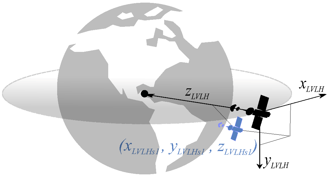
2.1. Coordinate System
The coordinate system used in this paper is the local-vertical, local-horizontal (LVLH) coordinate system as defined by European Space Agency (ESA) and the International Space Station (ISS) program [
21] as shown in
Figure 1. (There are multiple definitions of LVLH with differently labeled axes.)
2.2. Linear Model of Satellite Dynamics
To develop and implement a controller a model, describing the behaviour of the specific system is necessary. In many SFF applications the Hill’s equations [
22] can be used as a good approximation providing a linearized set of equations of motion. Thus they are chosen as the model. In general, they describe the relative motion of a chaser with respect to a leader spacecraft as differential equations. Being an approximation, the Hill’s equations show errors with respect to actual satellite behaviour. Depending on individual accuracy requirements they should only be applied within close range of up to few tens of kilometers and nearly circular orbits with small eccentricities in the order of
. They are given in LVLH as
with
being the mass of the chaser spacecraft and the angular frequency of the leader spacecraft
with
being the Earth’s standard gravitational parameter and
a the semi-major axis of the leader satellite ([
23], p. 40). Since Hill’s equations are a set of time-invariant linear differential equations, they can be expressed in state-space form (
):
with the state vector
and total external accelerations or control vector
([
23], p. 40f).
2.3. Graph Theory Fundamentals
Interconnection topologies between satellites or agents in a distributed control system can most adequately be described using graph theory. Thus the relevant terms and definitions later on used will be introduced.
2.3.1. Graph
A graph (or undirected graph) is an ordered pair
, where
V is a set of vertices (or nodes) and
E is a set of edges (see
Figure 2). Each edge itself is an unordered pair of vertices.
e.g., describes the edge between the vertices
and
. For an undirected graph
[
24].
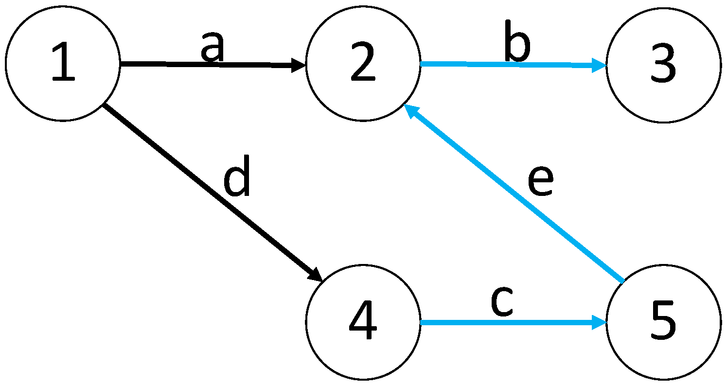
2.3.2. Directed Graph
A directed graph (or digraph) is a graph in which the edges have orientations (see
Figure 3). Thus an edge is an ordered pair of two vertices.
then describes the edge from vertex
to vertex
. In general, for directed graphs
[
24].
2.3.3. Path
A path in a directed graph is an ordered sequence of vertices such that any consecutive pair within the sequence is an edge of the directed graph. In other words, a path is a walk through a graph from a vertex via vertices to a vertex along edges. The length of the path is defined by the number of consecutive edges in the path.
Figure 4 visualizes a path within a graph [
24].
2.3.4. Reachability
A vertex
within a directed graph is said to be reachable from another vertex
, if there exists a path from
to
. A vertex is globally reachable, if there exists a path from every other vertex. A graph is said to be connected (strongly connected in case of directed graphs), if every vertex is globally reachable. Cf.
Figure 4 as an example where vertex 3 is a globally reachable node, since it is reachable from every other vertex [
24].
2.3.5. Neighbor
A vertex
is said to be a neighbor of vertex
, if there exists an edge
from vertex
to vertex
. For undirected graphs, if
is a neighbor of
then also
is a neighbor of
, e.g., in
Figure 4 nodes 2 is a neighbor of node 1, but not the other way round [
24].
2.3.6. Adjacency Matrix
Neighborhood relations within a graph can be expressed in an algebraic way as a matrix, the so called adjacency matrix
with
A graph is undirected, if
[
24].
2.3.7. Degree Matrix
The degree matrix
is a diagonal matrix stating the number of edges connected to each node. It is defined as
where the degree
counts the number of outgoing edges of a vertex
[
24].
2.3.8. Laplacian Matrix
The Laplacian matrix
is a matrix representation of the graph. It combines adjacency and degree matrix and is defined as:
To get a better understanding of its physical meaning we can consider the case that only relative measurement between the agents along the connected edges is available. In this case the relative measurement of agent
i can be written using
as
or in matrix form
Thus it can be understood as a relative-measurement matrix [
24].
2.4. Distributed Control
A distributed control system is a control system wherein individual controllers are distributed throughout a larger system. Thus it differs from non-distributed systems, that consist of a single controller at a central location. In a distributed control system, a set of controllers is connected via a communication network. According to Tian [
24] common features of distributed control systems are distributed interconnections, local control rules, scalability and of course cooperation among the agents. Since in a distributed control system there is no central controller, the cooperation among the agents is crucial for the functionality of the system. Another characteristic is the spatially distributed interconnection of the agents. Each agent/local controller thus does not only take information about its own state/output into account, but also considers the information of some other agents. Since they can be distributed among large distances also delays or package loss may play a role. Distributed control systems feature a local control rule. Because there is no centralized supervisor/controller, each agent makes its own decisions based on its own sensor inputs and the information provided by its neighboring agents. An advantage of a local control rule is the high fault-tolerance capability, since failing of a single or few agents will not stop the complete system from working. Another reason why a local control rule is beneficial is scalability. Since a local control rule uses only local information from the agent itself or from neighboring agents, it usually does not depend on the size of the whole system and thus allows for an arbitrary number of agents in the system. Scalability enables the adaption of the control system towards new applications without changing the underlying system. Further distributed control systems can be differentiated into homogeneous and heterogeneous systems depending on the types and characteristics of the agents, if they are equal or differ [
24].
2.4.1. Connection to Graph Theory
In a distributed control system, the network topology or interconnection scheme can be modeled using directed graphs. Each vertex represents a subsystem or agent. If there is information flow (i.e., a communication link) from one agent to another, then there exists an edge with the same direction in the graph. If all communication links are bidirectional, the topology can be described by an undirected graph.
2.4.2. General State-Space Representation of a Distributed LTI System
A distributed linear time-invariant (LTI) control system
consisting of
N subsystems
can be described as:
and a subsystem
is defined as:
with the time dependencies of
,
,
,
,
,
being omitted to improve readability. (For fundamentals about single LTI control systems the reader is referred to ([
25], p. 72)). The terms
,
,
,
describe the behavior of the subsystem
itself, whereas the mixed terms
,
,
,
describe the influence of other subsystems
on the subsystem
. Thus the coupling terms can be named as
2.4.3. Decentralized and Distributed Control
A controller can be used to compute the control input for the distributed system
described in Equations (
9) and (
10), e.g.,
. If the controller takes only the local state into account, meaning
it is using a decentralized control approach. If it also takes states of other subsystems into account, meaning
it is using a distributed control approach.
2.4.4. Distributed Consensus Approach
There are different types of distributed control systems. A promising way of cooperation in a distributed control system is finding a common agreement or consensus among the agents [
24]. The distributed consensus approach is a method to compute the control input
of distributed systems
in which only the controllers, but not the plants are coupled.
Figure 5 shows an exemplary block diagram for two coupled controllers with these characteristics. With respect to the general representation in Equations (
9) and (
10) the matrices
,
,
and
are equal 0
.
In this case, the control input can then be defined by a consensus protocol (for a regulator problem) by ([
26], p. 26):
where
are the elements of the adjacency matrix
and
K is a gain matrix for a single subsystem/agent. With the state-space definition of a single system
and by linking together the states of the subsystems
to form the state of the overall system the closed-loop system with consensus protocol can be written in matrix form as ([
24], eq. 6.59):
where ⊗ denotes the Kronecker product, an operator on two matrices defined as
with the properties
This control approach enforces the satellites to reduce the relative distances/vectors along all interconnections.
2.4.5. Reference Tracking
The consensus protocol for regulation problems presented in Equation (
13) can be adapted for reference tracking problems:
with
being the reference vector from satellite
i to satellite
j. Obviously,
and
.
Figure 6 shows an exemplary block diagram of three systems with controllers coupled via the consensus approach.
Additionally,
Figure 7 presents a schematic explaining the relative references
provided to the distributed controllers as stated in Equation (
21).
To reformulate Equation (
21) in matrix form the references
can be organized in a matrix:
R is skew-symmetric and has the same zero-values as the adjacency matrix
. Using
R, the closed-loop system of this extended tracking problem can also be written in matrix form:
or
where ⊙ denotes the Hadamard product (or element-wise product) of two matrices, which is defined for two matrices
A and
B with equal size
by
The aim of formation control is that all agents follow a predefined or given trajectory while maintaining a particular spacial formation. Thus, the consensus approach is especially suitable for formation control.
2.4.6. Fixing Coordinate Origin to an Agent
In some cases, e.g., for easier measuring of the states of the involved agents and easier definition of the coordinate frame origin, it makes sense to fix the coordinate frame origin to one agent’s position. This means that the state of this agent, called leader, is always zero. The leader then is passive and no control input should be applied to him to control the internal structure of the formation. To enable this, the interconnection graph has to be directed and the adjacency matrix has to be asymmetric. Connections to the leader are possible, but connections from the leader are forbidden. This leads to the following condition for the elements of an adjacency matrix and a fixed, passive leader l.
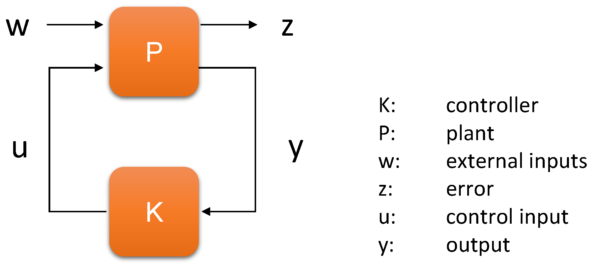
2.5. Robust Control
Robust control is a branch of control theory that explicitly deals with uncertainty. A controller designed for a particular set of parameters is said to be robust, if it would also work well under a different set of assumptions. Rather than adapting to variations of measurements, the controller is designed to work assuming that certain variables will be unknown, but bounded.
loop-shaping is an typical example.
Figure 8 presents a block diagram of a general control configuration in a robust setup.
A generalized plant including external inputs
w, errors
z, control inputs
u and outputs
y can be represented as a general state-space model with the state
x and its derivation
as internal variables:
External inputs
w can contain various inputs from a reference signal
r to disturbances
d to noise
n. The state-space model can be—as every control system expressed in a state-space representation—transformed into a transfer function (TF) ([
27], p. 442), ([
28], p. 20). (The inverse transformation from a TF
to a state-space model
cannot be formulated in a general formula, but is dependent on the order of the system and the number of inputs and outputs. Different procedures can be applied to compute this transformation. Depending on the procedure, either the observability canonical form, controllability canonical form or the diagonalized form of a state-space model can be obtained ([
29], p. 119).) The transformation from a state-space model to a TF can be performed using
as
With the help of Equation (
28), we introduce the notation
which implies Equation (
28) and translates the state-space representation to a TF ([
27], p. 442).
2.5.1. Control
The
control approach considers the
norm of the closed-loop transfer function (CLTF)
with
representing the lower linear fractional transformation (LFT) [
30]. It is defined for a given complex matrix
M and a given rational matrix
with
as
The
control problem can be defined as finding a stabilizing controller that (1) minimizes
(optimal control problem) or (2) with
(suboptimal control problem) ([
27], p. 443).
2.6. Distributed Robust Control
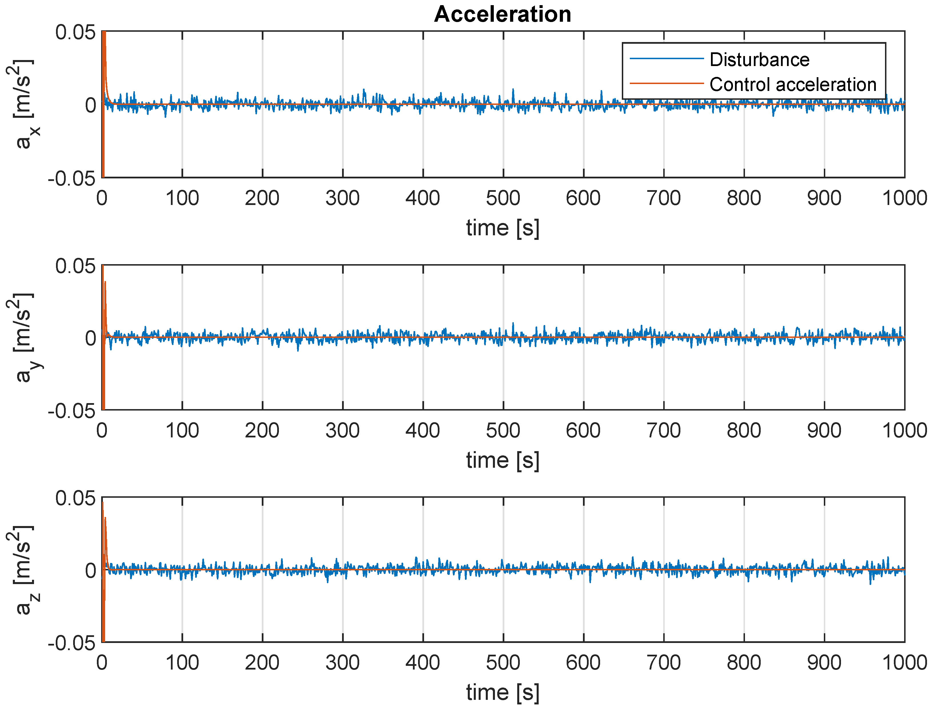
In this section, a combination of distributed control using the consensus approach and robust -control as defined in the previous sections is presented. The main objectives of control are reference tracking for acquiring a given relative formation topology, together with disturbance rejection (e.g., errors of actuator systems) under the presence of (sensor) noise. In addition, the required control input should be optimized. Thus a mixed sensitivity approach is chosen, which is presented in the following section.
2.6.1. Mixed Sensitivity Closed-Loop System with Distributed Controller Interconnections
Based on the work presented in
Section 2.4.4 and in
Figure 6 on the distributed consensus approach and especially on and Equation (
21), which describes the consensus protocol for reference tracking, we first compile a block diagram of the closed-loop system of a single agent
i with mixed sensitivity robustness and an arbitrary number
n of interconnections to other agents’ controllers. This is presented in
Figure 9.
2.6.2. Obtaining Generalized Plant for Single Agent
From the block diagram in
Figure 9 the complete generalized plant for mixed sensitivity with distributed consensus based reference inputs for agent
i with interconnections to
n other agents can be derived:
with
y being the output of agent
i,
d the disturbance and
n the noise.
is the weight on the connection from agent
j to agent
i. In general case
, though in practical applications communication between agents often is bidirectional, which leads to
. Further,
and
is the reference for the relative state from agent
j to agent
i. Further
is assumed here.
2.6.3. Computation of the CLTF
The CLTF
of an agent
i can be computed by combining the generalized plant description given in Equation (
36) with a controller
using a lower LFT. By dividing the overall matrix into four block matrices
Equation (
36) can be reformulated to
The CLTF
can be computed by combining the above matrix and the controller
in a lower LFT:
By introducing the sensitivity
the CLTF can be expressed as
This equation can be simplified using the identities
and
(derived from the definition of the sensitivity function
and the complementary sensitivity function
, cf. ([
29], p. 22)):
By further assuming
(which is equivalent to the fact that
weights connections between agents and not channels individually), we can use the identity
and simplify the element
of
, which is the TF
. Further it is to note that, if
, which means that there is no gain on the connections between the agents, the CLTF simplifies to
which is identical to the classical mixed sensitivity CLTF of a single system (except of the additional reference inputs
and
and renaming
to
).
2.6.4. Obtaining the Generalized Plant for the Overall System
Starting from the plant description of the distributed systems or agents in Equation (
36), we now compose the general plant of the overall system
P. Thus we define
. We further assume that the individual agents are equal. Thus
The general plant description can then be composed of the
of the individual agents under the given assumptions to:
To reduce the size and increase the readability and usability of this matrix, we can combine different parts of it as matrices. Thus we use the Kronecker product ⊗ with its properties defined in Equations (
15)–(
20) and the Hadamard product ⊙ as defined in Equation (
25). Further, let
(this can be understood as the effect of all weights
on the output
of a system
i before entering the controller
) and
and
For better readability we define the unit matrices
and
Now we can rewrite Equation (
43) with inputs and outputs in vector form as
with
n being the number of agents or subsystems and
s the number of states per subsystem (or alternatively
the total number of states of the overall system). Now we have a general plant description of a distributed multi-agent system using consensus control that can be applied to
synthesis.
It has to be noted that the matrix giving the general plant description of the overall system in Equation (
49) grows with the number of agents. Thus using this equation is not suitable for large scale systems with hundreds or thousands of agents, since it will not be possible to find numerical solutions for extremely large matrices. However, Equation (
36) which describes the generalized plant of a single agent only scales with the number of interconnected agents and thus can be used also in large scale systems as long as the number of interconnected neighbors remains small.
4. Discussion
This paper presents a new approach of combining the fields of distributed control and robust control. The distributed consensus approach is related to classical robust control. A generalized plant description including disturbances, noise and a formation topology as target reference has been derived for each single agent in a distributed setup. This plant description is suited to synthesis, which can compute the distributed robust controller. In addition, a generalized plant description describing the overall system is presented as well.
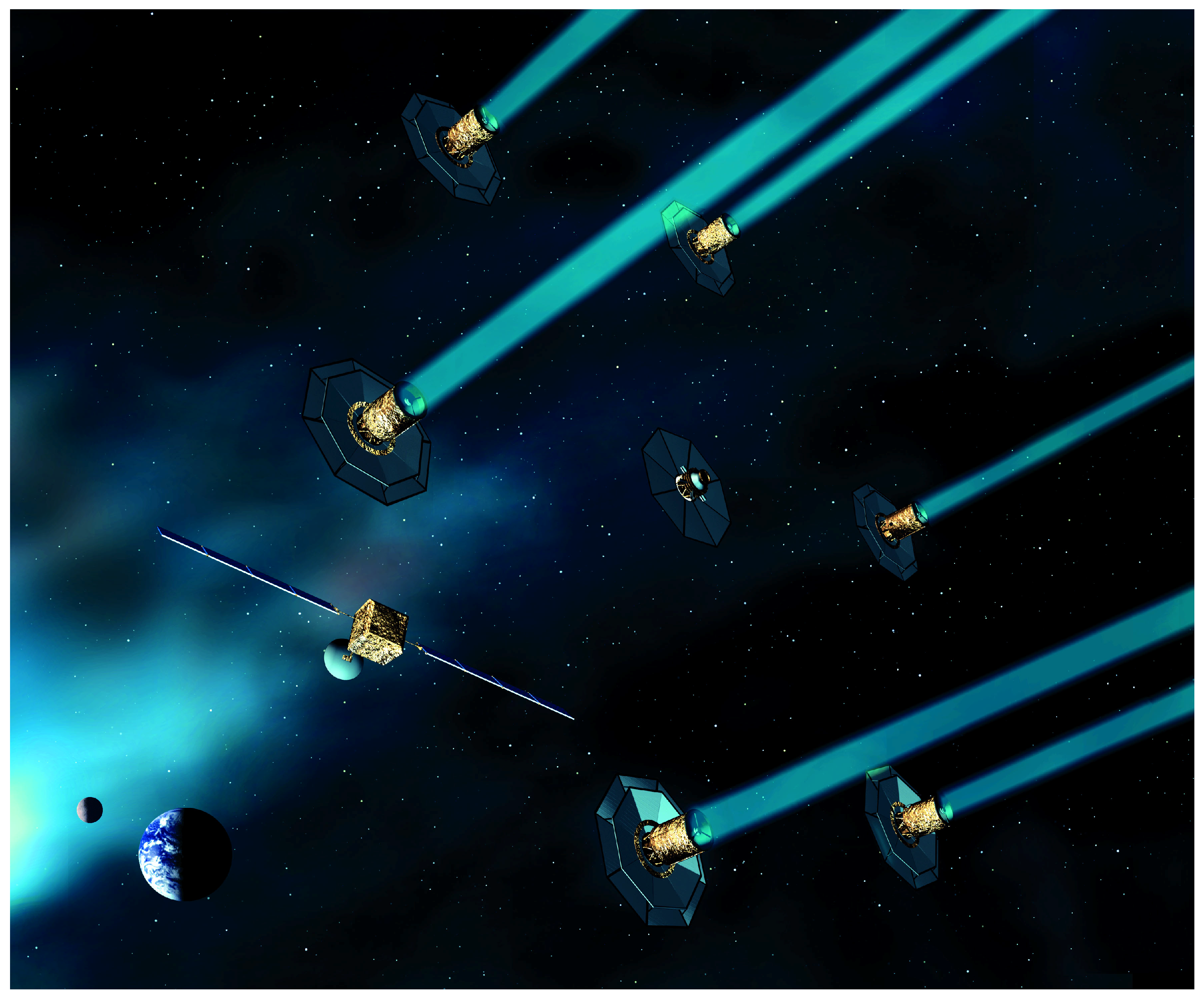
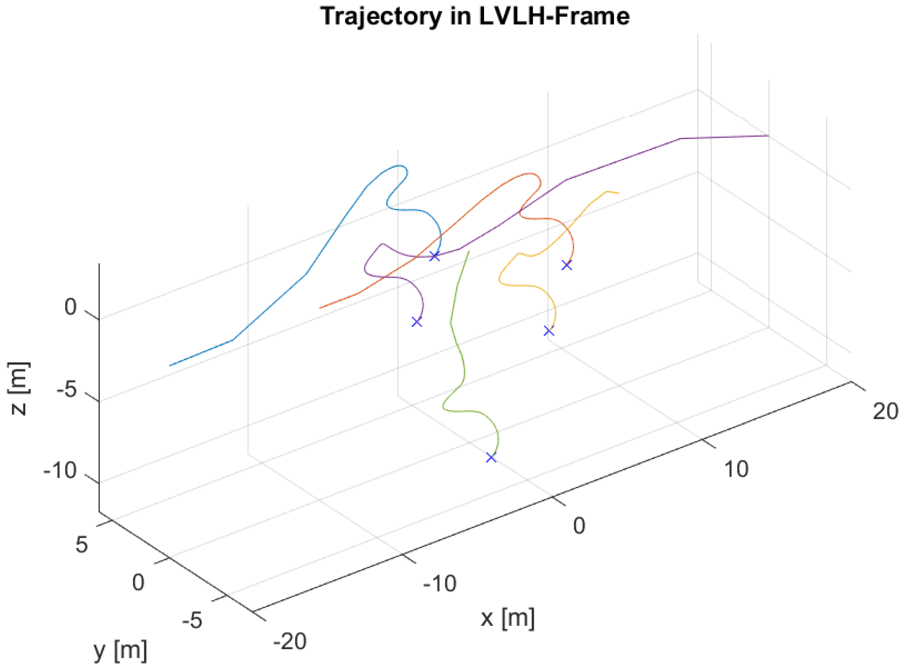
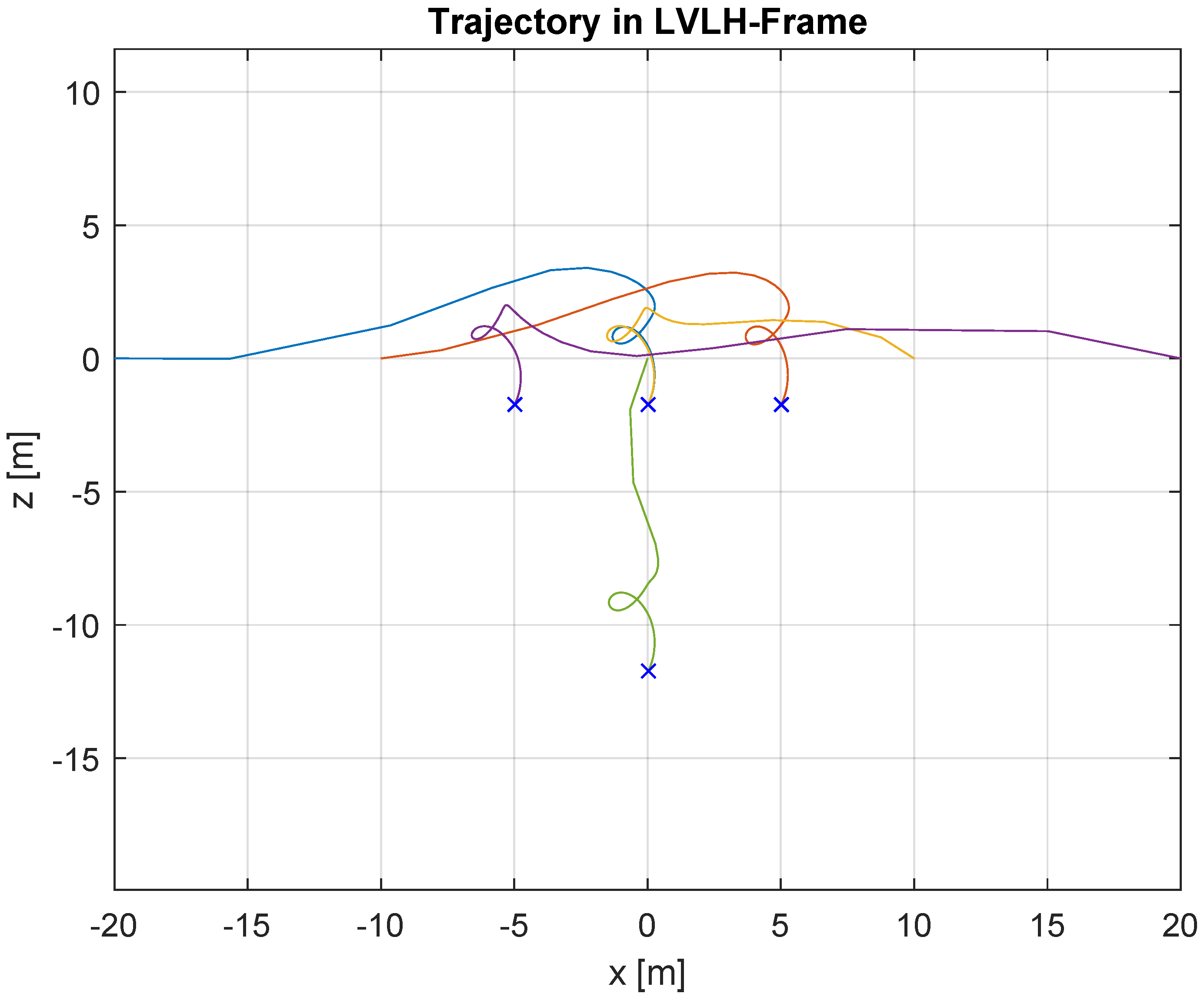
Special focus was set towards space applications, namely satellite formation flying, both during controller design as well as during the simulations. Thus, as scenario a spaceborne distributed telescope has been used. It consists of a 3D formation. Both, convergence towards this formation as well as maintaining it, has been simulated. The simulation results are presented that show the applicability of the developed distributed robust control method to this simple, though realistic space scenario. By using this method, an arbitrary number of satellites/agents can be controlled towards any formation geometry. The developed combination with robust control suffices the high stability and robustness demands of space applications. Of course, this control approach is applicable and beneficial for other application areas as well.
As future work continuing this development the simulations can be extended by adding realistic sensor noise in addition to the implemented disturbances. The simulation of additional scenarios would improve the evaluation of this control approach for further applications. A comparison with other control approaches suiting the presented scenario would help to assess the performance of the presented approach. Additionally, the implementation of collision avoidance would pave the way for a real-world application of this control approach and further broaden the field of possible applications. The implementation of physical constraints (e.g., maximum allowed thrust) would also further improve the presented approach towards real-world applications, since in many cases constraints are required. Last but not least, the implementation and demonstration of this controller in a real-world application would finally prove its applicability. This is planned within the upcoming satellite formation flying mission NetSat.


