An Analysis of the Impact of LED Tilt on Visible Light Positioning Accuracy

Abstract

Whereas the impact of photodiode noise and reflections is heavily studied in Visible Light Positioning (VLP), an often underestimated deterioration of VLP accuracy is caused by tilt of the Light Emitting Diodes (LEDs). Small LED tilts may be hard to avoid and can have a significant impact on the claimed centimeter-accuracy of VLP systems. This paper presents a Monte-Carlo-based simulation study of the impact of LED tilt on the accuracy of Received Signal Strength (RSS)-based VLP for different localization approaches. Results show that trilateration performs worse than (normalized) Least Squares algorithms, but mainly outside the LED square. Moreover, depending on inter-LED distance and LED height, median tilt-induced errors are in the range between 1 and 6 cm for small LED tilts, with errors scaling linearly with the LED tilt severity. Two methods are proposed to estimate and correct for LED tilts and their performance is compared.

1. Introduction

1.1. Introduction on Visible Light Positioning

The introduction of Light Emitting Diodes (LEDs) for traditional lighting applications has also led to new research lines in other application domains, as LEDs can be modulated to transmit information over the visible light propagation channel. Besides large interest in high-speed Visible Light Communication (VLC), another promising application is Visible Light Positioning (VLP) [1,2], where e.g., the location of a photo diode (PD) is estimated. When using Received Signal Strength Indicator (RSSI)-based positioning [3], VLP has an advantage over well-known Radio-Frequency (RF) solutions, thanks to the absence of small-scale fading effects. Research has shed light on the impact of noise on positioning performance [4], the impact of reflections [5,6], or the impact of LED power uncertainty [7]. Also the impact of receiver tilt has been characterized [8,9,10,11], and ways to compensate for this, but it remains unclear to what extent random small tilts of the LED at the ceiling impact positioning performance.

1.2. Expected Issues Considering LED Tilt

Besides tilt induced via the LED die placement and packaging, another important source of tilt is the operator suspending the LED. As suspending a LED is typically done while looking up and standing on a ladder or a hydraulic platform lift, it becomes harder for the operator to maintain a good feeling of horizontality, compared to when standing on the ground. Intuitively, one would expect that the impact of LED tilt on the positioning error strongly relates to the lateral deviation in the receiver plane, defined as the distance between the intersect of the untilted LED normal and the receiver plane (i.e., right below the LED), and the intersect of the tilted LED normal and the receiver plane (i.e., where the LED beam is directed to). This lateral deviation is equal to the tangent of the tilt angle (in radians) multiplied by the LED-PD height difference, or, for small tilt angles, the product of the LED-PD height difference and the tilt angle (in radians) itself. Figure 1a shows the value of this deviation in the receiver plane due to a tilted LED, as a function of the LED height (i.e., the height difference between the LED and the PD). For real-life industrial VLP applications, LED heights of 7 m or more are not uncommon and lead to deviations between 12 cm (for a tilt of 1°) and 61 cm (for a tilt of 5°). This paper will quantitatively and qualitatively investigate the validity of this intuitive assumption. Furthermore, it needs investigation to what extent induced errors of multiple LEDs, each with a certain (unknown) tilt, accumulate or compensate each other.

1.3. Paper Content and Structure

This paper will characterize LED-tilt impact within a typical square VLP configuration by means of a Monte-Carlo simulation, in which it is assumed that each of the four deployed LEDs has a certain unknown (small) horizontal tilt, and a random azimuthal rotation. This way, the cumulative distribution function (cdf) of the positioning error will be constructed for different locations within the test site, and for different localization approaches. Also, the impact of LED tilt will be related with the LED height and inter-LED distance. Finally, a brief exploration is presented towards estimating LED tilt by investigating two tilt estimation methods, which can then be used to adjust model-based RSS-VLP fingerprinting maps, and eventually, reduce positioning errors. The remainder of this paper is structured as follows. Section 2 will present the visible light channel model that will be used in the positioning algorithm, the simulation configuration, the positioning algorithms, and the proposed LED tilt estimation methods. In Section 3, the results will be presented, after which the main findings of this work will be discussed in Section 4, together with related future research work.

2. Materials and Methods

2.1. Channel Model

In this work, only the Line-of-Sight (LoS) path between the LED transmitters and the PD receivers are accounted for. We will not consider the impact of reflections as a source of “noise”, in order to be able to unambiguously assess the effect of LED tilt only. For the same reason, no shot noise or thermal noise will be considered in this study. It should be noted that even when reflections are accounted for via a model-based fingerprinting approach [6], LED tilt will have an impact since the reflected contributions could either increase or decrease, depending on the LED location and tilt, the PD location, and the location of the reflective surface. This is considered to be future work. Figure 2 and

Table 1. Summary of the parameters defined in Figure 2.

Parameter	Explanation	Parameter	Explanation
$\theta$	horizontal LED tilt	h	LED-PD height difference
$\alpha$	azimuthal rotation of tilted LED normal	d	LED-PD distance
$\varphi$	general notation for angle of irradiance (=$\phi$ or ${\phi }_{tilt}$)	${\overrightarrow{v}}_{LED2PD}$	vector from LED to PD
$\phi$	angle of irradiance for untilted LED	${\overrightarrow{n}}_{LED}^{notilt}$	untilted LED normal
${\phi }_{tilt}$	angle of irradiance for tilted LED	${\overrightarrow{n}}_{LED}^{tilt}$	tilted LED normal
$\psi$	angle of incidence	${\overrightarrow{n}}_{PD}$	PD normal

define the model parameters of the visible light channel. The power $P_R$ received at the PD is calculated according to the channel model used in [12]:

$$P_R=P_E·h_{LoS},$$

(1)

with $P_E$ the emitted optical power by the LED. $h_{LoS}$ is the channel gain along the direct link and can be described as follows, when assuming a Lambertian radiator:

$$h_{LoS}=\frac{m+1}{2\pi d^2}co{s}^m(\varphi )·A_R·cos(\psi )·T_R(\psi )·G_R(\psi ),$$

(2)

with m the order of the Lambertian emitter, and $\varphi$ the angle of irradiance (i.e., the angle between the LED normal and the vector ${\overrightarrow{v}}_{LED2PD}$ from the LED to the PD, with $\varphi$ equal to either ${\phi }_{tilt}$ or $\phi$ in Figure 2, depending on the LED being tilted or not). $T_R(\psi )$ and $G_R(\psi )$ are the optical filter’s gain and the optical concentrator’s gain at the receiver, respectively, with $\psi$ the angle of incidence (i.e., the angle between the PD normal ${\overrightarrow{n}}_{PD}$ and the vector from the PD to the LED). The LEDs will be assumed to be within the field-of-view (FOV) of the PD and $T_R(\psi )$ and $G_R(\psi )$ are assumed equal to 1. d is the distance between the LED and the PD, and $A_R$ the actual PD area, here assumed to be 1 ${\mathrm{cm}}^2$. The PD will be assumed to be horizontally oriented, so that $cos(\psi )$ reduces to $h/d$, with h the height difference between the LED and the PD.

When the LED is not tilted (i.e., horizontally oriented), the angle of irradiance $\varphi =\phi =\psi$ (see Figure 2) with $cos(\phi )$ also equal to $h/d$. However, in case of LED tilt, the angle of irradiance $\varphi$ is equal to ${\phi }_{tilt}$ (see Figure 2), with $cos({\phi }_{tilt})$ as follows:

$$cos({\phi }_{tilt})=\frac{{\overrightarrow{v}}_{LED2PD}·{\overrightarrow{n}}_{LED}^{tilt}}{|{\overrightarrow{v}}_{LED2PD}|·|{\overrightarrow{n}}_{LED}^{tilt}|},$$

(3)

with ${\overrightarrow{n}}_{LED}^{tilt}$ the (tilted) LED normal (compared to ${\overrightarrow{n}}_{LED}^{notilt}$, being the untilted LED normal). The LED is assumed to be tilted over an angle $\theta$ (determining the severity of the tilt), and rotated over an angle $\alpha$ (determining where the LED is tilted to), as shown in Figure 2. Since $|{\overrightarrow{n}}_{LED}^{tilt}|=1$ and $|{\overrightarrow{v}}_{LED2PD}|=d$, $cos({\phi }_{tilt})$ is obtained as follows:

$$cos({\phi }_{tilt})=\frac{(x_{PD}-x_{LED})sin(\theta )cos(\alpha )+(y_{PD}-y_{LED})sin(\theta )sin(\alpha )+hcos(\theta )}{d},$$

(4)

with $(x_{PD},y_{PD},0)$ and $(x_{LED},y_{LED},h)$ the coordinates of the PD and the LED respectively. Please note that the assumption of the PD being located in the xy-plane, does not retract from the generality of the work, as only the LED-PD height difference h matters.

As such, the power $P_R^{tilted}$ received from a tilted LED on a horizontally oriented PD is calculated as follows:

$$P_R^{tilted}=P_E\frac{h(m+1)A_R}{2\pi d^4}{((x_{PD}-x_{LED})sin(\theta )cos(\alpha )+(y_{PD}-y_{LED})sin(\theta )sin(\alpha )+hcos(\theta ))}^m$$

(5)

2.2. Simulation Configuration

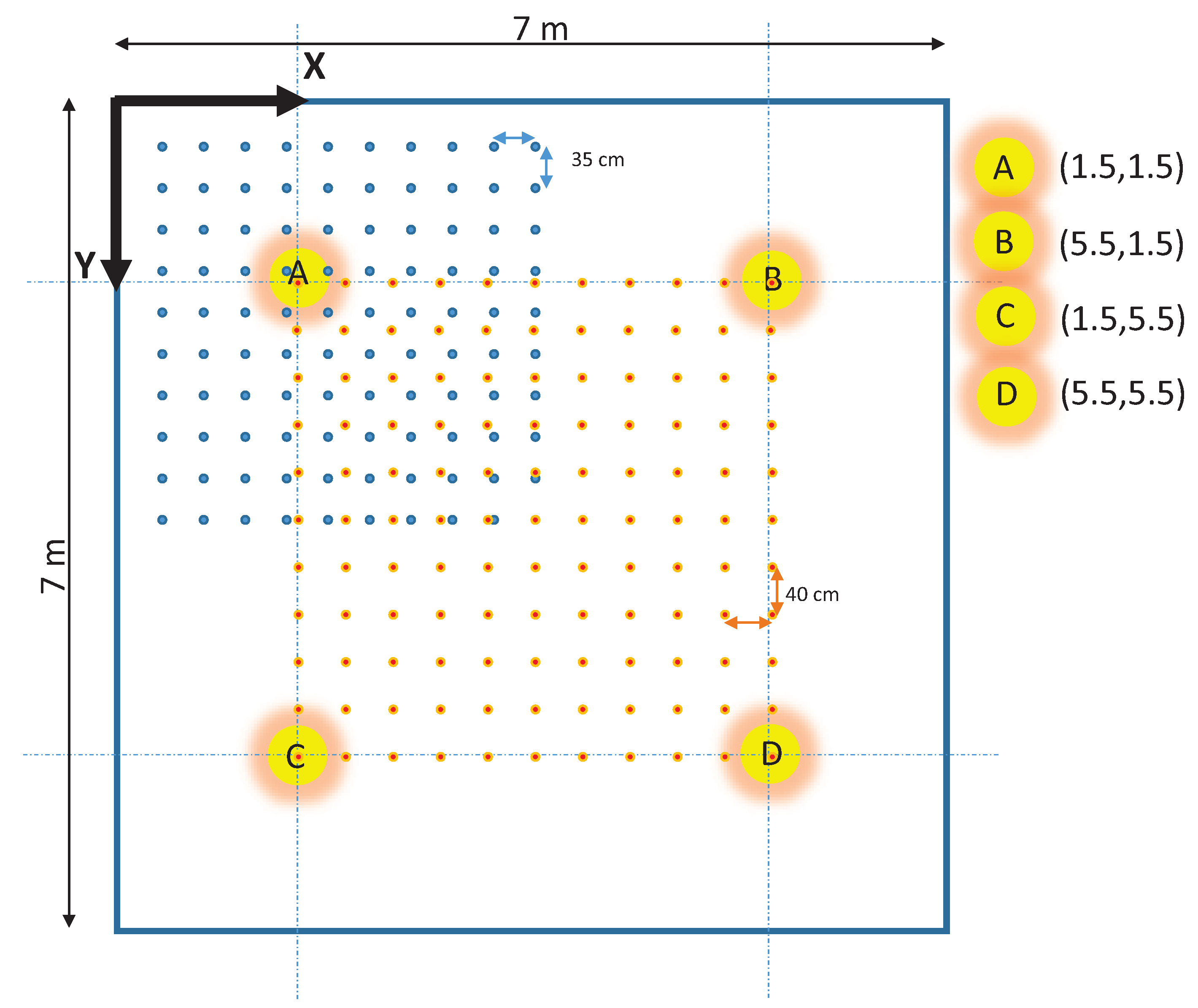
Simulations will be executed for the room depicted in Figure 3. The dimensions of the room are 7 m × 7 m, with a ceiling at a height difference h above the PD, with h = 2.5 m (office environment) or h = 6 m (industrial environment). The Lambertian order m of the LEDs is equal to 1, for all four LEDs. In this scenario, we assume that the receiver height is fixed and known (e.g., a PD attached to the top of a cart), so the evaluation of the receiver location is reduced to a plane. A receiver grid of 5 mm will be considered here, meaning that the PD center can be located at $N_L$ = ${1401}^2$ candidate locations. Furthermore, we assume that the receiver hardware is able to demultiplex the contributions of the different LED sources [13]. Four LEDs are attached to the ceiling, at the locations indicated in Figure 3. We here assume the frequency division multiple access (FDMA) scheme proposed in [13] and further investigated in [14], which combines the transmission of square waves with ‘power spectrum identification’ based on the Fast Fourier Transform of the incident signal. The authors make use of the even harmonics of square waves being zero, to separate the different contributions of each LED transmitter at the receiver side. The modulation frequencies are typically in the range of 1–100 kHz, which is sufficiently below the LED and LED driver bandwidth (>1 MHz) to not have a detrimental impact on the positioning system. Although the exact optical power of the LEDs does not impact the findings, as no receiver noise is added, we here assume an optical power of 10 W, in line with common assumptions in literature [15,16].

The parameter $\theta$ is assumed to be the absolute value of a normally distributed variable ${\theta }_N$, and $\alpha$ to be uniformly distributed: $\theta =|{\theta }_N|$, with ${\theta }_N\sim \mathcal{N}(0,{\sigma }_{tilt}^2)$ and $\alpha =U[0°,360°]$. Two values of ${\sigma }_{tilt}$ will be mainly considered in this work: 1° and 2°, meaning that 95% of the LEDs will be mounted with a tilt below 2° and 4° respectively.

The positioning error due to tilt will be evaluated at 100 locations in a quarter of the receiver plane, i.e., at the blue locations indicated in Figure 3. Thanks to the symmetry of the setup, the resulting error distributions can be extrapolated to the three other zones, since the distribution of the positioning errors will repeat themselves at the corresponding locations of the different parts of the 7 m × 7 m area. It should be noted though that each single simulation will result in an asymmetric setup, since for each simulation, the tilt of each LED will be randomly and independently chosen. However, the resulting cdf at corresponding locations will be the same when a sufficient number of simulations is considered, due to the fact that the statistical distribution of the LED tilt is assumed to be the same for each of the LEDs. In this work, a position estimation for each of the 100 positions will be executed for 10,000 random sets of LED tilts in a Monte-Carlo simulation. Each position estimation will be done according to the algorithms presented in Section 2.3.

2.3. Positioning Algorithms

Three different positioning algorithms will be compared: a traditional trilateration method, and two model-based fingerprinting methods using a Least-Squares Estimation (LSE) and a normalized LSE (nLSE) respectively.

2.3.1. Trilateration

Given a measured power $P_{Ri}^{meas}$ from $LE{D}_i$ (i = 1..N) and assuming that $cos(\varphi )$ = $cos(\psi )$ = $\frac{h}{d_i}$ for horizontally oriented LEDs and PD (see Figure 2), Equation (2) can be rewritten to allow the calculation of the estimated distance $\widehat{d_i}$ between $LE{D}_i$ and PD:

$$\widehat{d_i}=\sqrt[m+3]{(m+1)·\frac{P_E}{2\pi P_{Ri}^{meas}}·h^{m+1}·A_R},$$

(6)

The real squared horizontal distance $d_i^2$ between $LE{D}_i$ and the PD is given by:

$$d_i^2={(x-x_i)}^2+{(y-y_i)}^2=x^2-2x{x}_i+x_i^2+y^2-2y{y}_i+y_i^2,$$

(7)

with $(x,y)$ the PD location, and $(x_i,y_i)$ the coordinates of $LE{D}_i$. After eliminating the quadratic terms in $x^2$ and $y^2$ by subtracting $d_N^2$ from $d_i^2$, N-1 equations are obtained (i = 1, …, N − 1):

$$d_i^2-d_N^2=-2x(x_i-x_N)+x_i^2-x_N^2-2y(y_i-y_N)+y_i^2-y_N^2$$

(8)

These linear equations in x and y can be written as b = M $\left[\begin{array}{c}x\\ y\end{array}\right]$, where

$$\mathit{b}=\left[\begin{array}{c}{d}_1^2-x_1^2-y_1^2-d_N^2+x_N^2+y_N^2\\ d_2^2-x_2^2-y_2^2-d_N^2+x_N^2+y_N^2\\ ⋮\\ d_{N-1}^2-x_{N-1}^2-y_{N-1}^2-d_N^2+x_N^2+y_N^2\end{array}\right]$$

(9)

$$\mathit{M}=\left[\begin{array}{cc}{x}_1-x_N& y_1-y_N\\ x_2-x_N& y_2-y_N\\ ⋮& ⋮\\ x_{N-1}-x_N& y_{N-1}-y_N\end{array}\right]$$

(10)

$\left[\begin{array}{c}x\\ y\end{array}\right]$ can then be estimated as $\left[\begin{array}{c}\widehat{x}\\ \widehat{y}\end{array}\right]$ using the Moore-Penrose pseudo-inverse of M:

$$\left[\begin{array}{c}\widehat{x}\\ \widehat{y}\end{array}\right]={({\mathit{M}}^{\mathit{T}}\mathit{M})}^{-1}{\mathit{M}}^{\mathit{T}}\mathit{b}$$

(11)

In case the LEDs are tilted, the assumption of $cos(\varphi )$ = $cos(\psi )$ = $\frac{h}{d_i}$ will no longer hold, and errors will be introduced.

2.3.2. Least-Squares Estimation

The following two methods are based on the comparison of the set of so-called measured received powers $P_{Ri}^{meas}$ from each (tilted) $LE{D}_i$ (i = 1, …, N) at the unknown PD location $(x_{PD},y_{PD})$, with the set of fingerprinted PD powers $P_{Ri}^{L,model}$ from $LE{D}_i$ at all (${1401}^2$) locations L in the grid. For the construction of the fingerprinting database of the $P_{Ri}^{L,model}$ values, each LED is assumed to be untilted, as it is its most probable position. The set of so-called measurements ($P_{R1}^{meas},P_{R2}^{meas},\dots ,P_{RN}^{meas}$) represent the observed values in the realistic setup investigated here. They are obtained from ($P_{E1},P_{E2},\dots ,P_{EN}$), where $P_{Ri}^{meas}$ values are obtained from Equation (5) with $\theta$ and $\alpha$ values as samples from their respective statistical distributions. The larger the tilt of the LEDs (larger ${\sigma }_{tilt}^2$ values), the larger the positioning errors will be. The algorithm estimates the unknown location with coordinates $(x_{PD},y_{PD})$ to be at the location L where the Least-Squares cost function $C_{LSE}^L$ has a minimum [6]:

$$C_{LSE}^L=\sum _i^N{(P_{Ri}^{meas}-P_{Ri}^{L,model})}^2.$$

(12)

2.3.3. Normalized Least-Squares Estimation

The normalized Least-Squares Estimation algorithm was shown to perform better than the LSE algorithm when there is uncertainty on the respective LED powers [17]. The unknown location $(x_{PD},y_{PD})$ is estimated at the the location L where the cost function $C_{nLSE}^L$ has a minimum:

$$C_{nLSE}^L=\sum _i^N{(\frac{P_{Ri}^{meas}-P_{Ri}^{L,model}}{P_{Ri}^{L,model}})}^2.$$

(13)

For the LSE and nLSE methods, each position estimation thus consists of a comparison of the set of measurements ($P_{R1}^{meas},P_{R2}^{meas},\dots ,P_{RN}^{meas}$) against all ($P_{R1}^{L,model},P_{R2}^{L,model},\dots ,P_{RN}^{L,model}$) sets that are stored in the database. In total, $N_L$ sets of N values of $P_{Ri}^{L,model}$ are precalculated and stored in a fingerprinting database, i.e., the received power at $N_L$ locations from each of the N LEDs, according to the LoS channel model from Section 2.1. For the configuration under test, N = 4 and $N_L$ = ${1401}^2$ = 1,962,801, meaning that 7,851,204 values are stored.

2.4. LED Tilt Estimation Methods

Based on the configuration and the algorithms described in the previous sections, the impact of LED tilt will be assessed. In this section, two methods for estimating the LED tilt are presented, i.e., the angles $\theta$ and $\alpha$ from Figure 2. Once this tilt is known, the fingerprinting map with powers ($P_{Ri}^{L,model}$ values of Section 2.3.2 and Section 2.3.3) can be adjusted, in order to reduce aforementioned LED tilt impact.

2.4.1. Exhaustive Search

The first method encompasses an exhaustive search over all possible $(x,y)$ locations in the receiver plane. As Equation (2) can be rewritten as

$$P_R(x,y)=P_E·\frac{m+1}{2\pi d^2(x,y)}co{s}^m(\varphi )(x,y)·A_R·cos(\psi )(x,y)·T_R(\psi )(x,y)·G_R(\psi )(x,y),$$

(14)

the location ($x_L$,$y_L$) in the receiver plane which is pointed to by the LED normal, can be determined as the (x,y) location for which the angle of irradiance $\varphi$ is minimal or $co{s}^m(\varphi )(x,y)$ is maximal. For a horizontal PD, and when removing all (x,y)-independent factors, ($x_L$,$y_L$) is thus found at the location (x,y) where

$$\frac{P_R(x,y)·d^3(x,y)}{T_R(\psi )(x,y)·G_R(\psi )(x,y)}$$

(15)

is maximal. Especially for small LED tilt values, it is fair to assume that the optical filter’s gain and the optical concentrator’s gain at the receiver are also independent of the receiver location, so that the LED tilt is determined by the location ($x_L$,$y_L$) where the product of the measured received power $P_R(x,y)$ and the cube of the LED-PD distance becomes maximal, i.e.,

$$(x_L,y_L)=\underset{(x,y)}{max}(P_R(x,y)·d^3(x,y)).$$

From the location ($x_L$, $y_L$), the tilt values ($\alpha ,\theta$) are easily derived using basic trigonometry as ($arctan\frac{y_L}{x_L}$, $arctan\frac{\sqrt{x_L^2+y_L^2}}{h}$). Although this method in principle delivers the exact LED tilt, it is very cumbersome, as it requires the execution of a large set of measurements, whereby the exact ground truth of the measurement location has to be known. The measurement campaign should be executed with an automated positioning system, e.g., with a stepping motor [18].

2.4.2. Quick Search

Unlike in the case of the first method, the second method, denoted here as ’quick search’, uses a power measurement at only a limited set of $N_M$ locations under the considered LED. Based on these power measurements $P_i^{meas}$, a minimum-search in the ($\theta$,$\alpha$) space is executed for finding the most likely values for these tilt parameters. We propose a cost function using power ratios at the different locations instead of absolute power values, since the expected powers $P_i^{model}$ are sometimes not known without doing a calibration phase like e.g., in [19]. This is due to e.g., unknown deviations of the assumed LED power, PD responsivity,… When working with power ratios and thus excluding these unknown factors to a certain extent, the cost function is expected to be better suited to identify power differences that are solely due to the LED tilt. As such, the proposed cost function is the following:

$$C_{tilt}(\alpha ,\theta )=\sum _{i=1}^{N_M}\sum _{j=i+1}^{N_M}{\left(\frac{P_i^{meas}}{P_j^{meas}}-\frac{P_i^{model}(\alpha ,\theta )}{P_j^{model}(\alpha ,\theta )}\right)}^2,$$

(16)

with $N_M$ the number of measurement locations in the receiver plane, and $P_i^{meas}$ the measured power at location i underneath the considered LED. The power values $P_i$, i=1..$N_M$, are first sorted in descending order. $P_i^{model}(\alpha ,\theta )$ is the modeled received power at location i, according to Equation (5) for a LED tilt determined by ($\alpha ,\theta$). The cost function iterates over $\alpha$ between 0° and 360°, with a 1° resolution. The parameter $\theta$ is iterated between 0° and ${\theta }_{max}=5°$, with 0.1° resolution. $C_{tilt}$ will reach its minimal value for ($\alpha ,\theta$) values equal to the actual LED tilt values, although the outcome will be corrupted by external factors such as noise, unaccounted PD tilt, deviations from the tabulated Lambertian order.

2.4.3. LED Tilt Estimation Scenario

The performance of the described methods will be evaluated for a 10 W LED at a height of 2.5 m above the receiver plane. The LED is assumed to have a horizontal tilt of $\theta$ = 1.6° and an azimuthal rotation $\alpha$ of 230°. For the ’quick search’ method, four measurement locations ($N_M$ = 4) in the receiver plane will be considered, with (quite randomly chosen) coordinates (1,0), (−0.5,$\pm \frac{\sqrt{3}}{2}$), and (1, −1). Finally, a PD area of $A_R$ = 1 ${\mathrm{cm}}^2$ is assumed.

3. Results

3.1. Assessment of LED Tilt Impact on Positioning Accuracy for Typical Configurations Using Different Metrics

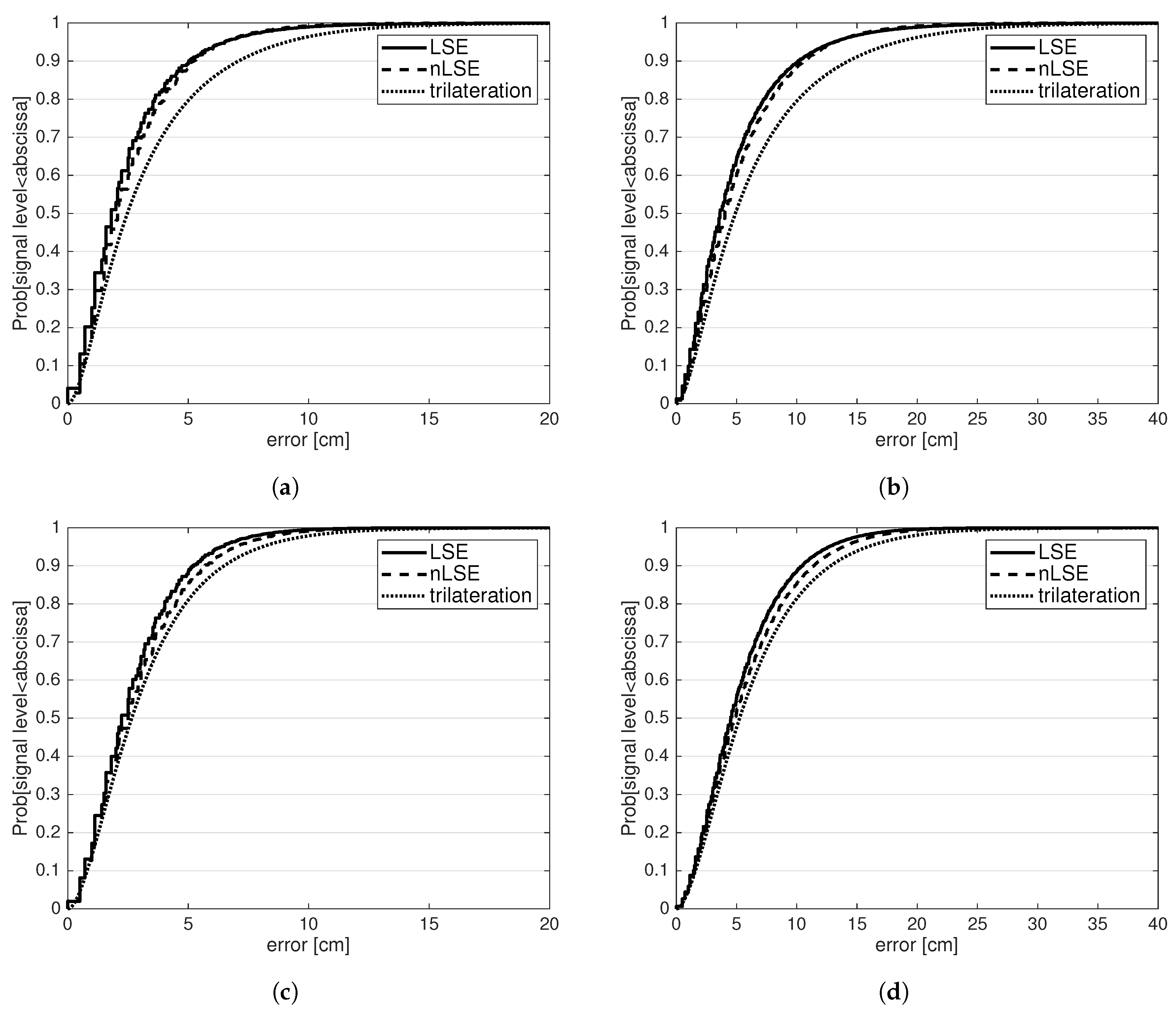
Figure 4 shows the cdf of the positioning errors of the ${10}^4$ simulations at each of the 100 evaluation locations for (a) a LED-PD height difference of 2.5 m and ${\sigma }_{tilt}$ = 1° (denoted as normal office placement); (b) a LED-PD height difference of 2.5 m and ${\sigma }_{tilt}$ = 2° (denoted as sloppy office placement); (c) a LED-PD height difference of 6 m and ${\sigma }_{tilt}$ = 1° (denoted as normal industrial placement); and (d) a LED-PD height difference of 6 m and ${\sigma }_{tilt}$ = 2° (denoted as sloppy industrial placement). In each plot, the three localisation metrics from Section 2.3 are compared.

Table 2. Median and maximal positioning errors for the three localization approaches, for four typical LED deployments.

Positioning Error (cm)	LSE		nLSE		Trilateration
	$p_{50}$	$p_{95}$	$p_{50}$	$p_{95}$	$p_{50}$	$p_{95}$
normal office (h = 2.5, ${\sigma }_{tilt}$ = 1°)	1.80	6.52	2.06	6.52	2.47	9.07
sloppy office (h = 2.5, ${\sigma }_{tilt}$ = 2°)	3.64	13.09	4.03	13.15	4.90	18.35
normal industrial (h = 6, ${\sigma }_{tilt}$ = 1°)	2.24	6.40	2.50	7.02	2.66	8.08
sloppy industrial (h = 6, ${\sigma }_{tilt}$ = 2°)	4.53	12.65	4.92	13.87	5.25	15.87

lists the median ($p_{50}$) and 95%-percentile ($p_{95}$) values of the errors for the different configurations. It is observed that for a normal office placement (see Figure 4a), median errors are around 2–3 cm and 95-percentile errors between 6 and 10 cm. The LSE metric slightly outperforms the nLSE metric, whereas traditional trilateration produces errors that are almost 40% higher on average than for LSE. For a sloppy industrial placement (see Figure 4b), median ($p_{50}$) and maximal ($p_{95}$) errors more or less double, compared to the normal placement, for all metrics.

When increasing the height to 6 m (industrial), errors increase, but not significantly. For a normal industrial placement (see Figure 4c), although median errors increase between 8 (trilateration) and 24% (LSE) compared to the normal office placement, maximal errors even see a slight decrease for the LSE and trilateration approaches. The next section will elaborate on this impact of LED height more thoroughly. Finally, for a sloppy industrial placement (see Figure 4d), the errors again more or less double compared to the normal industrial placement, suggesting that doubling ${\sigma }_{tilt}$ for each of the LEDs also doubles the resulting positioning error.

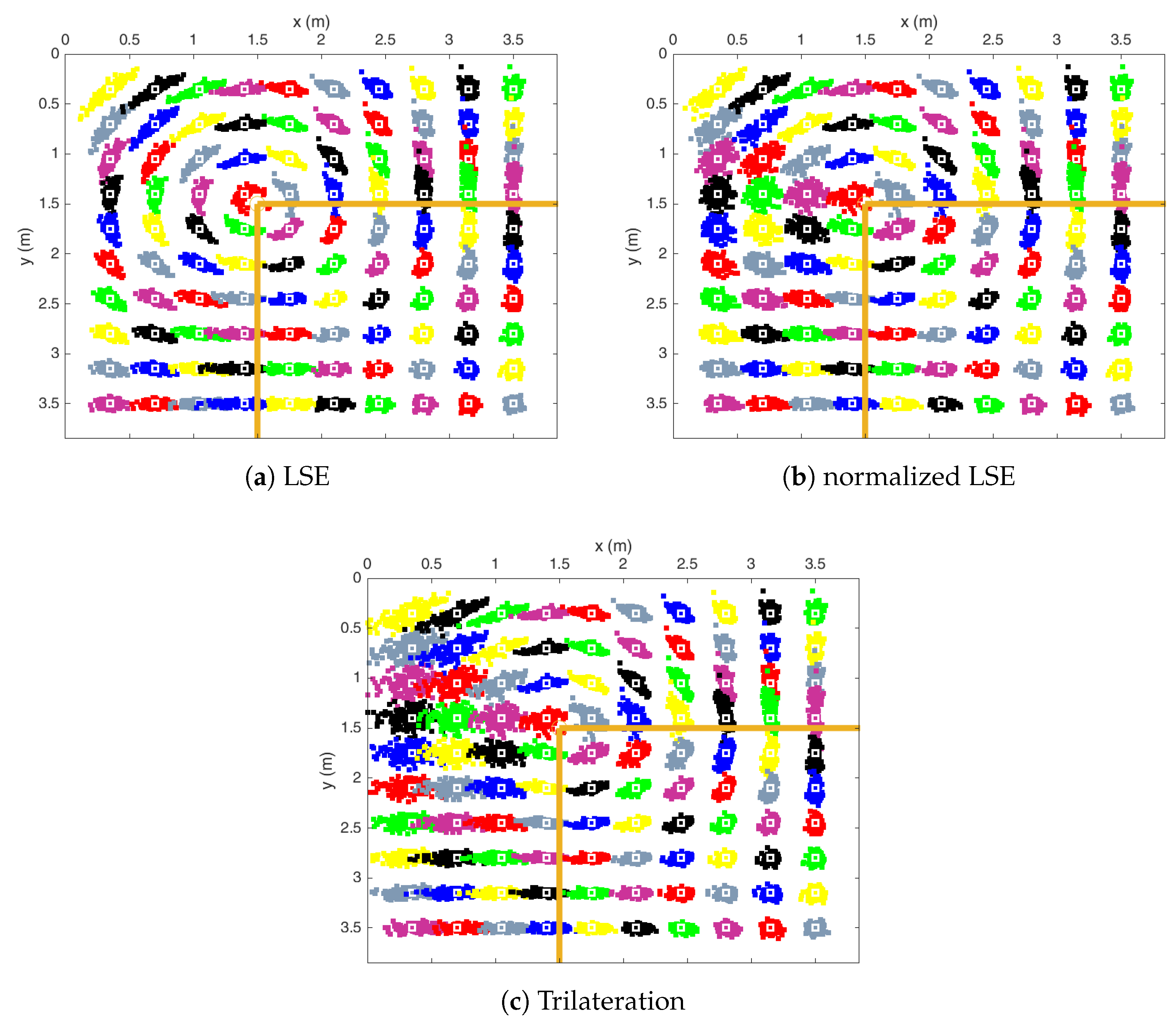
To give more insight on the spatial distribution of the postion estimates for the different localization approaches, Figure 5a–c show a scatter plot of the estimated positions for a LED-PD height difference of 2.5 m, and a ${\sigma }_{tilt}$ value of 2°, for LSE, nLSE, and trilateration, respectively. For each of the 100 evaluation points, 250 estimations are displayed. These 100 evaluation points correspond to the blue dots in Figure 3. The square that is formed by the LEDs is partly shown with orange lines. These scatter plots correspond to the values in Table 2 for a ’sloppy office’ deployment. The dominant LED at (1.5, 1.5) causes a more circular pattern due its LED tilt for the LSE metric than for nLSE, showing that nLSE indeed reduces the impact of the dominant LED. Trilateration performs worse than the other two metrics, but especially outside the LED square (i.e., for x or y coordinates <1.5 m). Inside the LED square, the performance of the algorithms is comparable.

3.2. LED Tilt Impact for Different Inter-LED Distances, LED Height and Tilt

In this section, we further characterize the errors due to random LED tilt, using the common trilateration method described in Section 2.3.1. Different configurations with four LEDs in a square configuration are investigated. We vary the side of the square (i.e., the inter-LED distance) between 2 and 8 m in steps of 1 m, the LED height between 2 and 8 m in steps of 1 m, and ${\sigma }_{tilt}$ between 1 and 3° in steps of 1°. For each of these 7 × 7 × 3 =147 combinations, each of the 4 LEDs are randomly tilted and the localisation accuracy is evaluated on a uniform 11 × 11 grid in between the LED locations, meaning that the accuracy is evaluated only inside the LED square, for which was observed that all three localization approaches yielded comparable estimation clouds (see Figure 5). These 121 evaluation points correspond to the orange dots in Figure 3. Please note that Figure 3 represents a configuration with square side length S = 4. For each of the 147 combinations, 5000 LED tilt settings are generated, with the LEDs tilted according to the statistical tilt distributions presented in Section 2.2. As (thermal or shot) noise is not considered here, the value of the transmit power $P_E$ or the PD area $A_R$ has no influence on the positioning accuracy, so conclusions are also valid for other LED optical powers or PD areas.

Figure 6a shows the $p_{50}$ error due to LED tilt for 7 different square side lengths (2 to 8 m), as a function of the LED height, for a ${\sigma }_{tilt}$ value of 1°. The figure shows that irrespective of the LED height, the impact of tilt is the lowest for smaller LED squares. e.g., for a LED height of 2 m, the median induced positioning error increases from 1 cm for a 2 × 2 m LED square to 6.5 cm for an 8 × 8 m LED square. As the LED height increases, the influence of the square side length reduces, with median errors between 2.4 cm (2 × 2 m square) and 3.8 cm (8 × 8 m square). Furthermore, it is interesting to note that the impact of LED tilt on positioning accuracy in the receiver plane does not necessarily increase with LED height (i.e., higher LED-PD height differences), while intuitively (and from Figure 1a), one might expect a monotonic increase of the induced error with LED height. However, for a given LED square size S, there appears to be an optimal LED height with respect to the impact of LED tilt. e.g., for an 8 × 8 m LED square, this optimal LED height is 6 m, decreasing to 4 m for a 5 × 5 m LED square, and to smaller than 2 m for a 2 × 2 m LED square.

We explain this using Figure 1b, where a 1D-simplified side view of the considered configuration is shown, with h the LED-PD height difference and S the LED square side length. With $\gamma$ between 0 and 1, $\gamma S$ indicates the range of possible lateral displacements L = $h·tan\varphi$ of the PD in the receiver plane, with respect to perpendicular irradiance ($\gamma =0$ is below the LED, $\gamma =1$ is below an adjacent LED of the LED square). $\varphi$ is the angle of irradiance for an untilted LED. The variable of interest here is $\frac{\partial L}{\partial \varphi }$, indicating the additional lateral displacement in the receiver plane, due to a LED tilt $\partial \varphi$: $\frac{\partial L}{\partial \varphi }=\frac{h}{co{s}^2\varphi }=h+\frac{{\gamma }^2{S}^2}{h}$. The result comprises two opposed phenomena. One the one hand, we observe that larger LED heights h correspond to larger additional displacements in the receiver plane. This corresponds to the phenomenon described in Section 1.2 and Figure 1, and is is reflected by the first factor h of $\frac{\partial L}{\partial \varphi }$, meaning that the tilt impact is smaller for smaller LED heights. On the other hand, we see that for a given (and fixed) LED square size S, relatively more receiver locations will have a large angle of irradiance $\varphi$ when h is smaller (see also Figure 1b), leading to a larger additional lateral displacement. This is reflected by the second factor $\frac{{\gamma }^2{S}^2}{h}$ of $\frac{\partial L}{\partial \varphi }$. The combination of these two opposed phenomena causes, depending on the size of the LED square S, the minimal tilt impact to be observed at different height differences h. When the LED-PD height difference is equal to the inter-LED distance (h = S), forming a cube, the error sees a perfect linear increase with h, as indicated by the red curve in Figure 6a, again corresponding to the intuitive assumption described in Section 1.2 ($\frac{\partial L}{\partial \varphi }$ reduces to $h(1+{\gamma }^2)$ for this simplified 1D-case).

Finally, it was again observed that $p_{95}$ errors scale approximately to values equal to three times the $p_{50}$ values. Similarly, the $p_{50}$ errors scale also linearly with the ${\sigma }_{tilt}$ value, as is shown in Figure 6b, depicting the induced median error for a 4 × 4 m LED square, as a function of LED height for three ${\sigma }_{tilt}$ values.

3.3. Evaluation of LED Tilt Estimation Methods

In this section, the performance of the LED tilt estimation methods presented in Section 2.4 are presented. Figure 7a,b show the $P_R·d^3$ values in the receiver plane without receiver noise and with added noise to the received powers (${\sigma }_{noise}$ = ${10}^{-7}$ W) respectively (’exhaustive search method’). The figures indicate the LED location (green asterisk in (0,0)), the real (black asterisk) and estimated (red asterisk) intersect of the LED normal with the receiver plane, and the location receiving the maximal power $P_R$ (blue asterisk). It should be noted that the direction of the tilted LED normal is indeed not only determined by the maximal received power $P_R$ (blue asterisk), as this maximal-power location is determined by a tradeoff between being located along the LED normal (pulling towards the black asterisk) and having the shortest distance to the LED (pulling the location back towards right underneath the LED, green asterisk). This is also why the tilted LED normal intersect is not found at the location with a maximal $P_R$, but instead at the location with a maximal $P_R·d^3$. Figure 7a shows that under the absence of noise, the LED tilt can be estimated exactly (red asterisk co-located with black asterisk), indicating the correctness of the proposed method. When noise is added, $\theta$ and $\alpha$ are estimated at 2.1° and 201° respectively (compared to the real values $\theta$ = 1.6° and $\alpha$ = 230°). To reduce or avoid the possible effect of obtaining an erroneous noise-induced maximum of $P_R·d^3$, an alternative approach could be to calculate the centre of the set of the X locations with the highest measured $P_R·d^3$ values. The value of X should be determined based on a tradeoff between a sufficient tilt estimation precision and a sufficient spatial averaging of possible noise.

Figure 7c,d show the cost function from Equation (16) without noise and with added noise to the considered measurement points (${\sigma }_{noise}$ = ${10}^{-7}$ W). Figure 7c indicates the correct operation of the quick search method (green asterisk co-located with red asterisk). Figure 7d shows a slight deviation of the estimation due to the added noise (error in $\theta$ and $\alpha$ of 0.1° and 4.5° respectively). Comparison of the LED tilt estimations of the two methods under the presence of noise, shows that the quick search using only four measurement points typically performs better than the exhaustive search, despite the fact that fewer measurements were used. This is explained by the fact that the intersects of the tilted LED normals are usually very close to the untilted LED normal (a few cm, see Figure 7a,b). Due to the low gradient of the received power in the area underneath the LED (m = 1), differences in $P_R$ (or in $P_R·d^3$) are very small, making them susceptible to noise. The quick search method uses measurement points that are further from the intersect of the untilted LED normal with the receiver plane. Thanks to the larger power gradient there, this method appears to be less susceptible to noise. Or differently stated, LED tilt is better noticed at larger angles of irradiance, the phenomenon also discussed in the previous section and noticed in Figure 1b.

4. Discussion

In this paper, we investigated to what extent the uncertainty on the LED tilt impacts RSS-based VLP accuracies. For a 7 m × 7 m room with four LEDs placed in a 4 m × 4 m square, positioning errors at 100 locations in the receiver plane were compared for three localization approaches, based on a Monte Carlo simulation consisting of ${10}^4$ simulations. It was shown the model-based fingerprinting methods (Least-Squares Estimation and normalized Least-Squares Estimation) performed slightly better than a traditional trilateration, mainly for locations outside the LED square. We observed that tilt-induced errors are in the order of centimeters, depending on the LED configuration (LED height and inter-LED distance), and the severity of the tilt. The errors scale linearly with the severity of the LED tilt.

We found that for a ${\sigma }_{tilt}$ value of 1°, median errors for a LED height of 7 m were between 2 and 4 cm (see Figure 6a, depending on inter-LED distance), which indicates a more limited impact than intuitively assumed from Figure 1a, where a lateral deviation of 12.2 cm was found. This indicates that the lateral deviation of the LED normal in the receiver plane corresponds to a significant overestimation of tilt-induced positioning errors, suggesting that induced errors of multiple LEDs compensate each other. It has also been shown that increasing the LED height does not necessarily increase the tilt-induced errors: depending on the inter-LED distance, there is an LED height optimum where LED tilt impact is minimal.

We now compare these errors with errors induced by noise, and errors due to deviations on the tabulated optical LED power. In [6], the performance of VLP under the presence of reflections was investigated for h = 1.65 m and S = 2.5 m and a wall reflectance factor of 0.3. Median errors between 6.7 and 8.7 cm were found, depending on the metric used. Based on the curves presented in Figure 6a, a median error between 1 and 1.5 cm due to tilt can be expected for a configuration with these h and S values, when ${\sigma }_{tilt}$ = 1°. In [17], it was investigated to what extent deviations from the tabulated transmitted optical LED power impacted positioning accuracy. Again, for h = 1.65 m and S = 2.5 m, median and maximal (95% percentile) errors of 4.21 and 10.75 cm were found for a LED tolerance (i.e., 3-sigma value) of 10%. For the same configuration, median errors ranging from about 1 mm to 10 cm were obtained for standard deviations of the observed noise power ranging between ${10}^{-8}$ and ${10}^{-6}$ W [17].

Knowing that the tilt-induced errors investigated here, add up with those introduced by thermal noise and shot noise, reflections, receiver tilt, and imperfections in the LED radiation pattern, LED tilt is one of the crucial aspects to consider and compensate for, since the other aspects are often harder to compensate for: receiver tilt might be variable while moving, noise is a random process, and reflections and LED radiations patterns are not easy to model well, or require the execution of a large measurement campaign. Therefore, estimating LED tilt and compensating for it might consistently reduce VLP errors by a few centimeters. As a first exploration, two methods to estimate the LED tilt have been presented. Although intuitively it could be assumed that an exhaustive analysis of the (maximal) powers in the area right underneath the tilted LED would be the best approach to accurately estimate LED tilts, it seems that a limited set of measurements at different, more distant points would deliver better estimates. It remains to be (experimentally) investigated how many points would ideally be required and which locations would be optimal. This is considered as future work. The presented method shows to have the potential to estimate LED tilt, which in turn allows adjusting model-based fingerprinting maps for an improved RSS-based VLP performance. Another interesting future research track is a full sensitivity analysis, including the impact of noise, LED tilt, PD tilt, and wall reflections.

References

- Armstrong, J.; Sekercioglu, Y.A.; Neild, A. Visible Light Positioning: A Roadmap for International Standardization. IEEE Commun. Mag. 2013, 51, 68–73. [Google Scholar] [CrossRef]
- Jovicic, A.; Li, J.; Richardson, T. Visible light communication: opportunities, challenges and the path to market. IEEE Commun. Mag. 2013, 51, 26–32. [Google Scholar] [CrossRef]
- Trogh, J.; Plets, D.; Martens, L.; Joseph, W. Advanced Real-Time Indoor Tracking Based on the Viterbi Algorithm and Semantic Data. Int. J. Distrib. Sens. Netw. 2015, 11. [Google Scholar] [CrossRef]
- Mousa, F.I.K.; Almaadeed, N.; Busawon, K.; Bouridane, A.; Binns, R.; Elliott, I. Indoor visible light communication localization system utilizing received signal strength indication technique and trilateration method. Opt. Eng. 2018, 57, 016107. [Google Scholar] [CrossRef]
- Gu, W.; Aminikashani, M.; Deng, P.; Kavehrad, M. Impact of Multipath Reflections on the Performance of Indoor Visible Light Positioning Systems. J. Lightwave Technol. 2016, 34, 2578–2587. [Google Scholar] [CrossRef]
- Plets, D.; Eryildirim, A.; Bastiaens, S.; Stevens, N.; Martens, L.; Joseph, W. A performance comparison of different cost functions for RSS-based visible light positioning under the presence of reflections. In Proceedings of the 4th ACM Workshop on Visible Light Communication Systems at the 23rd Annual International Conference on Mobile Computing and Networking, Snowbird, UT, USA, 16 October 2017; ACM Press: New York, NY, USA, 2017; pp. 37–41. [Google Scholar]
- Plets, D.; Bastiaens, S.; Stevens, N.; Martens, L.; Joseph, W. Monte-Carlo Simulation of the Impact of LED Power Uncertainty on Visible Light Positioning Accuracy. In Proceedings of the 11th International Symposium on Communication Systems, Networks & Digital Signal Processing, CSNDSP 2018, Budapest, Hungary, 18–20 July 2018; pp. 1–6. [Google Scholar] [CrossRef]
- Jeong, E.; Yang, S.; Kim, H.; Han, S. Tilted receiver angle error compensated indoor positioning system based on visible light communication. Electron. Lett. 2013, 49, 890–892. [Google Scholar] [CrossRef]
- Jeong, E.M.; Kim, D.R.; Yang, S.H.; Kim, H.S.; Son, Y.H.; Han, S.K. Estimated position error compensation in localization using visible light communication. In Proceedings of the 2013 Fifth International Conference on Ubiquitous and Future Networks (ICUFN), Da Nang, Vietnam, 2–5 July 2013; pp. 470–471. [Google Scholar] [CrossRef]
- Yang, S.; Kim, H.; Son, Y.; Han, S. Three-Dimensional Visible Light Indoor Localization Using AOA and RSS With Multiple Optical Receivers. J. Lightwave Technol. 2014, 32, 2480–2485. [Google Scholar] [CrossRef]
- Wang, J.; Li, Q.; Zhu, J.; Wang, Y. Impact of receiver’s tilted angle on channel capacity in VLCs. Electron. Lett. 2017, 53, 421–423. [Google Scholar] [CrossRef]
- Komine, T.; Nakagawa, M. Fundamental analysis for visible-light communication system using LED lights. IEEE Trans. Consum. Electron. 2004, 50, 100–107. [Google Scholar] [CrossRef]
- Lausnay, S.D.; Strycker, L.D.; Goemaere, J.P.; Stevens, N.; Nauwelaers, B. A Visible Light Positioning system using Frequency Division Multiple Access with square waves. In Proceedings of the 2015 9th International Conference on Signal Processing and Communication Systems (ICSPCS), Cairns, QLD, Australia, 14–16 December 2015; pp. 1–7. [Google Scholar]
- Bastiaens, S.; Plets, D.; Martens, L.; Joseph, W. Impact of Nonideal LED Modulation on RSS-based VLP Performance. In Proceedings of the 2018 IEEE 29th Annual International Symposium on Personal, Indoor and Mobile Radio Communications (PIMRC), Bologna, Italy, 9–12 September 2018; pp. 1–5. [Google Scholar] [CrossRef]
- Zhou, Z.; Kavehrad, M.; Deng, P. Indoor positioning algorithm using light-emitting diode visible light communications. Opt. Eng. 2012, 51, 1–7. [Google Scholar] [CrossRef]
- Sun, X.; Duan, J.; Zou, Y.; Shi, A. Impact of multipath effects on theoretical accuracy of TOA-based indoor VLC positioning system. Photon. Res. 2015, 3, 296–299. [Google Scholar] [CrossRef]
- Plets, D.; Bastiaens, S.; Stevens, N.; Martens, L.; Joseph, W. On the Impact of LED Power Uncertainty on the Accuracy of 2D and 3D Visible Light Positioning. Optik 2019. submitted. [Google Scholar]
- Hanssens, B.; Plets, D.; Tanghe, E.; Oestges, C.; Gaillot, D.P.; Lienard, M.; Li, T.; Steendam, H.; Martens, L.; Joseph, W. An Indoor Variance-Based Localization Technique Utilizing the UWB Estimation of Geometrical Propagation Parameters. IEEE Trans. Antennas Propag. 2018, 66, 2522–2533. [Google Scholar] [CrossRef] [Green Version]
- Kim, H.; Kim, D.; Yang, S.; Son, Y.; Han, S. An Indoor Visible Light Communication Positioning System Using a RF Carrier Allocation Technique. J. Lightwave Technol. 2013, 31, 134–144. [Google Scholar] [CrossRef]
Figure 1.
Lateral displacements in receiver plane in case of LED tilt. (a) Maximal lateral displacement of LED normal in the receiver plane due to LED tilt, as a function of LED-PD height difference; (b) Additional displacement in receiver plane due to LED tilt as a function of angle of irradiance (S = square side length, h = LED-PD height difference).
Figure 2.
Overview of visible light channel.
Figure 3.
Simulation configuration (A,B,C,D indicate LED locations, blue dots indicate scatter plot ground truth locations, see Section 3.1, orange dots indicate the evaluation points used in Section 3.2).
Figure 4.
Cdf of the positioning errors at the evaluation locations (blue dots in Figure 3) for three positioning metrics. (a) Normal office placement (LED-PD height difference = 2.5 m, °); (b) Sloppy office placement (LED-PD height difference = 2.5 m, °); (c) Normal industrial placement (LED-PD height difference = 6 m, °); (d) Sloppy industrial placement (LED-PD height difference = 6 m, °).
Figure 5.
Scatter plot of 250 location estimations for each of 100 locations (indicated by white-edged dots) in top left part of the 7 m by 7 m square of Figure 3, for a LED height of 2.5 m and a = 2°. The LED square is indicated with an orange line.
Figure 6.
Induced median error due to LED tilt for different LED square sizes, heights, and tilts. (a) Induced median error for square side lengths between 2 and 8 m, as a function of LED height, for a value of 1°; (b) Induced median error for a 4 × 4 m LED square, as a function of LED height for three values.
Figure 7.
Illustration of LED tilt estimation methods. (a) Exhaustive method—no noise (scale showing , in ); (b) Exhaustive method—noise (scale showing , in ); (c) Quick search—no noise (scale showing from Equation (16), dimensionless); (d) Quick search—noise (scale showing from Equation (16), dimensionless).