Fuzzy System and Time Window Applied to Traffic Service Network Problems under a Multi-Demand Random Network

Abstract

The transportation network promotes key human development links such as social production, population movement and resource exchange. As cities continue to expand, transportation networks become increasingly complex. A bad traffic network design will affect the quality of urban development and cause regional economic losses. How to plan transportation routes and allocate transportation resources is an important issue in today’s society. This study uses the network reliability method to solve traffic network problems. Network reliability refers to the probability of a successful connection between the source and sink nodes in the network. There are many systems in the world that use network architecture; therefore, network reliability is widely used in various practical problems and cases. In the past, some scholars have used network reliability to solve traffic service network problems. However, the processing of time is not detailed enough to fully express the real user’s time requirements and does not consider that the route traffic will affect the reliability of the entire network. This study improves on past network reliability methods by using a fuzzy system and a time window to construct a network model. Using the concept of fuzzy systems, according to past experience, data or expert predictions to define the degree of flow, time and reliability, can also determine the relationship between these factors. The time window can be adjusted according to the time limit in reality, reaching the limit of the complete expression time. In addition, the network reliability algorithm used in this study is a direct algorithm. Compared with the past indirect algorithms, the computation time is greatly reduced and complex problems can be solved more efficiently.

1. Introduction

In recent years, with the growth of the information age and the knowledge economy, the materials and information needed for human life must be transmitted through the Internet and the Internet has become the pillar of modern advanced social progress. How to optimize the network has become one of the most important topics in modern times. Network reliability, which can assess the performance of the overall network, further identifies the symptoms of the entire system and extends the application of this topic. Network reliability is now widely used in real life such as power network design [1], mass transit networks [2], logistics networks [3], Internet of Things [4] and so forth.

In order to solve the problem by using network reliability, we must first understand the real network architecture, consider the extension of the network problem, construct a network model that matches the reality and finally calculate the network reliability under different operating conditions. For example, before applying the network reliability assessment of the transportation service industry, knowing the on-time delivery based on past data is an important condition for customers [5]. Therefore, some scholars have used the time window to represent the customer’s time constraints [6], making the model architecture more complete and closer to reality.

After constructing the model, the next step is to calculate the network reliability as a reference for solving real-world network problems. The calculation method can be divided into the minimal path set (MP) [7,8] and the minimal cut set (MC) [9,10]. The calculation process is as follows: first, find all of the solutions that satisfy the requirements (demand; d) of the MP and MC and extend them to the collection concepts of d-MP [11,12,13,14] and d-MC [15], before finally calculating the network reliability. To put it simply, the concept of network reliability is to establish a network model between the demand side and the supply side, further calculate the reliability of the network and give the user a reference indicator to measure the quality of the real network system.

The transportation network promotes key human development links such as social production, population movement and resource exchange. As cities continue to expand, transportation networks become increasingly complex. A bad traffic network design will affect the quality of urban development and cause regional economic losses. Therefore, improving the quality of the transportation network is one of the important topics of today. In the past, scholars have solved the problem of real-world traffic network with network reliability and established a random network model with reliability and transit time obeying the normal distribution [16].

In past research, each path reliability value was given in advance and finally used as the basis for calculating network reliability. This study considered that the path would have different states under different traffic such as general, congestion or smooth and so forth and different states should reflect a different reliability to meet the traffic situation. In this case, it is difficult to find the exact statistical distribution to express its state and it is impossible to use the probability to express the state of traffic. In the definition of fuzzy theory, this phenomenon has fuzziness [17] and the fuzzy set is a suitable expression.

In addition, today’s traffic users’ requirements for on-time arrival are an important part of the transportation network. How to design a network that meets the user’s time conditions is also one of the priorities that must be considered in today’s transportation network. Therefore, in addition to defining the state of each path, this study also considered limiting the tolerance of users for waiting times, dealing with more realistic and complex time conditions and improving the shortcomings of past traffic network models, therefore making the model more complete and closer to the actual network conditions.

In the eyes of the users, the reliability of the transportation service network is part of the user’s demand. Rietveld explored how to effectively assess the reliability of transportation service networks in the literature [18] and proposed several indicators in the final results such as: (1) punctuality rate; (2) difference between actual and scheduled time, that is, lag time; (3) standard deviation of arrival time; (4) total passenger delay time/travel time; (5) on-time travel time/travel time; and (6) the number of vehicles delayed. Finally, it was found that delay played a key role in the reliability assessment of the entire transportation network.

In 1985, the US Highway Capacity Manual (HCM) broadly interpreted delay as “when a driver or user travels through a road or path, deducting extra travel time outside of reasonable transit time.” [19]. Sutaria and Haynes [20] pointed out that with a delay in the proper response of the traffic network in different operating conditions, the actual traffic flow characteristics would also directly affect the reliability of traffic services. Regarding the estimation of delay time, past studies have proposed a number of estimation equations depending on the influence variable factor and the arrival type. It can be known which factors directly affect the delay time and thus affect the network performance. The following is the 1985 version of the US Highway Capacity Handbook [19], which derived the delay mode from the empirical basis and considered the delay time caused by road congestion, as shown in Equation (1):

$${Time}_D=\frac{0.38C{(1-\lambda )}^2}{1-y}+173x^2\left[(x-1)+\sqrt{{(x-1)}^2+\frac{16x}{Q}}\right]$$

(1)

where Time_D is the average delay time (seconds/per vehicle); Q is the capacity (hourly traffic); C is the cycle length (seconds); λ is the green light ratio (effective green time/period length); and x is the saturation (vehicle flow/lane capacity).

It can be observed that the delay time of the delay formula Time_D has a direct relationship with the saturation x. When the flow rate is larger, the network delay will be more serious. In addition, traffic in the train network is more likely to affect the delay time because trains travel on tracks, so cannot arbitrarily overtake or change lanes like a road vehicle. In certain cases, when there is a delay, the continuation of the row may be affected and the delay will be further delayed, causing a sudden increase in the delay time. This phenomenon is the knock-on effect [21].

Leilich [22] proposed that under different route conditions, such as an increase in the number of trains, the average delay time of each train will rise. Huisman and Boucherie [23] developed a set of computational time models for the analysis of Dutch railway routes. The results showed that as the number of trains increased, the probability of delay and the average delay time increased simultaneously. Mattsson [24] pointed out that the lower the network capacity utilization, the higher the reliability, because when the capacity utilization is lower, more unused capacity can be used as a buffer for operation scheduling to reduce the impact of vehicle delay. Therefore, when there is a vehicle delay, it can quickly return to normal operation.

In the transportation service network, delay is the main factor affecting its reliability performance [25]. When the traffic (vehicle) travels on the route, it is disturbed by factors that cause delays in driving time. In this case, it is easy to cause accidents or technical problems, thereby reducing the overall network reliability. Many have studied the relationship between traffic flow and reliability. For example, Higgins and Kozen [26] conducted actual verification with the railroad rapid transit service network in Brisbane, Australia. The results indicated that an increase in train traffic would lead to more train delays. Pachl [27] mainly discussed the problem of train flow delay time. Their research indicated that the average delay time would increase exponentially with an increase in the train shift and the average delay time would approach infinity when the flow was close to capacity. As a result of the train’s inability to operate smoothly, the reliability of the network was greatly reduced. Many studies have also confirmed that in the transportation network, the traffic size will affect the length of the delay and therefore also affect the overall network reliability.

According to the above literature, the traffic in the actual traffic service network has a direct impact on the reliability. The larger the traffic, the more likely it is to cause a delay. Delays can affect the reliability of the entire traffic network. Therefore, this study wanted to explore this phenomenon by improving the traditional network model and establishing a conditional relationship between traffic and reliability and proposing a network model that was more similar to the actual transportation network. This study made the model more in line with the actual traffic network status.

In order to express the relationship between traffic and reliability in the traffic network, this study used the concept of fuzzy sets to express the extent to which element x belongs to set A [28]. This study set the path flow to x and defined three fuzzy set states A for each path: low load (low flow), normal load (normal flow) and high load (high flow). After defining the fuzzy set, we constructed a fuzzy system by using the fuzzy rule base, fuzzy inference and defuzzification, we used this system to find all path reliability and finally calculate the overall network reliability.

In order to handle the user’s conditions more fully for time requirements, this study used a time window to allocate time limits. The concept of a time window is to extend the condition of time from a single point in time to a time range. Originally proposed by Baker [29] in the Traveling Salesman Problem, Solomon [30] applied the time window to the vehicle routing problem (VRP), which became a vehicle routing problem with time windows (VRP with Time Windows, VRPTW). The time window is mainly divided into a soft time window and a hard time window. In the actual transportation service network, the service starts at the scheduled time. For example, the train timetable schedules the departure time. Even if the train arrives early, it must wait for the expected time to start. Therefore, the research model adopted a hard time window consistent with this condition. The lower limit of the time window was assumed to be the estimated service start time. The upper limit was assumed that the user could tolerate the delay time. If the time exceeded the upper limit, it was equivalent to failing to meet the condition of the model user, so this solution was considered an infeasible solution.

Based on the above foundation, this study proposed a model that considered the user’s requirements for service time, reliability, the concept of service on time and the relationship between network traffic and time impact reliability. Finally, a more efficient algorithm was used to calculate the network reliability. This calculation process was mainly carried out by the d-MP direct algorithm proposed by Wei-Chang Yeh [14]. The concept of calculus mainly comes from the flow conservation equation [31]. Compared with the traditional d-MP algorithm [32], this algorithm avoids complex NP-hard calculus steps and greatly improves the calculation speed, which can be applied more effectively on real network problems.

The rest of the study is as follows: Section 2 mainly introduces the research related to this thesis including fuzzy theory application, network reliability, time window and so on. Section 3 details the methods proposed in this study including model assumptions and formula derivation and introduces the operational steps of the proposed method. Section 4 is an experimental example of two practical problems: the single-time window single service network and the multi-time window multi-service network. The conclusions and future phases are introduced in Section 5.

2. Related Work

In Section 2, this study introduces all the research related work including network reliability, the concept of fuzzy theory and time windows.

2.1. Network Reliability

The basic components of the network are composed of nodes, arcs, capacity, probability, demand, source node, sink node and so on. The earliest basic concept of network reliability was proposed by Moore and Shannon [33]. This study mainly evaluated the reliability of the binary-state network between the two ends. The so-called binary-state network means that the transmission arc and the node only have the two states of success and failure. The definition of reliability assessment refers to the probability that at least a single path (Path) will be successfully transmitted from a single source node s to a single sink node t when the demand is d. In general, network reliability divides its components into binary-state networks and multi-state networks. Multi-state networks are more reasonable and closer to reality than binary-state networks. These two networks must comply with the “conservation of traffic” [31], so that traffic will not disappear or increase in the process of network transmission, the following two basic networks are introduced:

(1) Binary-state network [34]:

A binary-state network allows only two states per node: success or failure. In general, a binary-state network (Binary-state network) is a special case of a multi-state flow network. When the multi-state network has only success and failure on each node or arc, it is considered as a binary-state network.

(2) Multi-state flow network [35]:

The multi-state flow network is based on the binary state network diagram but gives each node or arc more states, so that each node or arc does not only have two definitions, rather, there is even the possibility of expanding this to hundreds of thousands of capacities. Multi-state networks are often more practical and widely used in life.

Network reliability assessment is a network model that combines supply requirements into a source node and a sink node and calculates the probability of meeting network demand. Computational feasible solutions can be divided into the minimum path (minimal path; MP) [11,12,13,14] and minimum cut set (minimal cut; MC) [15]. MP and MC are used to find the feasible solution that satisfies the minimum demand d, as the d-MP solution and d-MC solution. The calculation of network reliability can be divided into two major items: the inclusion–exclusion method and the sum-of-disjoint product method (SDP) [36,37]. Some studies have improved the network reliability calculation, for example, Zuo, Tian and Huang [38] improved the computational efficiency by improving the difference product method to deal with more complex network problems. All examples in this study used the inclusion–exclusion method to determine network reliability.

2.2. Fuzzy Theory

Fuzzy is an emerging mathematics that originated from the paper published by L.A. Zadeh [39]. Professor Zadeh first proposed “Fuzzy Sets” to deal with quantitative problems. Zadeh advocates fuzzy theory as a way to simplify the complexity of the problem in a humanistic way of thinking, thus achieving the same purpose as the traditional control method with even better effects.

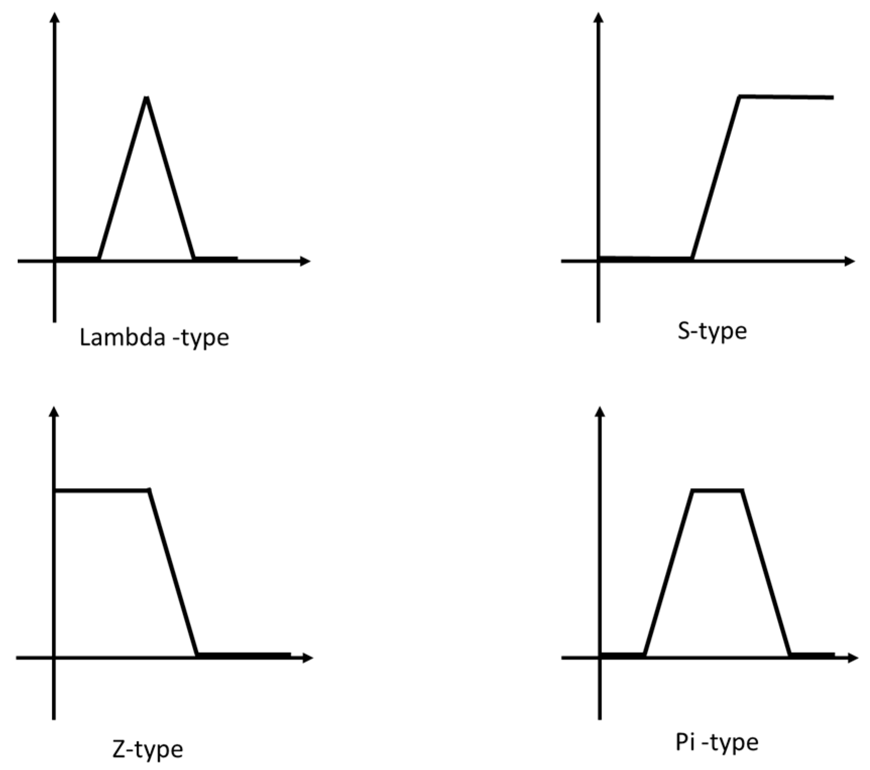
Mendel [40] mentioned that the membership function will be different according to each person’s feelings and judgments, so the given function of the membership is due to people. Most studies have only used standardized membership functions in practical applications. Figure 1 shows four common membership functions: Lambda-type, S-type, Z-type and Pi-type.

The earliest fuzzy reliability was proposed by Cai, Wen and Zhang [41]. The main research focused on the reliability of evaluating the binary-state of each component. However, binary-state fuzzy reliability cannot accurately represent the state in some practical and complex systems such as network systems, power systems, manufacturing operating systems and so forth.

In order to deal with more complex systems, scholars have developed multi-state fuzzy reliability based on the basis of binary-state fuzzy reliability [42]. Multi-state fuzzy reliability divides the interval [0,1] into several subintervals and defines fuzzy sets for each degree of interval state, most of which are defined by expert experience. In order to make up for the lack of expert ability, the latter is combined with fuzzy logic and inference [43], constructing a fuzzy system [44] that can adjust parameters according to various states, strengthen their learning ability and have a better interpretation of more complex systems.

Fuzzy theory pays attention to the essence of the problem and proposes different thinking logics from traditional mathematical theory. Instead, it can obtain significant effects with traditional mathematics. As such, fuzzy applications will next become more specialized. In addition to being able to be applied to reliability such as image recognition [45], mathematical programming [46], algorithms [47] and data exploration [48] and so forth, we can see the traces of fuzzy theory and also prove it. It can also prove the success and breakthrough point of fuzzy theory.

2.3. Time Window

The time window can represent the customer’s demand for time or the service period that the servicer can order or provide. For example, the time window of mass transit indicates that the user can take or pass during certain time periods, the time when the logistics industry is scheduled to deliver the goods, the delivery limit in the production line problem and the dial a ride problem and so forth. Time windows can be applied to these problems by using the characteristics of the time window (density, position, width) to explore the results under different conditions.

When solving the Traveling Salesman Problem, Baker [29] first proposed the concept of time window constraints by establishing the earliest start service time (lower limit of time window) and end service time (upper limit of time window) conditions in each network node. Solomon [30] introduced the time window into the vehicle routing problem (VRP) and used the time window to express the range of service times the customer wanted. Chen and Lee [49] presented two additional models with penalty delays when studying parallel machine scheduling. The first type set the task expiration date to a specific range. When the task was completed on time, there was no additional cost. The second type of model set the expiration date as an interval and the lower and upper limit of the time window were the earliest expiration date and the latest expiration date. As long as the task completion time fell within this interval, there were no additional costs. The second type of model is more reasonable and closer to reality and is more widely used in practical problems.

Solomon and Desrosiers [50] proposed a variety of time window concepts when studying scheduling problems and divided the time window constraints into two categories according to the degree of elasticity: the soft time window and hard time window. The main difference is that the hard time window must fall completely within the set time window. Otherwise, the soft time window is allowed to fall outside the time window but it must be punished. The two are mixed into a comprehensive time window. Figure 2 shows the three time window types, where the X-axis is time, the Y-coordinate indicates the cost of substituting the P function and e and ι represent the lower bound and the upper bound of the time window, respectively.

3. Research Methods and Mathematical Models

This section explains in detail the network model construction process to solve the real problem of traffic network and explores how to meet the various needs of users, obtain the minimum feasible solution and calculate the overall network reliability. Section 3.1 introduces the theorem and lemma of establishing a fuzzy traffic service network and presents the problem solving method and formula deduction. Additionally, for the basic assumptions, please refer to

Table A1. Summary table of the assumptions.

Entry	Assumption
1.	Users must be transported from the source node s to the sink node t
2.	Meet the law of conservation of flow
3.	Each node is absolutely reliable
4.	The capacity of the arcs does not affect each other and is independent of each other
5.	The capacity on each arc is random and given a corresponding probability assignment
6.	The state of the arc can be defined by the fuzzy function

for a summary of the assumptions (see Appendix A).

3.1. Theorem and Lemma

In the network represented in Figure 3, node 1 represents the source node, node 4 represents the sink node, nodes 2 and 3 represent the transit nodes through which the transport process passes and is taken as an example. A summary table that explains the topics step by step has been provided on

Table A2. Summary table explain topics step by step.

Begin.

STEP 1. Input a network. STEP 2. The basic data of each arc, the fuzzy function of each arc flow and time and the fuzzy function value of each arc reliability are provided. STEP 3. Calculate the amount of each type of user per path (arc) and make the total delivery volume meet the demand of individual users and not greater than the upper limit of the transportable capacity of each path (arc). STEP 4. Find out D = (d1, d2, …, ds)-MP candidate solutions by the feasible transport amount of the various types of users, which is described in Theorem 1, Lemma 1, Lemma 2 and Equation (7), in the path obtained in Step 3. STEP 5. Obtain D-MP solutions using the comparison algorithm to check whether the D-MP candidate solution obtained in Step 4 is a D-MP solution by Corollary 1. STEP 6. Consider the effect of time window on D-MP solution by Theorem 2, Lemma 3 and Equations (9) and (10). STEP 7. Use the fuzzy system to obtain the reliability of each arc as described in the Section 3.1.4. STEP 8. Substituting fuzzy set operations into the principle of displacement to find the network reliability that satisfies the time window by Equation (12). STEP 9. Output RFinal.

End.

in the Appendix A. The arc represents the transport path. The basic data of each arc, the fuzzy function of each arc flow and time and the fuzzy function value of each arc reliability are shown in

Table 1. Basic data of each arc.

Arc	Capacity	Probability rk	Shipping Time λ	αk1	αk2
e1	0	0.01	5	1	1
	1	0.02
	2	0.02
	3	0.95
e2	0	0.01	5	1	1
	1	0.01
	2	0.01
	3	0.97
e3	0	0.01	5	1	1
	1	0.02
	2	0.05
	3	0.92
e4	0	0.01	5	1	1
	1	0.01
	2	0.01
	3	0.97
e5	0	0.01	5	1	1
	1	0.04
	2	0.05
	3	0.9
e6	0	0.01	5	1	1
	1	0.03
	2	0.03
	3	0.92

Note: Assume that the user has two requirements for the transportation network, that is, c = 1, 2, α_k¹ and α_k² represents the weight of demand for the first type of user and the second type of user, respectively.

,

Table 2. Fuzzy function of flow and time for each arc.

	Function Value	b1k	b2k	b3k	b4k	b5k	b6k
Arc
e1		1	3	5	7	9	11
e2		1	3	8	6	8	11
e3		1	3	9	7	9	11
e4		1	2	5	7	9	11
e5		1	3	5	6	9	12
e6		1	4	5	7	9	13

and

Table 3. Fuzzy function value of reliability for each arc.

	Function Value	b7k	b8k	b9k	b10k	b11k
Arc
e1		0	0.25	0.5	0.75	1
e2		0	0.25	0.5	0.75	1
e3		0	0.25	0.5	0.75	1
e4		0	0.25	0.5	0.75	1
e5		0	0.25	0.5	0.75	1
e6		0	0.25	0.5	0.75	1

.

3.1.1. Needs Processing of Various User

User demand for services of more than one type in the same network is set to different demand d_c. We assumed that the user had two requirements for the transportation network (d₁, d₂) = (1, 1).

Theorem 1.

When the vector X = (x₁, x₂, …, x_m) is D = (d₁, d₂, …, d_s)-MP, the following two conditions must be met:

• This vector meets various user needs D = (d₁, d₂, …, d_s).
• Test by the comparison algorithm

Theorem 1 illustrates the problems of multiple demand in this study. The following uses Lemma 1 to explain how to find the demand of various users in each path.

Lemma 1.

The transportation network must meet the demand of various users. Here, Equation (2) is used to indicate that the flow of the source node is equal to the flow of the sink node and is also equal to the demand:

x^c_1,1 = x^c_n,n = d_c, for all c = 1, 2, …, s

(2)

The total number of traffic services of item c on each path cannot exceed the upper limit of the path capacity M_k (max capacity), as shown in Equation (3):

$${\displaystyle \sum _{c=1}^s{\alpha }_k^c{x}_{i,j}^c\le M_k for all i=1,2,\mathrm{\dots },n;j=1,2,\mathrm{\dots },n}$$

(3)

The flow must comply with flow conservation. The sum of the incoming flow of each node to class c must be equal to the sum of the outgoing flow, as shown in Equation (4):

$${\displaystyle \sum _{j=1}^n{x}_{i,j}^c={\displaystyle \sum _{k=1}^n{x}_{k,i}^c, for all x_{i,j}^c,x_{k,i}^c\in E,i}}\ne 1 or n$$

(4)

$${\displaystyle \sum _{i=2}^n{x}_{1,i}^c={\displaystyle \sum _{j=1}^{n-1}{x}_{j,n}^c=d_c,for all x_{1,i}^c,x_{j,n}^c\in E}}$$

(5)

In Equation (2), the sum of the shipments must meet the demand of each user. This model uses x^c_1,1 to indicate the source node to provide the sum of the requirements of the cth user. Equation (3) is an important part of this section, which means that each demand will correspond to different weights. The shipments of each flow multiplied by this flow weight in each path cannot exceed the upper capacity of each path (arc). Equation (4) shows that the sum of the inflows of class c in the ith node is equal to the sum of the outflows. Equation (5) indicates that the flow for the source and sink nodes must be the same and must be equal to the demand.

From Equations (2) to (5), we can find the transportable quantity (X¹, X²,…, X^s) which satisfies the demand of each user (d₁, d₂, …,d_s) and find the D = (d₁, d₂, …,d_s)-MP candidate solution.

Lemma 2.

Equation (6) multiplies the sum of the number of c-class users of each arc by the weight of the c-class in each arc to find the sum of all of the user’s transport amount X on each path (arc) and find the D-MP candidate solution.

$${\displaystyle \sum _{c=1}^s{\alpha }_k^c{x}_{i,j}^c} for all I= 1,2, \dots , n; j= 1,2, \dots , n and x_{i,j}^c=x_k^c$$

(6)

The above equation indicates that the user’s transport amount on each path (arc) cannot exceed the upper limit of the capacity set for each path (arc). In order to facilitate the expression of all solutions, this is denoted by the symbol Ω : Ω ≡ {X | X meet all categories of user demand D = (d₁, d₂, …,d_s)}. In set Ω, when a vector X is smaller than the vector Y and the vector X satisfies all kinds of user requirements d₁, d₂, …, d_s, the vector Y is an infeasible solution and must be eliminated. In simple terms, the D-MP solution must be the smallest and most feasible solution to meet the demand. Here, the set of D-MP solutions is represented by Ω_min and the reliability that satisfies all user requirements d₁, d₂, …, d_s is obtained, which is expressed by Equation (7):

R_{d1, d2, …,ds} = Pr{Ω} = Pr{Y∈Ω | Y ≥ X for a (d₁, d₂, …,d_s) -MP }

(7)

In order to obtain more accurate network reliability, all D-MP solutions must be found in all D-MP candidate solutions. The next section will detail the process and method.

3.1.2. Check the D-MP Candidate Solution

Among all of the D-MP candidate solutions, there may be a non-minimum feasible solution that satisfies the requirements. In the following study, the comparison algorithm was used to check the solutions in the Ω set, these non-minimum feasible solutions were deleted and finally D-MP solutions were obtained. The steps and methods for checking the D-MP candidate solutions are described in detail in Corollary 1.

Corollary 1.

This step uses the comparison algorithm to check the D-MP candidate solution. The following is a detailed description of the calculation procedure of the comparison algorithm:

Step 1:

Set all of the previous D-MP candidate solution sets as P = (X₁, X₂, …, X_o), representing a total of o candidate solutions, then, it is necessary to check whether each D-MP candidate solution is a D-MP solution.

Step 2:

In addition, this study set up another set, I =∅. This set does not have a solution at the beginning, so it is an empty set. This set stores the solution that is found by the comparison algorithm to not satisfy the minimum requirement.

Step 3:

Checking from the first candidate solution X₁, compare with the remaining candidate solutions X₂ to X_o. If the solution is checked, all solutions are greater than or equal to the solutions of the other solution and then placed in set I, otherwise it is the D-MP solution.

Step 4:

After checking the first candidate solution, X₁, X₂ to X_o are sequentially calculated. If the solution to be checked is larger than the remaining one, it will be placed in set I.

Step 5:

After checking the final solution X_o, end the inspection cycle.

3.1.3. Time Window Limit Processing

After the D-MP solution is obtained, this step uses the time window to process the user’s time requirements. This study used the limitation of the hard time window. When the time exceeds the maximum tolerable range of the user, this solution is regarded as an infeasible solution. If someone arrives early, they must wait until the lower limit of the time window to start the next service. The detailed calculation process is explained below.

Theorem 2.

When vector X = (x₁, x₂, …, x_m) is the standard (quasi) D-MP solution, the following two conditions must be met.

• Vector X satisfies the comparison algorithm Test
• Vector X must satisfy the requirement D = (d₁, d₂, …, d_s) before considering the time window.

Lemma 3.

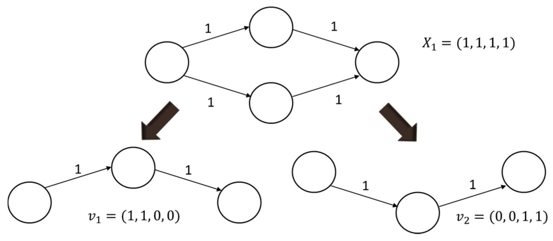
In order to define the time windows of all paths separately, before the time for calculating each solution, all the time window routes in each solution are proposed for calculation and they are arranged in v routes, as shown in Figure 4. In the time window, the time includes the lead time, transit time, process time and arrival time. This study set the process time to C^v_a,b, which means the current accumulated time. Equation (8) is the assumed time of the source node; here we set the starting time as 0.

C^v_1,1 = 0

(8)

In order to clearly indicate the time before and after the time window processing, this study defined two kinds of time: arrival time A and process time C. Equation (9) represents the arrival time that has not been processed by the time window and Equation (10) represents the process time after this time window has been processed.

A^v_a,b = C^v_(a−1),a + Ft ( w_a,b x_a,b +λ_a,b), for 0 ≤ a ≤ n, 0 ≤ b ≤ n, v = 1, 2,…, w

(9)

$$C_{a,b}^v =\{\begin{array}{ll}{A}_{a,b}^v& if e_{t^b}\le A_{a,b}^v\le l_{t^b}\\ e_{t^b}& if A_{a,b}^v<e_{t^b}\\ not exist& otherwise\end{array}$$

(10)

Below is a detailed description of the processing of the time window. Equation (9) is the arrival time from the a node to the next node b in the vth route. This step is the previous site process time C^v_(a−1),a plus the time before the flow into the node (w_a,b x_a,b) plus the transit time λ_a,b. Due to the limitation of applying the hard time window, in the early arrival, one must wait until the lower limit of the time window to move to the next step, which means that arrival time A does not necessarily equal the next departure time. Equation (10) performs the subsequent processing for arrival time A: when the arrival time is within the time window $e_{t^b}\le A_{a,b}^v\le l_{t^b}$, then arrival time A is equal to the departure time C^v_a,b = A^v_a,b; if the arrival time A is earlier than the lower limit of the time window $A_{a,b}^v<e_{t^b}$, one must wait until the lower limit of the time window $e_{t^b}$ for the next step of service processing; if the time exceeds the upper limit of the time window $l_{t^b}$, this solution will be considered as an infeasible solution. Figure 5 is a graph of the time relationships of the time windows.

This study used the concept of fuzzy theory to define each path fuzzy set, indicating the state of the path under different flow and time. Finally, the fuzzy system was used to derive the reliability. Lemma 4 will be explained in detail.

Lemma 4.

After finding the D-MP solution, the user can use the function value in the past data to establish a membership function to define each path state. Next, fuzzy inference, fuzzy rule base and defuzzification are used to establish the fuzzy system and the reliability of each arc is calculated.

3.1.4. Fuzzy System Construction

This step uses the fuzzy function to process the previous section to obtain the flow of each arc. First, we had to define the input and output variables. In addition to the flow fuzzy function as the fuzzy system input variable, we took the transit time Ft of each arc as another input variable and finally used the reliability function as the output variable. This model had a two-input and single-output control system architecture and used Z-type incremental fuzzy function (Z function), triangular fuzzy function (triangular function) and Z-type decreasing fuzzy number (S function) to represent low, medium and high states. Figure 6, Figure 7 and Figure 8 are fuzzy function definition diagrams for input and output.

The next step is to establish the fuzzy rule base. The main purpose of the fuzzy rule base is to define the relationship between the output and input. Here, the rule library was used to express the relationship between time, flow and reliability as the basis for subsequent inference.

Table 4. Example of fuzzy rule library.

Reliability		Time
		Short	Normal	Long
Flow	Low	Very High	High	High
	Normal	High	Normal	Low
	High	High	Low	Very Low

is used here to represent this example of rule library architecture.

The next part is fuzzy inference, using the rules derived from experience or related knowledge, in the form of the premise (If) and the conclusion (Then), which are divided into the premise (If), the conclusion (Then) and the integration operation. We used the minimum inference method and Figure 9 shows the inference mode representation for this method.

As the center of area method is a well-known and continuously adopted method of research [51,52], we used it to conduct the defuzzification step and to defuzzify the value of the previous step into the value of the problem. The center of area method is a weighted average calculation method. In the center of area method, we used the continuous integral type of the center of area method. Suppose that the domain of the output attribution function C falls between the intervals a to b, the model is as shown in Equation (11).

$$y=\frac{{\displaystyle {\int }_a^{b}C(y)ydy}}{{\displaystyle {\int }_a^{b}C(y)dy}}$$

(11)

After knowing the reliability of each arc, we finally applied the fuzzy intersection arithmetic formula (t-norm class) to the displacement principle to calculate the network reliability. Equation (12) is a mathematical expression representing fuzzy network reliability.

R_Final = u_R^k(X) = t(u_R¹(x₁), u_R²(x₂),…, u_R^k(x_k) )

(12)

4. Experiments

Section 4 introduces how the study solved two practical problems: a single-time window and single service network and a multi-time window and multi-service network. The above actual situation was to explore practical issues such as traffic impact path reliability and time window limits.

4.1. Single-Time Window and Single Service Network

Here, we discuss the first real situation: a single-time window and single service network. This issue explores the network from a user perspective. After the user decides to use a single service, in addition to the overall network reliability, the user will want to know which route arrives at the sink node and has a high degree of reliability among the many routes to the destination. The network model is shown in Figure 10. This network diagram has a source node, a sink node and four paths (arcs). The user demand is D = 3.

Table 5. Basic information of each arc.

Arc	Capacity	Reliability	Operation Lead Time/Unit Passenger	Transit Time	αk1
e1	0	0.01	2	4	1
	1	0.02
	2	0.02
	3	0.95
e2	0	0.01	3	4	1
	1	0.01
	2	0.005
	3	0.005
	4	0.97
e3	0	0.01	2	3	1
	1	0.05
	2	0.06
	3	0.88
e4	0	0.01	3	5	1
	1	0.02
	2	0.03
	3	0.94

shows the upper limit of the transportable capacity of each arc and the corresponding probability value, operation lead time, transit time and commodity ratio. This study developed the fuzzy sets as shown in

Table 6. Fuzzy function value of flow and time for each arc.

	Function Value	b1k	b2k	b3k	b4k	b5k	b6k
Arc
e1		1	1.5	3	9	11	13
e2		1	1.5	3	9	11	13
e3		0.5	1	3	9	11	13
e4		0.5	1	3	9	11	13

(fuzzy function value of flow and time for each arc) and

Table 7. Fuzzy function value of reliability for each arc.

	Function Value	b7k	b8k	b9k	b10k	b11k
Arc
e1		0	0.25	0.5	0.75	1
e2		0	0.25	0.5	0.75	1
e3		0	0.25	0.5	0.75	1
e4		0	0.25	0.5	0.75	1

(fuzzy function value of reliability for each arc) according to the rule based on the description in Section 2.2. In order to deal with more complex systems, scholars have developed multi-state fuzzy reliability based on the basis of binary-state fuzzy reliability [42]. Multi-state fuzzy reliability divides the interval [0,1] into several subintervals and defines fuzzy sets for each degree of interval state, most of which are defined by expert experience. In order to make up for the lack of expert ability, the latter is combined with fuzzy logic and inference [43], constructing a fuzzy system [44], which can adjust parameters according to various states, strengthen their learning ability and have a better interpretation of more complex systems.

Step 1. The amount of transport on each path must not exceed the upper limit of transport (M₁, M₂, M₃, M₄) = (3, 4, 3, 3) for each path (arc). For the convenience of representation, let X = (x_1,2, x_2,4, x_1,3, x_3,4) = (x₁¹, x₂¹, x₃¹, x₄¹).

0 ≤ x₁¹ ≤ 3

(13)

0 ≤ x₂¹ ≤ 4

(14)

0 ≤ x₃¹ ≤ 3

(15)

0 ≤ x₄¹ ≤ 3

(16)

This network must meet customer demand D = 3:

x₁¹ + x₃¹ = 3

(17)

x₂¹ + x₄¹ = 3

(18)

According to the flow conservation theory, the sum of the inflow and outflow of node 2 and node 3 must be the same:

x₁¹ = x₂¹

(19)

x₃¹ = x₄¹

(20)

Find all feasible solutions X¹ = (x₁¹, x₂¹, x₃¹, x₄¹) by the exhaustive method (as shown in

Table 8. The process of the exhaustive method.

0 ≤ x11 ≤ 3	0 ≤ x21 ≤ 4	0 ≤ x31 ≤ 3	0 ≤ x41 ≤ 3
0	0	0	0
1	0	0	0
0	1	0	0
0	0	1	0
0	0	0	1
:	:	:	:
:	:	:	:
:	:	:	:
:	:	:	:
:	:	:	:
3	3	3	3

) through Equations (13)–(20). This process is shown in Table 8:

Through the exhaustive process, we can obtain the results of the feasible solution, as shown in

Table 9. The results of the feasible solution.

Feasible Delivery Method of Group I	Service	x11	x21	x31	x41
1	X1	3	3	0	0
2	X2	0	0	3	3
3	X3	2	2	1	1
4	X4	1	1	2	2

:

Step 2. Find all possible D-MP candidate solutions from the feasible transport mode X obtained in Step 1.

$$\{\begin{array}{l}{x}_1=x_1^1\\ x_2=x_2^1\\ x_3=x_3^1\\ x_4=x_4^1\end{array}$$

We bring in Equation (6) to find the D-MP candidate solution: X₁ = (3, 3, 0, 0), X₂ = (0, 0, 3, 3), X₃ = (2, 2, 1, 1) and X₄ = (1, 1, 2, 2).

Step 3. This step uses the comparison algorithm to check whether the D-MP candidate solution obtained in Step 2 is a real D-MP solution. The final test results are shown in

Table 10. The results of Step 3.

Tested X	Whether It Is a D-MP Solution
X1 = (3, 3, 0, 0)	Yes
X2 = (0, 0, 3, 3)	Yes
X3 = (2, 2, 1, 1)	Yes
X4 = (1, 1, 2, 2)	Yes

.

Step 4. In the actual transportation service network, not only must the user successfully reach the sink node but must also arrive under the users’ condition of time, so the time limit must be considered. This step uses the time window as a time limit, where the upper limit of the time window represents the user’s tolerance for a delayed arrival. When the time is exceeded, the solution is an infeasible solution. The lower limit of the time window represents the time at which the estimated service start time. If it arrives early, it must wait until the node’s departure time to continue moving.

Here, we assumed that the time window of the sink node (node 4) was {$e_{t^4}$,$l_{t^4}$} = {0, 25} (the sink node was the last stop, so there was no lower limit). In order to facilitate the expression and calculation time, we listed the D-MP solutions processed by the comparison algorithm in

Table 11. The results of Step 3.

D-MP	Processing Route	The Time of Source Node for This MP	Time Window of this MP
X1	{e1, e2}	C11,1 = 0	{$e_{t^4}$,$l_{t^4}$} = {0, 25}
X2	{e3, e4}	C21,1 = 0	{$e_{t^4}$,$l_{t^4}$} = {0, 25}
X3	{e1, e2}, {e3, e4}	C31,1 = 0, C41,1 = 0	{$e_{t^4}$,$l_{t^4}$} = {0, 25}
X4	{e1, e2}, {e3, e4}	C51,1 = 0, C61,1 = 0	{$e_{t^4}$,$l_{t^4}$} = {0, 25}

.

Check X₁ = (3, 3, 0, 0) as an example:

This D-MP solution only has the {e₁, e₂} route, so only this route needed to be checked. The following is the detailed flow of the calculation:

At the start time of node 1, C¹_1,1 = 0 and the arrival time of the second station (node 2) is calculated as A¹_1,2:

A¹_1,2 = C¹_1,1 + Ft(w_1,2 x_1,2+λ_1,2 ) = 0 + 2 × 3 + 4 =10

(21)

After calculating the arrival time, the next step is to calculate the process time after the time window processing C¹_1,2. However, node 2 does not assume a time window, so C¹_1,2 = A¹_1,2 = 10.

The flow time at node 2 is C¹_1,2 = 10, then the arrival time A¹_2,3 of the third station (node 4) is calculated:

A¹_2,3 = C¹_1,2 + Ft(w_2,3 x_2,3+λ_2,3 ) = 10 + 3 × 3 + 4 = 26

(22)

After calculating the arrival time, the next step is to calculate the process time C¹_2,4 after the time window processing:

$$C_{1,3}^1=\{\begin{array}{ll}{A}_{2,3}^1& if 0\le A_{2,3}^1\le 25\\ 0& if A_{2,3}^1<0\\ not exist& otherwise\end{array}$$

(23)

Substituting A¹_2,4 = 26, we found that the process time exceeded the upper limit of the time window of 25, so was unable to complete the service in time, which means that this solution is an infeasible solution under the consideration of the time window conditions.

Finally, the results are shown in

Table 12. The results of Step 4.

	Whether to Meet the Time Window Limit
X1	No
X2	Yes
X3	Yes
X4	Yes

.

Step 5. In the actual traffic service network, the path state will affect the reliability. In this step, the reliability of each arc is obtained by means of a fuzzy system. First, we established a fuzzy rule base and fuzzy set for each flow, time and reliability.

Table 13. Fuzzy rule library.

Reliability		Time
		Short	Normal	Long
Flow	Low	Very High	High	High
	Normal	High	Normal	Low
	High	High	Low	Very Low

presents the sample fuzzy rule library and

Table 14. Transport time and flow for each arc.

	x1		x2		x3		x4
	Flow	Time	Flow	Time	Flow	Time	Flow	Time
X2	0	0	0	0	3	10	3	11
X3	2	8	2	10	1	6	1	8
X4	1	6	1	7	2	7	2	11

shows the time and flow of each path in each set of solutions.

In this study, the reliability of each arc was determined by the fuzzy system constructed.

Table 15. Fuzzy reliability of each arc.

	x1	x2	x3	x4
X2	0.92	0.92	0.25	0.25
X3	0.558	0.529	0.92	0.92
X4	0.92	0.92	0.558	0.409

shows the reliability results calculated using the fuzzy system.

Step 6. First, find the reliability of each D-MP solution, as shown in Equations (24)–(26):

X₂ = 1 × 1 × 0.25 × 0.25 = 0.0625

(24)

X₃ = 0.558 × 0.529 × 0.92 × 0.92 = 0.2498

(25)

X₄ = 0.92 × 0.92 × 0.558 × 0.409 = 0.1932

(26)

We used fuzzy intersection calculations to satisfy customer demand and time windows and finally obtained the overall network reliability by using the algebraic intersection formula to calculate:

Rfinal = Pr{X2∪X3∪X4 }

= [Pr{X2} + Pr{X3} + Pr{X4}] − [Pr{X2⋂X3} + Pr{X2⋂ X4} + Pr{X3⋂ X4}] + [Pr{ X2⋂ X3⋂ X4}]

= [Pr{X2} + Pr{X3} + Pr{X4}] − [t(X2,X3) + t(X2,X4) + t(X3,X4)] + t(X2,X3,X4)

= 0.0625 + 0.2498 + 0.1932 − (0.0625 × 0.2498 + 0.0625 × 0.1932 + 0.2498 × 0.1932) +

(0.0625 × 0.2498 × 0.1932)

= 0.4326

Considering the fuzzy state and time window constraints, the network had a 43.26% reliability of meeting the user demand.

4.2. Multi-Time Window and Multi-Service Network

We also present a second reality of a multi-time window and multi-service network. This issue explores the network from a server perspective. In a complex network, there is more than one demand, source node and sink node. The network model is shown in Figure 11, which has two source nodes, two sink nodes and eight paths (arcs). The first sink node (node 7) has two service requirements (d1, d2) = (1, 2); and the second sink node (node 8) has two service requirements (d1, d2) = (2, 1).

Table 16. Basic information of each arc.

Arc	Capacity	Reliability	Operation Lead Time/Unit Passenger	Transit Time	αk1	αk2
e1	0	0.02	1	4	1	1
	1	0.02
	2	0.03
	4	0.93
e2	0	0.01	1.5	4	1	1
	1	0.02
	2	0.02
	3	0.95
e3	0	0.01	1	3	1	2
	1	0.04
	2	0.06
	3	0.89
e4	0	0.01	2	5	1	1
	1	0.01
	2	0.01
	3	0.01
	4	0.96
e5	0	0.01	2	6	1	1
	1	0.01
	2	0.02
	3	0.01
	4	0.95
e6	0	0.05	1	3	1	2
	1	0.05
	2	0.05
	3	0.85
e7	0	0.01	1	3	1	1
	1	0.03
	2	0.06
	3	0.9
e8	0	0.01	1.5	4	1	1
	1	0.02
	2	0.02
	3	0.02
	4	0.94

shows the upper limit of the transportable capacity of each arc and the corresponding probability value, operation lead time, transit time and commodity ratio. This study developed the fuzzy sets as shown in

Table 17. Fuzzy function values of flow and time for each arc.

	Function Value	b1k	b2k	b3k	b4k	b5k	b6k
Arc
e1		1	1.5	3	9	11	13
e2		1	1.5	3	9	11	13
e3		0.5	1	3	9	11	13
e4		0.5	1	3	9	11	15
e5		1	1.5	3	9	11	15
e6		1	1.5	3	9	11	13
e7		0.5	1	3	9	11	13
e8		0.5	1	3	9	11	13

(the fuzzy function values of flow and time for each arc) and

Table 18. Fuzzy function values of reliability for each arc.

	Function Value	b7k	b8k	b9k	b10k	b11k
Arc
e1		0	0.25	0.5	0.75	1
e2		0	0.25	0.5	0.75	1
e3		0	0.25	0.5	0.75	1
e4		0	0.25	0.5	0.75	1
e5		0	0.25	0.5	0.75	1
e6		0	0.25	0.5	0.75	1
e7		0	0.25	0.5	0.75	1
e8		0	0.25	0.5	0.75	1

(the fuzzy function values of reliability for each arc), according to the rule based on the description in Section 2.2. In order to deal with more complex systems, scholars have developed multi-state fuzzy reliability based on the basis of binary-state fuzzy reliability [42]. Multi-state fuzzy reliability divides the interval [0,1] into several subintervals and defines fuzzy sets for each degree of interval state, most of which are defined by expert experience. In order to make up for the lack of expert ability, later combined with fuzzy logic and inference [43], constructing a fuzzy system [44], can adjust parameters according to various states, strengthen their learning ability and have a better interpretation of more complex systems.

Step 1. The amount of transport on each path must not exceed the upper limit of transport (M₁, M₂, M₃, M₄, M₅, M₆, M₇, M₈) = (3, 3, 3, 4, 4, 3, 3, 3) for each path (arc). For the convenience of representation, let X = (x_1,3, x_2,4, x_3,5, x_3,6, x_4,5, x_4,6, x_5,7, x_6,8) = (x₁, x₂, x₃, x₄, x₅, x₆, x₇, x₈).

0 ≤ x₁¹ + x₁² ≤ 3

(27)

0 ≤ x₂¹ + x₂² ≤ 3

(28)

0 ≤ x₃¹ + x₃² ≤ 3

(29)

0 ≤ x₄¹ + x₄² ≤ 3

(30)

0 ≤ x₅¹ + x₅² ≤ 3

(31)

0 ≤ x₆¹ + x₆² ≤ 3

(32)

0 ≤ x₇¹ + x₇² ≤ 3

(33)

0 ≤ x₈¹ + x₈² ≤ 3

(34)

This network must meet the customer demand of the first sink node (Node 7) (d₁, d₂) = (1, 2) and the second sink node (Node 8) (d₁, d₂) = (2, 1):

x₃¹ + x₅¹ = 1

(35)

x₅² + x₇² = 2

(36)

x₄¹ + x₆¹ = 2

(37)

x₄² + x₆² = 1

(38)

According to the flow conservation theory, the sum of the inflow and outflow of nodes 3–6 must be the same:

x₁¹ + x₁² = x₃¹ + x₃² + x₄¹ + x₄²

(39)

x₂¹ + x₂² = x₅¹ + x₅² + x₆¹ + x₆²

(40)

x₃¹ + x₃² + x₅¹ + x₅² = x₇¹ + x₇²

(41)

x₄¹ + x₄² + x₆¹ + x₆² = x₈¹ + x₈²

(42)

This process is shown in

Table 19. The process of the exhaustive method.

$0\le {\mathit{x}}_1^1\le 4$	$0\le {\mathit{x}}_2^1\le 4$	$0\le {\mathit{x}}_3^1\le 3$	$0\le {\mathit{x}}_4^1\le 4$	$0\le {\mathit{x}}_5^1\le 4$	$0\le {\mathit{x}}_6^1\le 3$	$0\le {\mathit{x}}_7^1\le 3$	$0\le {\mathit{x}}_8^1\le 3$	$0\le {\mathit{x}}_1^2\le 4$	$0\le {\mathit{x}}_2^2\le 4$	$0\le {\mathit{x}}_3^2\le 3$	$0\le {\mathit{x}}_4^2\le 4$	$0\le {\mathit{x}}_5^2\le 4$	$0\le {\mathit{x}}_6^2\le 3$	$0\le {\mathit{x}}_7^2\le 3$	$0\le {\mathit{x}}_8^2\le 3$
0	0	0	0	0	0	0	0	0	0	0	0	0	0	0	0
0	0	0	0	0	0	0	0	0	0	0	0	0	0	1	0
0	0	0	0	0	0	0	0	0	0	0	0	0	1	0	0
:	:	:	:	:	:	:	:	:	:	:	:	:	:	:	:
:	:	:	:	:	:	:	:	:	:	:	:	:	:	:	:
:	:	:	:	:	:	:	:	:	:	:	:	:	:	:	:
4	4	3	4	4	3	3	3	4	4	3	4	4	3	3	3

to find all feasible solutions X¹ = (x₁¹, x₂¹, x₃¹, x₄¹, x₅¹, x₆¹, x₇¹, x₈¹) and X² = (x₁², x₂², x₃², x₄², x₅², x₆², x₇², x₈²) by the exhaustive method (as shown in

Table 20. Feasible solutions.

Feasible Solutions	Service	x1c	x2c	x3c	x4c	x5c	x6c	x7c	x8c
1	x11	1	2	0	1	1	1	1	2
	x12	2	1	1	1	1	0	2	1
2	x21	2	1	1	1	0	1	1	2
	x22	1	2	1	0	1	1	2	1
3	x31	2	1	1	1	0	1	1	2
	x32	1	2	0	1	1	1	2	1
4	x41	2	1	0	2	1	0	1	2
	x42	1	2	1	0	1	1	2	1
5	x51	2	1	0	2	1	0	1	2
	x52	1	2	0	1	1	1	2	1
6	x61	3	0	1	2	0	0	1	2
	x62	0	3	0	0	2	1	2	1

) through Equations (27)–(42):

Step 2. Find all possible D-MP candidate solutions from the feasible transport mode X obtained in step 1.

x₁ = x₁¹ + x₁²

x₂ = x₂¹ + x₂²

x₃ = x₃¹ +2 x₃²

x₄ = x₄¹ + x₄²

x₅ = x₅¹ + x₅²

x₆ = x₆¹ +2 x₆²

x₇ = x₇¹ + x₇²

x₈ = x₈¹ + x₈²

We found the D-MP candidate solution: (3, 3, 2, 2, 2, 2, 3, 3), (3, 3, 3, 1, 1, 2, 3, 3), (3, 3, 1, 3, 1, 3, 3, 3), (3, 3, 2, 2, 2, 2, 3, 3), (3, 3, 0, 3, 2, 2, 3, 3), (3, 3, 2, 2, 2, 2, 3, 3). Among them, it was found that there were duplicate solutions and after deletion, the solution was solved as X₁ = (3, 3, 2, 2, 2, 2, 3, 3), X₂ = (3, 3, 3, 1, 1, 2, 3, 3), X₃ = (3, 3, 1, 3, 1, 3, 3, 3) and X₄ = (3, 3, 0, 3, 2, 2, 3, 3).

Step 3. This step uses the comparison algorithm to check whether the D-MP candidate solution obtained in Step 2 is a real D-MP solution. The final test results are shown in

Table 21. The results of Step 3.

Tested X	Whether It Is a D-MP Solution
X1= (3, 3, 2, 2, 2, 2, 3, 3)	Yes
X2= (3, 3, 3, 1, 1, 2, 3, 3)	Yes
X3= (3, 3, 1, 3, 1, 3, 3, 3)	Yes
X4 = (3, 3, 0, 3, 2, 2, 3, 3)	Yes

.

Next, the user’s time limit is processed and a fuzzy system is established to determine the reliability of each path and finally the overall network reliability is obtained.

Step 4. This step establishes multiple time windows on multiple nodes as a constraint on the network model, where the upper limit of the time window represents the user’s tolerance for a delayed arrival. When the time is exceeded, the solution is an infeasible solution. The lower limit of the time window represents the time at which the estimated service start time. If it arrives early, it must wait until the node’s departure time to continue moving. In order to facilitate the expression and calculation time, we list the D-MP solutions processed by the comparison algorithm, as shown in

Table 22. The test results of Step 4.

D-MP	Split Path	Starting Time
X1	{e1, e3, e7},{e2, e5, e7},{e1, e4, e8},{e2, e6, e8}	0
X2	{e1, e3, e7},{e2, e5, e7},{e1, e4, e8},{e2, e6, e8}	0
X3	{e1, e3, e7},{e2, e5, e7},{e1, e4, e8},{e2, e6, e8}	0
X4	{e2, e5, e7},{e1, e4, e8},{e2, e6, e8}	0

.

Before the calculation, we proposed the D-MP solution as four routes of {e₁, e₃, e₇}, {e₂, e₅, e₇}, {e₁, e₄, e₈} and {e₂, e₆, e₈}. Here we use X₁ = (3, 3, 2, 2, 2, 2, 3, 3) as an example to directly use

Table 23. Time window inspection process of X_1.

	Node & Time Window		Node & Time Window		Node & Time Window
	Arrival Time	Process Time	Arrival Time	Process Time	Arrival Time	Process Time
{e1, e3, e7} = {3, 2, 3}	Node 3, {6, 9}		Node 5, no set		Node 7, {0, 23}
	0 + 1 × 3 + 4	7	7 + 1 × 2 + 3	12	12 + 1 × 3 + 3	18 (O)
{e2, e5, e7} = {3, 2, 3}	Node 4, {6, 9}		Node 5, no set		Node 7, {0, 23}
	0 + 1.5 × 3 + 4	8.5	8.5 + 2 × 2 + 6	18.5	18.5 + 1 × 3 + 3	24.5 (X)
{e1, e4, e8} = {3, 2, 3}	Node 3, {6, 9}		Node 6, no set		Node 8, {0, 27}
	0 + 1 × 3 + 4	7	7 + 2 × 2 + 5	16	16 + 1.5 × 3 + 4	24.5 (O)
{e2, e6, e8} = {3, 2, 3}	Node 4, {6, 9}		Node 6, no set		Node 8, {0, 23}
	0 + 1.5 × 3 + 4	8.5	8.5 + 1 × 2 + 3	13.5	13.5 + 1.5 × 3 + 4	22 (O)

to express the detailed process of checking the solution.

The arrival time is as Equation (43):

A^v_a,b = C^v_(a−1),a + Ft(w_a,b x_a,b +λ_a,b), for 0 ≤ a ≤ n, 0 ≤ b ≤ n, v = 1, 2,…, w

(43)

The process time is as Equation (44):

$$C_{a,b}^v =\{\begin{array}{ll}{A}_{a,b}^v& if e_{t^b}\le A_{a,b}^v\le l_{t^b}\\ e_{t^b}& if A_{a,b}^v<e_{t^b}\\ not exist& otherwise\end{array}$$

(44)

Table 24. The results of Step 4.

D-MP Solutions	Whether to Meet the Time Window Limit
X1	No
X2	Yes
X3	Yes
X4	Yes

shows the time window test D-MP solution results in Step 4.

Step 5. In this step, the reliability of each arc is obtained by means of a fuzzy system. First, establish a fuzzy rule base and fuzzy set for each flow, time and reliability.

Table 25. Fuzzy rule library.

Reliability		Time
		Short	Normal	Long
Flow	Low	Very High	High	High
	Normal	High	Normal	Low
	High	High	Low	Very Low

presents the sample fuzzy rule library and

Table 26. Transport time and flow for each arc.

X2	x1		x2		x3		x4
	flow	time	flow	time	flow	time	flow	time
	3	7	3	8.5	3	6	1	7
	x5		x6		x7		x8
	flow	time	flow	time	flow	time	flow	time
	1	8	2	5	3	6	3	8.5
X3	x1		x2		x3		x4
	flow	time	flow	time	flow	time	flow	time
	3	7	3	8.5	1	4	3	11
	x5		x6		x7		x8
	flow	time	flow	time	flow	time	flow	time
	1	8	3	6	3	6	3	8.5

shows the time and flow of each path in each set of solutions.

In this study, the reliability of each arc was determined by the fuzzy system constructed. The reliability calculation results of each path in are shown in

Table 27. Fuzzy reliability of each arc.

X2	x1	x2	x3	x4
	0.25	0.25	0.25	0.75
	x5	x6	x7	x8
	0.92	0.558	0.25	0.25
X3	x1	x2	x3	x4
	0.25	0.25	0.75	0.191
	x5	x6	x7	x8
	0.92	0.25	0.25	0.25

.

Step 6. First, find the reliability of each D-MP solution, as shown in Equations (45) and (46):

X₂ = 0.25 × 0.25 × 0.25 × 0.75 × 0.92 × 0.558 × 0.25 × 0.25

(45)

X₃ = 0.25 × 0.25 × 0.75 × 0.191 × 0.92 × 0.25 × 0.25 × 0.25

(46)

The final result was X₂ = 0.000376, X₃ = 0.000129

We used fuzzy intersection calculations to satisfy customer demand and time windows and finally obtained the overall network reliability by using the Algebraic intersection formula to calculate:

Rfinal = Pr{X2∪X3}

= [Pr{X2}+Pr{X3} − [Pr{X2⋂ X3}

= Pr{X2}+Pr{X3}− t(X2,X3)

= 0.000376 + 0.000129 − 0.000376 · 0.000129

= 0.000504

Considering the fuzzy state and the time window, this network can hardly meet all of the user demand. Compared with the first example, this example has more paths belonging to the high traffic and high load state. For the definition of time fuzzification, most of them were long-term states and more time window limits were set up. The above two points suggest that users have more and higher requirements on the service. Therefore, the network cannot meet the demand of users and it is necessary to discover the crux of the problem for immediate improvements.

5. Conclusions

This study used the two focuses of time window and fuzzy theory to improve the traditional reliability network regarding the lack of expression of the time and reliability of the traffic service network. In the past, with a traditional network, the time limit was often only limited to the overall time, and the processing time was not delicate enough as in the actual traffic service network, so the user will experience a different duration because of the route length. Due to different perceptions in time, during the construction of the network model, it is necessary to set different time limits for different routes. The hard time window characteristics only matched the characteristics of the transportation service network—there will not be an early outbound time from the station due to early pit stops and the vehicles entering the station early must wait until the scheduled outbound time to depart. In addition to the conditions for setting up time at the sink node, it may be necessary to set time limits on some sites such as the transfer node. The above can use the time window to express the characteristics of the network. On the assumption of reliability, in traditional networks, the reliability of each arc is assumed at the beginning, but this study considered there would be different reliabilities due to the different conditions of the arc. For example, when a road is in a traffic jam state, accidents are more likely to occur, and reliability is reduced. Therefore, this study used fuzzy theory to define a set of states with different arcs, so that the arc would have different reliabilities due to different current flows.

Based on the above improvements to the traditional network, our network model could fully express the real network used in real-world networks about traffic or in networks that require more detail on time, as reliability can change due to different state changes. These networks can be applied to this research model. After comparing two different examples, we finally found that because several paths of the network were in a high load state, this resulted in a significant decline in overall network reliability.

The main issues discussed in this study were fuzzy theory and network reliability and these have increased the limitations of many realities. The current research results will be used to establish a prototype and successfully solve the real problem. This paper has some limitations, which will be strengthened in future research. First, more factors will be considered to strengthen the transportation network to be more in line with the real situation; for example, by considering which path or under what demand there will be poor network performance to improve these symptoms and improve the critical path to increase the reliability of the network. Moreover, in the fuzzy function hypothesis, we used the general triangular fuzzy function and the Z function to define the flow, time and reliability and then established the reliability of each path by the fuzzy law library inference. We can further study and analyze past data and transform them into fuzzy functions of each state to establish a fuzzy rule base, which will more accurately infer the reliability of reality and effectively provide a more complete model as a reference for future improvement.

References

- Papakammenos, D.J.; Dialynas, E.N. Reliability and cost assessment of power transmission networks in the competitive electrical energy market. IEEE Trans. Power Syst. 2004, 19, 390–398. [Google Scholar] [CrossRef]
- Dhillon, B.S. Transportation Systems Reliability and Safety; CRC Press: Boca Raton, FL, USA, 2016. [Google Scholar]
- Lin, Y.K. Performance evaluation for the logistics system in case that capacity weight varies from arcs and types of commodity. Int. J. Prod. Econ. 2007, 107, 572–580. [Google Scholar] [CrossRef]
- Yeh, W.C.; Lin, J.S. New parallel swarm algorithm for smart sensor systems redundancy allocation problems in the Internet of Things. J. Supercomput. 2018, 74, 4358–4384. [Google Scholar] [CrossRef]
- Grout, J.R. Influencing a Supplier Using Delivery Windows: Its Effect on the Variance of Flow Time and On-Time Delivery. Decis. Sci. 1998, 29, 747–764. [Google Scholar] [CrossRef]
- Zhang, J.; Lam, W.H.; Chen, B.Y. On-time delivery probabilistic models for the vehicle routing problem with stochastic demands and time windows. Eur. J. Oper. Res. 2016, 249, 144–154. [Google Scholar] [CrossRef]
- Shen, Y. A new simple algorithm for enumerating all minimal paths and cuts of a graph. Microelectron. Reliab. 1995, 35, 973–976. [Google Scholar] [CrossRef]
- Yeh, W.C. A simple heuristic algorithm for generating all minimal paths. IEEE Trans. Reliab. 2007, 56, 488–494. [Google Scholar] [CrossRef]
- Yeh, W.C. Search for all MCs in networks with unreliable nodes and arcs. Reliab. Eng. Syst. Saf. 2003, 79, 95–101. [Google Scholar] [CrossRef]
- Yeh, W.C. A simple algorithm to search for all MCs in networks. Eur. J. Oper. Res. 2006, 174, 1694–1705. [Google Scholar] [CrossRef]
- Yeh, W.C. A revised layered-network algorithm to search for all d-minpaths of a limited-flow acyclic network. IEEE Trans. Reliab. 1998, 47, 436–442. [Google Scholar]
- Yeh, W.C. A simple algorithm to search for all d-MPs with unreliable nodes. Reliab. Eng. Syst. Saf. 2001, 73, 49–54. [Google Scholar] [CrossRef]
- Yeh, W.C. A simple method to verify all d-minimal path candidates of a limited-flow network and its reliability. Int. J. Adv. Manuf. Technol. 2002, 20, 77–81. [Google Scholar] [CrossRef]
- Yeh, W.C. A novel method for the network reliability in terms of capacitated-minimum-paths without knowing minimum-paths in advance. J. Oper. Res. Soc. 2005, 56, 1235–1240. [Google Scholar] [CrossRef]
- Yeh, W.C. Search for MC in modified networks. Comput. Oper. Res. 2001, 28, 177–184. [Google Scholar] [CrossRef]
- Iida, Y. Basic concepts and future directions of road network reliability analysis. J. Adv. Transp. 1999, 33, 125–134. [Google Scholar] [CrossRef]
- Yager, R.R. On the measure of fuzziness and negation part I: Membership in the unit interval. International J. General Syst. 2008, 5, 221–229. [Google Scholar] [CrossRef]
- Rietveld, P.; Bruinsma, F.R.; Vuuren, D.J.V. Coping with unreliability in public transport chains: A case study for Netherlands. Transp. Res. Part A Policy Pract. 2001, 35, 539–559. [Google Scholar] [CrossRef]
- Highway Capacity Manual; Transportation Research Board: Washington, DC, USA, 2000.
- Sutaria, T.; Haynes, J. Level of service at signalized intersections. In Proceedings of the 56th Annual Meeting of the Transportation Research Board, Washington, DC, USA, 24–28 January 1977; pp. 107–113. [Google Scholar]
- Carey, M.; Kwieciński, A. Stochastic approximation to the effects of headways on knock-on delays of trains. Transp. Res. Part B: Methodol. 1994, 28, 251–267. [Google Scholar] [CrossRef]
- Leilich, R.H. Application of simulation models in capacity constrained rail corridors. In Proceedings of the 30th Conference on Winter Simulation, Washington, DC, USA, 13–16 December 1998. [Google Scholar]
- Huisman, T.; Boucherie, R.J. Running times on railway sections with heterogeneous train traffic. Transp. Res. Part B Methodol. 2001, 35, 271–292. [Google Scholar] [CrossRef]
- Mattson, L. Train Service Reliability a Survey of Methods for Deriving Relationships for Train Delays; Swedish Institute for Transport and Communications Analysis: Tockholm, Sweden, 2004. [Google Scholar]
- Nelson, D.; O’Neil, K. Commuter rail service reliability: On-time performance and causes for delays. Transp. Res. Rec. J. Transp. Res. Board 2000, 1704, 42–50. [Google Scholar] [CrossRef]
- Higgins, A.; Kozan, E. Modeling train delays in urban networks. Transp. Sci. 1998, 32, 346–357. [Google Scholar] [CrossRef]
- Pachl, J. Railway Operation and Control; VTD Rail Publishing: Mountlake Terrace, WA, USA, 2002. [Google Scholar]
- Zadeh, L.A. Outline of a new approach to the analysis of complex systems and decision processes. IEEE Trans. Syst. Man Cybern. 1973, SMC-3, 28–44. [Google Scholar] [CrossRef]
- Baker, E.K. An exact algorithm for the time-constrained traveling salesman problem. Oper. Res. 1983, 31, 938–945. [Google Scholar] [CrossRef]
- Solomon, M.M. Algorithms for the vehicle routing and scheduling problems with time window constraints. Oper. Res. 1987, 35, 254–265. [Google Scholar] [CrossRef]
- Aggarwal, K.; Gupta, J.; Misra, K. A simple method for reliability evaluation of a communication system. IEEE Trans. Commun. 1975, 23, 563–566. [Google Scholar] [CrossRef]
- Colbourn, C.J.; Colbourn, C. The Combinatorics of Network Reliability; Oxford University Press: New York, NY, USA, 1987. [Google Scholar]
- Moore, E.F.; Shannon, C.E. Reliable Circuits Using Less Reliable Relays. J. Frank. Inst. 1956, 262, 191–208. [Google Scholar] [CrossRef]
- Yeh, W.C.; Lin, C.H. A squeeze response surface methodology for finding symbolic network reliability functions. IEEE Trans. Reliab. 2009, 58, 374–382. [Google Scholar]
- Yeh, W.C. Multistate network reliability evaluation under the maintenance cost constraint. Int. J. Prod. Econ. 2004, 88, 73–83. [Google Scholar] [CrossRef]
- Heidtmann, K. Statistical comparison of two sum-of-disjoint-product algorithms for reliability and safety evaluation. Lect. Notes Comput. Sci. 2002, 2434, 70–81. [Google Scholar]
- Yeh, W.C. An improved sum-of-disjoint-products technique for the symbolic network reliability analysis with known minimal paths. Reliabil. Eng. Syst. Saf. 2007, 92, 260–268. [Google Scholar] [CrossRef]
- Zuo, M.J.; Tian, Z.; Huang, H.Z. An efficient method for reliability evaluation of multistate networks given all minimal path vectors. IIE Trans. 2007, 39, 811–817. [Google Scholar] [CrossRef]
- Zadeh, L.A. Fuzzy sets. Inf. Control. 1965, 8, 338–353. [Google Scholar] [CrossRef]
- Mendel, J.M. Fuzzy logic systems for engineering: A tutorial. Proc. IEEE 1995, 83, 345–377. [Google Scholar] [CrossRef]
- Cai, K.Y.; Wen, C.Y.; Zhang, M.L. Fuzzy states as a basis for a theory of fuzzy reliability. Microelectron. Reliab. 1993, 33, 2253–2263. [Google Scholar] [CrossRef]
- Li, Z.; Kapur, K.C. Continuous-state reliability measures based on fuzzy sets. IIE Trans. 2012, 44, 1033–1044. [Google Scholar] [CrossRef]
- Klir, G.; Yuan, B. Fuzzy Sets and Fuzzy Logic; Prentice Hall: Upper Saddle River, NJ, USA, 1995. [Google Scholar]
- Kosko, B. Neural Networks and Fuzzy Systems: A Dynamical Systems Approach to Machine Intelligence/Book and Disk; Prentice Hall: Upper Saddle River, NJ, USA, 1992; Volume 1. [Google Scholar]
- Dave, R.N. Fuzzy shell-clustering and applications to circle detection in digital images. Int. J. General Syst. 1990, 16, 343–355. [Google Scholar] [CrossRef]
- Fullér, R.; Zimmermann, H.J. Fuzzy reasoning for solving fuzzy mathematical programming problems. Fuzzy Sets Syst. 1993, 60, 121–133. [Google Scholar] [CrossRef]
- Zadeh, L.A. On fuzzy algorithms. In Fuzzy Sets, Fuzzy Logic and Fuzzy Systems: Selected Papers by Lotfi A Zadeh; World Scientific Pub Co Inc.: Singapore, 1996; pp. 127–147. [Google Scholar]
- Bridges, S.M.; Vaughn, R.B. Fuzzy data mining and genetic algorithms applied to intrusion detection. In Proceedings of the National Information Systems Security Conference (NISSC), Baltimore, MD, USA, 16–19 October 2000; pp. 109–122. [Google Scholar]
- Chen, Z.L.; Lee, C.Y. Parallel machine scheduling with a common due window. Eur. J. Oper. Res. 2002, 136, 512–527. [Google Scholar] [CrossRef]
- Solomon, M.M.; Desrosiers, J. Survey paper—time window constrained routing and scheduling problems. Transp. Sci. 1988, 22, 1–13. [Google Scholar] [CrossRef]
- Broekhoven, E.V.; Baets, B.D. Fast and accurate center of gravity defuzzification of fuzzy system outputs defined on trapezoidal fuzzy partitions. Fuzzy Sets Syst. 2006, 157, 904–918. [Google Scholar] [CrossRef]
- Anandan, V.; Uthra, G. Defuzzification by Area of Region and Decision Making Using Hurwicz Criteria for Fuzzy Numbers. Appl. Math. Sci. 2014, 8, 3145–3154. [Google Scholar] [CrossRef]
Figure 1.
Standard membership functions.
Figure 2.
Hard, soft and comprehensive time windows.
Figure 3.
Network diagram example.
Figure 4.
X1 Path solution.
Figure 5.
A graph of the time relationships of the time windows.
Figure 6.
Flow fuzzy function.
Figure 7.
Time fuzzy function.
Figure 8.
Reliability fuzzy function.
Figure 9.
The minimum inference method.