Risk-Constrained Stochastic Scheduling of a Grid-Connected Hybrid Microgrid with Variable Wind Power Generation

Abstract

This paper presents a risk-constrained scheduling optimization model for a grid-connected hybrid microgrid including demand response (DR), electric vehicles (EVs), variable wind power generation and dispatchable generation units. The proposed model determines optimal scheduling of dispatchable units, interactions with the main grid as well as adjustable responsive loads and EVs demand to maximize the expected microgrid operator’s profit under different scenarios. The uncertainties of day-ahead (DA) market prices, wind power production and demands of customers and EVs are considered in this study. To address these uncertainties, conditional value-at-risk (CVaR) as a risk measurement tool is added to the optimization model to evaluate the risk of profit loss and to indicate decision attitudes in different conditions. The proposed method is finally applied to a typical hybrid microgrid with flexible demand-side resources and its applicability and effectives are verified over different working conditions with uncertainties.

1. Introduction

Recently, the penetration level of renewable energy sources (RESs) such as wind and photovoltaic generation has increased at a rapid rate in smart distribution networks. Among others, wind power generation has been one of the fastest developing clean technologies, reaching a considerable penetration level in the energy mix which in turn imposes new challenges in operation management of power systems due to its intermittent nature [1,2]. These challenges are critical in microgrids, where uncertainties are higher due to minimal aggregation and smoothing effects [3]. However, to make microgrids more flexible, they should be evolved into smart active networks by implementing innovative concepts such as demand response (DR) actions [4,5] and e-mobility based on the usage of battery powered electric vehicles (EVs) [6,7]. Although these flexible sources could bring significant advantages to future microgrids by managing the demand side, they might also negatively affect the system performance through their stochastic behaviors. Therefore, due to high uncertainties in both supply and demand sides of microgrids, proper mechanisms are required to manage the uncertainties.

In recent years, research on optimal stochastic scheduling of microgrids has received lots of interests. For example, in reference [8], a stochastic programming approach has been proposed to solve a multi-period optimal power flow problem under wind generation uncertainty and demand-side participation. In reference [9], a stochastic security-constrained strategy has been presented for economic dispatch of responsive price-elastic loads and wind generation. In reference [10], a two-stage energy management strategy is proposed for microgrids under the presence of high renewable resources. The proposed strategy consists of an hourly day-ahead (DA) scheduling in which uncertainties on supply side, load, and electricity price are addressed in the first stage. Minimizing the imbalance cost given the deviations in the DA and real-time markets is then addressed in the next stage. In the reviewed literatures, the stochastic programming problems are typically risk-neutral models and the decision-maker only focuses on maximizing the expected profit, ignoring the rest of parameters characterizing the distribution of the profit.

There are also several studies that utilize risk measurement tools in the optimization model to evaluate the risk of profit loss and to indicate decision attitudes under uncertainties in the system operation. As an example, in reference [11], an energy management framework has been presented for cooperative operation of microgrids in an electricity market environment. A scalable profit maximization approach across the entire smart grid has been proposed for coordinated control and management of the coalition forming microgrids and the utility. Uncertainties pertaining to RESs and load have been described via scenarios and the conditional value-at-risk (CVaR) metric has been integrated in the proposed model to handle the uncertainty around the true outcomes such uncertain parameters. Authors in reference [12] have suggested a two-stage stochastic model that allows for considering different values of risk aversion when optimizing the DA energy and spinning reserve bidding strategy of a wind farm with on-site energy storage systems. In the same study, the CVaR metric is also used to handle DA profit risk encountering with the uncertainties of the problem.

Furthermore, in reference [13], a bi-level market model has been presented for a wind-integrated electricity market, where the DR requirement is paired with a wind profile to deal with wind variability. Based on that model, the high-wind low-DR scenario leads to a minimum operation cost and the least inconvenience for customers as it sets the DR at a minimum level while keeping the higher levels of wind generation. In reference [14], a two-stage stochastic programming model for joint DA energy and reserve scheduling has been presented to address uncertainty in wind power generation. Moreover, the authors in reference [15] have proposed a risk-constrained stochastic framework for joint energy and reserve scheduling for islanded microgrids while considering DR actions. In the proposed strategy, the objective is to maximize the expected profit of the microgrid operator while considering the customers’ preferences. Moreover, in reference [16], the authors have presented a risk-constrained strategy for scheduling of an autonomous microgrid while considering DR and RESs uncertainties. However, in reference [15] and reference [16], the authors only focused on the autonomous microgrid, without conducting risk analysis on the grid-connected mode which could affect the DA prices and the system optimal scheduling. More importantly, although in the reviewed literature risk control has been embedded in the proposed optimization frameworks by CVaR approach to account for the risk of profit variability, the impact of risk on decision-making of the operator has not been investigated in different working conditions.

In this paper, a risk-constrained stochastic decision-making model is proposed for optimal DA scheduling of a grid-connected hybrid microgrid with variable wind power generation and demand-side participation. The proposed model aims at maximizing the expected profit of the operator by optimally scheduling the microgrid at different levels of wind power and risk aversion under the variability of electricity price, wind generation, customers’ and EVs’ demands. By using the proposed strategy, the operator is able to schedule energy and reserve capacity jointly while considering variable wind power generation and energy trading with the main grid. Also, the effect of wind penetration on the risk-averse scheduling problem is investigated, which allows the operator to compare different decision strategies based on a tradeoff between the expected profit and the low-profit risk in short term. Compared to the previous works in this area, the main contributions of the current study are summarized as follows:

• A risk-constrained stochastic decision-making model is developed for optimal scheduling of a grid-connected microgrid considering the uncertainties of wind power generation, EVs and load demand as well as DA prices.
• A risk component is introduced into the scheduling problem of the microgrid to estimate profit of the operator. The influences of risk-based decision-making are investigated on the optimal scheduling results of microgrid in different levels of wind power penetration.
• A sensitivity analysis is performed to evaluate the effect of wind power penetration and the risk-aversion parameter on the cost of generation, profit and CVaR as well as trading power with the main grid.

The remainder of this paper is organized as follows. Section 2 describes the optimal scheduling problem together with related formulations of the proposed problem. The case study and simulation results are conducted in Section 3 and Section 4 concludes the paper.

2. Problem Description and Formulation

2.1. Problem Description

This study proposes a stochastic framework for optimal scheduling of a grid-connected hybrid microgrid which consists of several responsive loads, EVs, wind turbines and dispatchable generation units. The microgrid can procure energy and reserve from the DA market or sell back to the grid considering economic and technical issues. During the operating day, the microgrid operator can participate in the real-time energy market to compensate the deviation due to the DA schedule. The variability and uncertainty associated with DA electricity prices, wind power, customers’ and EVs’ demands introduce risk into the scheduling problem. Therefore, CVaR approach is embedded in the proposed scheduling problem to account the risk of profit variability. The microgrid operator’s objective is to maximize its expected profit and to minimize a risk profit measure (weighted by a coefficient which is selected by the operator), while satisfying the system technical constraints. On the other hand, the customers and EVs participate in price-based DR programs by adjusting their responsive loads to mitigate their energy payments. Here, it is supposed the end-use customers are equipped with smart energy management systems and can respond actively to the electricity prices through load curtailment and load shifting actions [15,16].

2.2. Market-Based DR Modeling

In this study, the concept of elasticity is implemented to model the responsive loads when they are called in DR programs. Elasticity is defined as load sensitivity with respect to the electricity prices [17].

$${\gamma }_{t,t}=\frac{{\widehat{\lambda }}_t}{{\widehat{D}}_t^L}\times \frac{\partial D_t^L}{\partial {\lambda }_t}$$

(1)

In order to achieve the maximum benefit at each time period t, customers should change their demand level from initial value ${\widehat{D}}_t^L$ to $D_t^L$ as in Equation (2):

$$D_t^L={\widehat{D}}_t^L+\Delta D_t^L$$

(2)

The amount of customer’s profit, $S(D_t^L)$, is obtained from the benefits, $B(D_t^L)$, minus the energy costs.

$$S(D_t^L)=B(D_t^L)-{\lambda }_t{D}_t^L$$

(3)

In order to maximize customer’s profit, the following condition must be met:

$$\frac{\partial S(D_t^L)}{\partial D_t^L}=0\Rightarrow \frac{\partial B(D_t^L)}{\partial D_t^L}={\lambda }_t$$

(4)

and,

$$\frac{{\partial }^{2}B(D_t^L)}{{(\partial D_t^L)}^2}=\frac{\partial {\lambda }_t}{\partial D_t^L}=\frac{{\gamma }_{t,t}{\widehat{D}}_t^L}{{\widehat{\lambda }}_t}$$

(5)

The quadratic approximation of the customer’s benefit function around ${\widehat{D}}_t^L$ can be derived as follows:

$$B(D_t^L)=B({\widehat{D}}_t^L)+{(\Delta D_t^L)\times \frac{\partial B(D_t^L)}{\partial D_t^L}|}_{D_t^L={\widehat{D}}_t^L}+\frac{1}{2}{{(\Delta D_t^L)}^2\frac{{\partial }^{2}B(D_t^L)}{{(\partial D_t^L)}^2}|}_{D_t^L={\widehat{D}}_t^L}$$

(6)

By substituting Equations (4) and (5) into Equation (6), the utility function can be explained as in Equation (7).

$$B(D_t^L)=B({\widehat{D}}_t^L)+(\Delta D_t^L)\times {\widehat{\lambda }}_t+\frac{1}{2}{(\Delta D_t^L)}^2\frac{{\widehat{\lambda }}_t}{{\gamma }_{t,t}\times {\widehat{D}}_t^L}$$

(7)

Moreover, Equation (7) can be written briefly as:

$$B(D_t^L)=B({\widehat{D}}_t^L)+(\Delta D_t^L)\times {\widehat{\lambda }}_t[1+\frac{\Delta D_t^L}{2{\gamma }_{t,t}\times {\widehat{D}}_t^L}]$$

(8)

Differentiating Equation (8) with respect to $D_t^L$ and substituting the result in Equation (4) yields:

$$\frac{\partial B(D_t^L)}{\partial D_t^L}={\lambda }_t={\widehat{\lambda }}_t[1+\frac{\Delta D_t^L}{2{\gamma }_{t,t}\times {\widehat{D}}_t^L}]$$

(9)

Equation (9) can be rewritten as

$$D_t^L={\widehat{D}}_t^L\times [1+{\gamma }_{t,t}\frac{{\lambda }_t-{\widehat{\lambda }}_t}{{\widehat{\lambda }}_t}]$$

(10)

Equation (10) presents the amount of customer’s demand as a function of market price when he/she participates in price-based DR programs through load shedding actions. When a load shifting option is only considered, the hourly customer’s demand can be expressed as follows [18]:

$$D_t^L={\widehat{D}}_t^L[1+{\displaystyle \sum _{h=1,h\ne t}^{N_T}}{\gamma }_{t,h}\frac{{\lambda }_h-{\widehat{\lambda }}_h}{{\widehat{\lambda }}_h}]$$

(11)

Combining Equations (10) and (11), the responsive load economic model can be extracted as:

$$D_t^L={\widehat{D}}_t^L[1+{\displaystyle \sum _{h=1}^{N_T}}{\gamma }_{t,h}\frac{{\lambda }_h-{\widehat{\lambda }}_h}{{\widehat{\lambda }}_h}]$$

(12)

2.3. EVs Participation in DR Programs

EVs can participate in DR programs and exchange power with the microgrid based on their state-of-charge (SOC) and stop time in the parking lot. Here, it is assumed that EVs participate in DR only by grid to vehicle (G2V) mode and act as probabilistic loads. In addition, it is assumed that the operator has a forecast of the expected demand of EVs available in parking lots, ${\widehat{D}}_t^{EVs}$. In this regard, the relationship between EVs demands and electricity price can be modeled by using the elasticity concept as follows [6,19]:

$$D_t^{EVs}={\widehat{D}}_t^{EVs}[1+{\displaystyle \sum _{h=1}^{N_T}}{\gamma }_{t,h}\frac{{\lambda }_h-{\widehat{\lambda }}_h}{{\widehat{\lambda }}_h}]$$

(13)

2.4. Uncertainty Characterization

In this study, uncertainty of wind power generation, market prices, EVs demand and demand loads are considered. It should be noted that the load level and market price are closely dependent. This means that market price is high in peak periods and is low in off-peak. However, demand of EVs is a function of EV owners’ behavior that should be modeled based on their historical data.

Output power of wind turbine is a function of wind speed that varies randomly according to time. The stochastic wind speed is usually modeled by employing the Weibull probability density function (PDF) as follows [4]:

$$PDF(v)=\frac{k}{c}{(\frac{v}{c})}^{k-1}Exp[-{(\frac{v}{c})}^k]$$

(14)

where, $v$, $c$ and $k$ denote wind speed, scale and shape factor (dimensionless), respectively. $PDF(v)$ is divided into $N_S$ steps that the probability of each one is obtained as follows [20]:

$${\displaystyle \underset{S{N}_s}{\overset{S{N}_{s+1}}{\int }}PDF(v)dv}\hspace{1em}\hspace{1em}s=1,2,\dots ,N_S$$

(15)

where, $S{N}_s$ denotes the wind speed in the sth scenario. The active power of wind turbine corresponding to a specific wind speed, $P_w(v)$, can be calculated through [20]:

$$P_w(v)=\{\begin{array}{l}0\begin{array}{cc}\begin{array}{cccc}& & \begin{array}{cc}& \end{array}\begin{array}{cc}& \end{array}0\le v\le v_{in}& and\end{array}& v\ge v_{out}\end{array}\\ (\frac{v_{in}^3}{v_{in}^3-v_r^3}+\frac{1}{v_r^3-v_{in}^3}{v}^3)P_w^r\begin{array}{cc}\begin{array}{cc}& \end{array}& v_{in}\le v\le v_r\end{array}\\ P_w^r\begin{array}{cccc}\begin{array}{cc}& \end{array}& & & v_r\le v\le v_{out}\end{array}\end{array}$$

(16)

where, $P_w^r$ denotes the total rated power of wind turbine, $v_r$, $v_{in}$ and $v_{out}$ indicate the rated speed, cut in speed and cut out speed of the wind turbine, respectively.

To successfully participate in the electricity market, the microgrid operator has to forecast market prices. In this study, DA market prices are considered as an uncertainty resource that is characterized by a normal distribution in each time interval [21]. Thus, the PDF of DA market prices is represented by:

$$PD{F}_N(\lambda )=\frac{1}{\sqrt{2\pi \sigma }}Exp[-\frac{{(\lambda -\mu )}^2}{2{\sigma }^2}]$$

(17)

where, λ denotes DA electricity prices and μ and σ stand for mean value and standard deviation of PDF_N (λ), respectively. Values of these parameters are obtained from the historical data of electricity markets [21].

In this study, the wind and market price uncertainties are assumed independent, but demands of customers and EVs are correlated to DA market prices. Thus, firstly, a number of scenarios are generated for customers and EVs demand by using the normal PDF in a similar way. Then, in order to model its dependency on the DA prices, Equations (12) and (13) are applied to demand of loads and EVs in each time period, respectively [19].

2.5. Objective Function

The objective is to maximize the expected profit of microgrid operator over a given time period together with achieving risk management. The CVaR method is used to account for the risk of profit variability experienced by the operator in an uncertain environment. The decision variables include commitment states of the dispatchable generating units and their scheduled active power, power exchanged with the main grid, reserves capacity allocated by dispatchable units, main grid and responsive loads, involuntary load shedding and auxiliary variable used to compute CVaR at each time-step. Therefore, the objective function of the problem can be formulated as in Equation (18).

$$Maximize\hspace{1em}{\displaystyle \sum _{t=1}^{N_T}dt{\displaystyle \sum _{s=1}^{N_S}{\pi }_s}}\left\{\begin{array}{l}(D_{t,s}^L+D_{t,s}^{EVs}){\lambda }_{t,s}\\ -(P_{t,s}^m{\lambda }_{t,s}+{\lambda }_{m,t}^{R^{up}}{R}_{m,t,s}^{up}+{\lambda }_{m,t}^{R^{dn}}{R}_{m,t,s}^{dn})\\ -{\displaystyle \sum _{i=1}^{N_G}[C(P_{i,t,s})}+S{U}_{i,t,s}+S{D}_{i,t,s}]\\ -{\displaystyle \sum _{i=1}^{N_G}({\lambda }_{i,t}^{R^{up}}{R}_{i,t,s}^{up}+{\lambda }_{i,t}^{R^{non}}{R}_{i,t,s}^{non}-{\lambda }_{i,t}^{R^{dn}}{R}_{i,t,s}^{dn})}\\ -{\displaystyle \sum _{j=1}^{N_J}(}{\lambda }_{j,t}^{R^{up}}{R}_{j,t,s}^{up}+{\lambda }_{j,t}^{R^{dn}}{R}_{j,t,s}^{dn})\\ -{\displaystyle \sum _{j=1}^{N_J}VOLL\times L_{j,t,s}^{shed}}\end{array}\right\}+\beta CVaR$$

(18)

This function denotes the operator’s profit that should be maximized. The operator’s revenue is obtained from selling energy to the customers and EVs owners (line 1), plus selling energy and reserve capacity to the main grid (line 2). The operator’s cost also consists of purchasing energy and reserve capacity from the main grid (line 3), plus cost of providing energy and reserve from dispatchable generating units considering their start-up/shut down costs (lines 4). In addition, cost of reserve allocation through responsive loads is calculated based on line 5. Moreover, the payment to customers for the mandatory load shedding or load curtailment in working scenarios is considered as in line 6. Finally, the cost associated with risk management is added to the objective function by CVaR term multiplied by a weighting risk factor β. This term allows the operator to manage the degree of risk-aversion for scheduling problem and at a given confidence level α that is defined mathematically as [22,23]:

$$CVaR=\underset{\xi ,{\eta }_s}{\max }(\xi -\frac{1}{1-\alpha }{\displaystyle \sum _{s=1}^{N_S}{\pi }_s}{\eta }_s)$$

(19)

Subject to:

$${\eta }_s+profi{t}_s-\xi \ge 0;\hspace{1em}\hspace{1em}{\eta }_s\ge 0$$

(20)

where, profit_s is the profit in scenario s, ${\pi }_s$ is the probability of scenario s and ${\eta }_s$ is an auxiliary nonnegative variable equals to the difference between auxiliary variable $\xi$ and the profit_s when profit_s is smaller than $\xi$.

Due to the market rules and technical constraints, the short-term scheduling problem of a microgrid includes the following constraints:

(1) Power balance: This constraint ensures that the total power generated by committed units and wind turbines meets the total demand at each time. Since the microgrid is operated in a grid-connected mode, the surplus and shortage energy can be exchanged with the main grid. Therefore, the hourly power balance in each scenario is represented as follows:

$${\displaystyle \sum _{i=1}^{N_G}{P}_{i,t,s}}+{\displaystyle \sum _{w=1}^{N_W}{P}_{w,t,s}}+P_{t,s}^m=D_{t,s}^L+D_{t,s}^{EV}-L_{t,s}^{shed}$$

(21)

where, $P_{t,s}^m$ is power exchange with the main grid and is defined as follow:

$$P_{t,s}^m=P_{t,s}^{m,buy}-P_{t,s}^{m,sell}$$

(22)

The buying and selling power from/to the main grid is limited by upper/lower bounds as follows:

$$0\le P_{t,s}^{m,buy}\le {\overline{P}}_{t,s}^{m,buy} {\upsilon }_t^m$$

(23)

$$0\le P_{t,s}^{m,sell}\le {\overline{P}}_{t,s}^{m,sell}(1-{\upsilon }_t^m)$$

(24)

where, ${\upsilon }_t^m$ is binary variable that equals to 1 when the microgrid sells energy to the main grid and 0 when the microgrid buys energy from the main grid.

(2) Operation of dispatchable generating units: The operating cost of dispatchable units is approximated by piecewise linear functions [16] as shown in Equations (25) and (26), while their output power is limited by Equation (27):

$$C(P_{i,t,s})=a_i{u}_{i,t,s}+{\displaystyle \sum _{m=1}^{N_m}{b}_{i,m}}{P}_{i,m,t,s}$$

(25)

$$P_{i,t,s}={\overline{P}}_i{u}_{i,t,s}+{\displaystyle \sum _{m=1}^{N_m}}{P}_{i,m,t,s}$$

(26)

$$0\le P_{i,m,t,s}\le P_{i,m}$$

(27)

where m and N_m are the index and number of segments in the cost function of unit i, respectively. Moreover, a_i represents the running cost of unit i and also, b_i,m and P_i,m denote the marginal cost and upper limit of power generation from the mth segment of cost function of unit i, respectively [16]. The other constraints corresponding to the start-up and shut-down cost limits as Equations (28) and (29), ramping up/down limits as Equations (30) and (31), and modeling of minimum on/off duration as Equations (32) and (33) are shown below:

$$S{U}_{i,t,s}\ge C{U}_i(u_{i,t,s}-u_{i,t-1,s});\hspace{1em}\hspace{1em}S{U}_{i,t,s}\ge 0$$

(28)

$$S{D}_{i,t,s}\ge C{D}_i(u_{i,t,s}-u_{i,t-1,s});\hspace{1em}\hspace{1em}S{D}_{i,t,s}\ge 0$$

(29)

$$P_{i,t,s}-P_{i,t-1,s}\le R{U}_i(1-y_{i,t,s})+P_i^{\min }{y}_{i,t,s}$$

(30)

$$P_{i,t-1,s}-P_{i,t,s}\le R{D}_i(1-z_{i,t,s})+P_i^{\min }{z}_{i,t,s}$$

(31)

$${\displaystyle \sum _{h=t}^{t+U{T}_i-1}{u}_{i,t,s}}\ge U{T}_i{y}_{i,t,s}$$

(32)

$${\displaystyle \sum _{h=t}^{t+D{T}_i-1}(1-u_{i,t,s})}\ge D{T}_i{z}_{i,t,s}$$

(33)

When dispatchable unit i is committed to supply microgrid load (i.e., $u_{i,t,s}=1$), it can also provide upward and downward spinning reserves that are limited by Equations (34) and (35).

$$0\le R_{i,t,s}^{up}\le {\overline{P}}_i{u}_{i,t,s}-P_{i,t,s}$$

(34)

$$0\le R_{i,t,s}^{dn}\le P_{i,t,s}-{\underset{\_}{P}}_i{u}_{i,t,s}$$

(35)

Otherwise the ($u_{i,t,s}=0$) generating unit i can still contribute to cover the need for non-spinning reserves in the microgrid as determined by Equation (36).

$$0\le R_{i,t,s}^{non}\le {\overline{P}}_i(1-u_{i,t,s})$$

(36)

(3) Responsive loads: The degree of participation of responsive loads in energy and reserve scheduling at each time is limited which can be considered as:

$${\underset{\_}{D}}_{j,t}^L\le D_{j,t}^L\le {\overline{D}}_{j,t}^L$$

(37)

$$0\le R_{j,t,s}^{up}\le D_{j,t}^L-{\underset{\_}{D}}_{j,t}^L$$

(38)

$$0\le R_{j,t,s}^{dn}\le {\overline{D}}_{j,t}-D_{j,t}$$

(39)

(4) EVs constraints: These constraints include limitations on state of charge (SOC) Equation (40) and the other technical constraints of the EV battery such as Equations (41) and (42) [6].

$$\underset{\_}{SO{C}_e^{}}\times E_e^{cap}\le SO{C}_{e,t,s}^{}\le \overline{SO{C}_e}\times E_e^{cap}$$

(40)

$$SO{C}_{e,t,s}^{}=SO{C}_{e,t-1,s}^{}+{\eta }^{ch}{E}_{e,t,s}^{ch}$$

(41)

$$0\le {\eta }^{ch}\times E_{e,t,s}^{ch}\le (\overline{SO{C}_e}\times E_e^{cap})-SO{C}_{e,t-1}^{}$$

(42)

Constraint Equation (41) shows that the SOC of EV at time t and in scenario s depends on the SOC at time t − 1 and the charging and discharging of the EV. Parameter ${\eta }^{ch}$ is the charging efficiency of the EV’s battery.

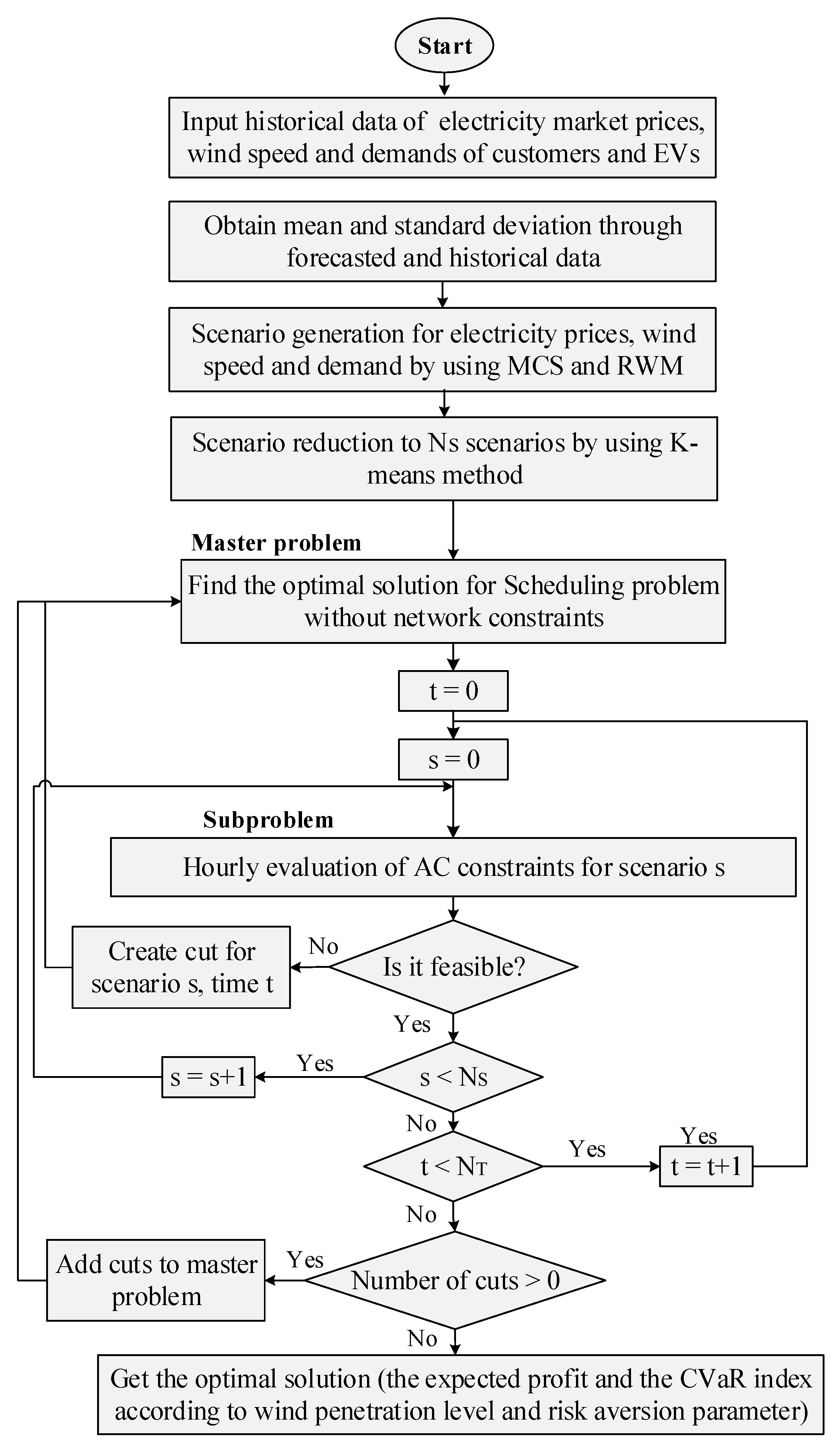
2.6. Solution Methodology

Figure 1 depicts the flowchart of the proposed algorithm for solving the optimal scheduling model considering wind power generation and DR programs. At first, forecasted value of the uncertain parameters including electricity prices and wind power, as well as EVs’ and customers’ demand is obtained by using traditional forecasting techniques. The forecast errors are modeled through appropriate probability density functions (PDFs) and a set of scenarios are then generated based on PDFs using Monte-Carlo simulation (MCS) and roulette wheel mechanism (RWM) [22]. Since the generated scenarios directly influence the computational complexity and due to the computational limitations in the scheduling problem, in this work, the K-means classification method [23] is used to decrease the number of scenarios to a limited set which adequately represents the uncertainties. In the next stage, the reduced scenario set is used in the scheduling problem that is decomposed into a master problem and a sub-problem.

The master problem determines the optimal schedule of dispatchable units, interactions with the main grid as well as adjustable loads and EVs demand in a mixed-integer programming (MIP)-based problem. The obtained binary solution will be used in the sub-problem to evaluate AC constraints in scenarios. If the solution does not satisfy a predefined optimality criterion, for example, power mismatches are not zero, the optimality cut is generated and added to the master problem for revising the current schedule. The optimality cut is denoted in the form of an inequality constraint, which provides a higher estimation of the expected profit as a function of scheduling variables in the master problem.

3. Simulation and Numerical Results

3.1. Case Study

To test the feasibility of the proposed method, the simulations are performed for a typical microgrid in grid-connected mode which is shown in Figure 2. The microgrid consists of six similar wind turbines, five dispatchable generation units (including two micro-turbines (MT₁ and MT₂), two fuel cells (FC₁ and FC₂) and one diesel engine (DE)), eight groups of responsive loads and two EVs parking lots (PLs). The characteristic of dispatchable units are extracted from reference [24]. Six wind turbines that the capacity of each one is 80 kW, are installed at buses 5, 9 and 15. Here, the proposed problem is solved for one day, which is divided into 24 time periods. The hourly forecasted power of wind generation, demand of customers and EVs as well as DA electricity prices (extracted from Nordpool market) are shown in Figure 3 [25].

The initial SOC of EVs at each scenario is randomly generated. The forecast errors of stochastic parameters are modeled using their associated PDFs in which the mean values are equivalent to the forecasted values of related variables. Standard deviation of the forecast errors associated with industrial loads, EVs demand, DA market prices are considered ±10% [24,26]. Also, the price elasticity of the loads can be found in reference [15]. Subsequently, a number of 1000 initial scenarios representing plausible realization of stochastic processes on the scheduling horizon are generated using MCS and RWM mechanisms. In order to render the proposed scheduling problem tractable, the number of scenarios is trimmed down using K-means algorithm as an appropriate scenario-reduction algorithm. In the next step, the scheduling problem is solved for the selected scenarios to maximize the expected profit of the microgrid operator. The problem is implemented with a personal computer with 4 GB RAM and Intel Core i7 @ 2.60 GHz processor using CPLEX 11.0 [27].

3.2. Numerical Results

The scheduling problem is solved while considering different levels of wind power penetration and different values of the weighting parameter β. Figure 4a–c shows the efficient frontiers for three levels of wind capacity i.e., 0, 50% and 100%, respectively. In this study, the confidence level to compute CVaR is considered 95% in all instances. Also, the optimal solution of the problem is shown only for nine values of risk aversion β by modifying this parameter from 0 (risk-natural case) to 25 (risk-averse case) as observed in this Figure. As observed, by growing β, the total expected profit of the operator decreases and CVaR, which shows the average of expected profit over the worst-case scenarios increases in different wind penetration levels. At the risk-natural case (e.g., β = 0), the maximum profit at minimum CVaR is attained.

If parameter β increases from 0 to 25, the expected profit decreases 85% and 7.5% for wind penetration level of 0 and 100%, respectively. However, when β increases from 0 to 25, CVaR increases 39.8% and 19% for the mentioned wind penetration levels, respectively. The results indicate that by increasing the level of wind power in the microgrid, the dependency between expected profit and the risk-averse behavior of the operator reduces. In other words, with a lower level of wind power, the expected profit is highly dependent on the risk-aversion of the microgrid operator. This is a consequence of the fact that in the case of a low level of wind power penetration, the operator supplies more power from upstream. Trading energy with the upstream causes the occurrence of more undesirable scenarios. Since, the standard deviations of electricity price forecasts are considered higher than that of the wind power [16], trading energy with the upstream might cause the occurrence of more undesirable scenarios. Therefore, in low level of wind power, the effect of risk aversion factor on the expected profit is significantly high.

Figure 5 depicts the impact of penetration level of wind power in different values of β on the expected profit, cost of generation and CVaR. It is observed that the expected profit is monotonically increased as the wind power penetration in the system is increased due to the negligible cost of wind generation. Even if the cost of wind power is non-zero, the same argument can be made as such a cost is much less than the cost of conventional power generation. Therefore, with increasing wind power penetration, a few units are dispatched and thus the operating cost decreases (see Figure 5b), and the expected profit of the operator increases significantly. On the other hand, the system cost is not only affected by wind power penetration levels but also by risk aversion behavior of the operator. The operational cost of dispatchable units under different risk and wind penetration levels are shown in Figure 5b. Since in higher risk aversion, the operator tries to purchase high amount of the required energy from more reliable dispatchable units, supplying power from them increases. In fact, providing energy from dispatchable units has less volatility rather than providing it from electricity market. Therefore, as it was shown before, by increasing β, trading energy between the microgrid and main grid decreases and the operator tries to supply high amounts of energy from dispatchable units. Also, it can be observed from Figure 5c that when the wind power penetration level is augmented, the CVaR term reduces.

In higher penetration level of wind power, uncertainties of energy resources increase which in turn necessitate actions for risk reduction. This implies a profit loss to the system operator. In fact, by increasing the risk aversion parameter, the profit in the best scenario decreases while the opposite happens in the worst scenario. Therefore, a risk-averse operator is willing to sacrifice high profits in the best scenarios in the hope of avoiding profit loss or low profit in worst scenarios. Figure 6 shows the cost of trading energy between the microgrid and the main grid in different wind power penetration levels and in three levels of risk. As shown, when wind power penetration increases, the amount of energy imported from the main grid decreases. At the same time, with higher wind power penetrations, cheaper energy blocks are available which help the operator to sell extra energy to the main grid and making more profit. Also, in a risk-neutral case, the operator tends to buy more energy blocks from the main grid and therefore it has the highest payment and the lowest achievement for energy trading with the main grid. In contrast, in a risk-averse case, the operator supplies microgrid loads from more reliable dispatchable units rather than the main grid, and as a result, it buys few energy blocks from the main grid while exporting energy to it most of the time to make more profit. In a risk-averse case, the operator tends to buy few energy blocks from the main grid while it often sells energy to it.

Figure 7 illustrates the cost of trading energy between the microgrid and main grid versus risk-aversion parameter β. As shown, in lower risk levels, cost of purchasing energy from the main grid is the highest and most of loads are supplied by the main grid. However, when β shifts, the operator provides more energy from the local dispatchable units to hedge against the volatility of the electricity market. To get better insight into the trading mechanism, the hourly energy exchange between the microgrid and the main grid is depicted in Figure 8, for different levels of wind penetration. As shown, by increasing the wind penetration level, the trading pattern changes most of the time and in most cases. Specially, higher penetration rates result in more energy being exported to the main grid regardless of the risk-aversion level. As an example, with a wind penetration level at around 50% or above, the energy is exported to the main grid, especially during 10:00 to 16:00 when the DA market prices are relatively high and there is enough wind power production. However, during the off-peak periods when DA market prices are low, the microgrid operator prefers to supply part of the load through the main grid at lower costs, even with 100% wind penetration (see Figure 8c).

4. Conclusions

This paper presented a risk-constrained stochastic model for the scheduling of a hybrid grid-connected microgrid with flexible demand-side resources and wind power generation in both an energy and reserve market. The proposed model also captured uncertainties associated with DA market prices, demand loads, power of EVs as well as the wind power generation in energy and reserve scheduling process. Also, to hedge against profit volatilities, a CVaR metric was incorporated into the objective function. The validity of the proposed model was investigated and supported by mathematical analysis and simulation. The effects of wind power penetration level and risk-aversion of the operator on the optimal solution of the scheduling problem was also assessed. The results showed that by increasing the wind power penetration level in the microgrid, the profit and CVaR dependency on the risk-aversion of the operator reduces. Moreover, the results demonstrated that in a certain risk level with a high penetration of wind energy, a lower operation cost could be obtained by balancing the economics and the operational risks when accommodating wind power variations.

References

1. Rashidizadeh-Kermani, H.; Vahedipour-Dahraie, M.; Shafie-khah, M.; Catalão, J.P.S. A Bi-level risk-constrained offering strategy of a wind power producer considering demand side resources. Int. J. Electr. Power Energy Syst. 2019, 104, 562–574. [Google Scholar] [CrossRef]
2. Sáiz-Marín, E.; Lobato, E.; Egido, I. New challenges to wind energy voltage control. Survey of recent practice and literature review. IET Renew. Power Gener. 2018, 12, 267–278. [Google Scholar] [CrossRef]
3. Vahedipour-Dahraie, M.; Najafi, H.R.; Anvari-Moghaddam, A.; Guerrero, J.M. Security-constrained unit commitment in AC microgrids considering stochastic price-based demand response and renewable generation. Int. Trans. Electr. Energy Syst. 2018, 28, e2596. [Google Scholar] [CrossRef]
4. Vahedipour-Dahraie, M.; Najafi, H.R.; Anvari-Moghaddam, A.; Guerrero, J.M. Study of the effect of time-based rate demand response programs on stochastic DA energy and reserve scheduling in islanded residential microgrids. Appl. Sci. 2017, 7, 378. [Google Scholar] [CrossRef]
5. Anvari-Moghaddam, A.; Guerrero, J.M.; Vasquez, J.C.; Monsef, H. Efficient energy management for a grid-tied residential microgrid. IET Gener. Trans. Distrib. 2017, 11, 2752–2761. [Google Scholar] [CrossRef]
6. Rashidizadeh-Kermani, H.; Vahedipour-Dahraie, M.; Najafi, H.R.; Anvari-Moghaddam, A.; Guerrero, J.M. A stochastic Bi-level scheduling approach for participation of EV aggregators in competitive electricity markets. Appl. Sci. 2017, 7, 1100. [Google Scholar] [CrossRef]
7. Rashidizadeh-Kermani, H.; Najafi, H.R.; Anvari-Moghaddam, A.; Guerrero, J.M. Optimal decision-making strategy of an electric vehicle aggregator in short-term electricity markets. Energies 2018, 11, 2413. [Google Scholar] [CrossRef]
8. Waqquas, A.; Zhang, C.; Pinson, P. An integrated multiperiod OPF model with demand response and renewable generation uncertainty. IEEE Trans. Smart Grid 2016, 7, 1495–1503. [Google Scholar]
9. Yang, S.; Zeng, D.; Ding, H.; Yao, J.; Wang, K.; Li, Y. Stochastic security-constrained economic dispatch for random responsive price-elastic load and wind power. IET Renew. Power Gener. 2016, 10, 936–943. [Google Scholar] [CrossRef]
10. Wanga, D.; Qiub, J.; Reedman, L.; Meng, K.; Lai, L.L. Two-stage energy management for networked microgrids with high renewable penetration. Appl. Energy 2018, 226, 39–48. [Google Scholar] [CrossRef]
11. Lahon, R.; Gupta, G.C. Risk-based coalition of cooperative microgrids in electricity market environment. IET Gener. Transm. Distrib. 2018, 12, 3230–3241. [Google Scholar] [CrossRef]
12. Rodrigues, T.; Ramírez, P.J.; Strbac, G. Risk-averse bidding of energy and spinning reserve by wind farms with on-site energy storage. IET Renew. Power Gener. 2018, 12, 165–173. [Google Scholar] [CrossRef]
13. Mohammad, N.; Mishra, Y. Coordination of wind generation and demand response to minimise operation cost in day-ahead electricity markets using bi-level optimization framework. IET Gener. Transm. Distrib. 2018, 12, 3793–3802. [Google Scholar] [CrossRef]
14. Paterakis, N.G.; de la Nieta, A.A.S.; Bakirtzis, A.G. Effect of risk aversion on reserve procurement with flexible demand side resources from the ISO point of view. IEEE Trans. Sustain. Energy 2017, 8, 1040–1050. [Google Scholar] [CrossRef]
15. Vahedipour-Dahraie, M.; Najafi, H.R.; Anvari-Moghaddam, A.; Guerrero, J.M. Stochastic security and risk-constrained scheduling for an autonomous microgrid with demand response and renewable energy resources. IET Renew. Power Gener. 2017, 11, 1812–1821. [Google Scholar] [CrossRef]
16. Vahedipour-Dahraie, M.; Anvari-Moghaddam, A.; Guerrero, J.M. Evaluation of reliability in risk-constrained scheduling of autonomous microgrids with demand response and renewable resources. IET Renew. Power Gener. 2018, 12, 657–667. [Google Scholar] [CrossRef]
17. Sharifi, R.; Anvari-Moghaddam, A.; Fathi, S.H. Economic demand response model in liberalized electricity markets with respect to flexibility of consumers. IET Gener. Trans. Distrib. 2017, 11, 4291–4298. [Google Scholar] [CrossRef]
18. Sharifi, R.; Anvari-Moghaddam, A.; Fathi, S.H. Dynamic pricing: An efficient solution for true demand response enabling. J. Renew. Sustain. Energy 2017, 9, 065502. [Google Scholar] [CrossRef] [Green Version]
19. Carrión, M.; Arroyo, J.M.; Conejo, A.J. A bilevel stochastic programming approach for retailer futures market trading. IEEE Trans. Power Syst. 2009, 24, 1446–1456. [Google Scholar] [CrossRef]
20. Heydarian-Forushani, E.; Moghaddam, M.P.; Sheikh-El-Eslami, M.K.; Shafie-Khah, M. Risk-constrained offering strategy of wind power producers considering intraday demand response exchange. IEEE Trans. Sustain. Energy 2014, 5, 1036–1047. [Google Scholar] [CrossRef]
21. Geramifar, H.; Shahabi, M.; Barforoshi, T. Coordination of energy storage systems and demand resources for optimal scheduling of microgrids under uncertainties. IET Renew. Power Gener. 2017, 11, 378–388. [Google Scholar] [CrossRef]
22. Rashidizadeh-Kermani, H.; Vahedipour-Dahraie, M.; Anvari-Moghaddam, A.; Guerrero, J.M. Stochastic risk-constrained decision-making approach for a retailer in a competitive environment with flexible demand side resources. Int. Trans. Electr. Energy Syst. 2019, 29, e2719. [Google Scholar] [CrossRef]
23. Arthur, D.; Vassilvitskii, S. K-means++: The advantages of careful seeding. In Proceedings of the 18th Annual ACM-SIAM Symposium Discrete Algorithms (SODA’07), New Orleans, LA, USA, 7–9 January 2007; pp. 1027–1035. [Google Scholar]
24. Rezaei, N.; Kalantar, M. Economic–environmental hierarchical frequency management of a droop-controlled islanded microgrid. Energy Convers. Manag. 2014, 88, 498–515. [Google Scholar] [CrossRef]
25. Relevant Information on the Market Pertaining to Nordpool. Available online: http://www.Nordpool.com (accessed on 5 September 2016).
26. Rezaei, N.; Kalantar, M. Smart microgrid hierarchical frequency control ancillary service provision based on virtual inertia concept: An integrated demand response and droop controlled distributed generation framework. Energy Convers. Manag. 2015, 92, 287–301. [Google Scholar] [CrossRef]
27. The General Algebraic Modeling System (GAMS) Software. Available online: http://www.gams.com (accessed on 15 September 2016).
Figure 1. Flowchart of the proposed algorithm for solving the optimal scheduling model.
Electronics 08 00577 g001
Figure 2. Schematic diagram of the microgrid being studied.
Electronics 08 00577 g002
Figure 3. The hourly forecasted values of (a) customers’ loads, charging demand of electric vehicles (EVs) and wind power and (b) day-ahead (DA) electricity price.
Electronics 08 00577 g003
Figure 4. Operator’s expected profit versus conditional value-at-risk (CVaR) in different wind penetration levels: (a) Wind penetration level = 0%; (b) Wind penetration level = 50%, and (c) Wind penetration level = 100%.
Electronics 08 00577 g004aElectronics 08 00577 g004b
Figure 5. Impact of wind power penetration level at different values of β on (a) expected profit, (b) cost of generation, and (c) CVaR.
Electronics 08 00577 g005aElectronics 08 00577 g005b
Figure 6. Cost of trading energy versus wind penetration level (a) buying from main grid; (b) selling to the main grid.
Electronics 08 00577 g006
Figure 7. Cost of trading energy versus risk aversion parameter (a) buying from the main grid, (b) selling to the main grid.
Electronics 08 00577 g007
Figure 8. Hourly energy trading between the microgrid and the main grid in different penetration levels of wind power, (a) penetration level = 0%, (b) penetration level = 50%, and (c) penetration level = 100%.
Electronics 08 00577 g008aElectronics 08 00577 g008b