Optimal Scheduling Strategy of Distribution Network Based on Electric Vehicle Forecasting


1
Institute of Electrical Engineering, Yanshan University, Qinhuangdao 066004, China
2
Institute of Advanced Technology, Nanjing University of Posts and Telecommunications, Nanjing 210023, China
3
State Key Laboratory of Power Grid Safety and Energy Conservation, China Electric Power Research Institute, Haidian District, Beijing 100192, China
*
Author to whom correspondence should be addressed.
Electronics 2019, 8(7), 816; https://doi.org/10.3390/electronics8070816
Submission received: 18 June 2019
/
Revised: 18 July 2019
/
Accepted: 19 July 2019
/
Published: 22 July 2019
(This article belongs to the Special Issue Advances in Power Electronics Technologies for Renewable Energy Systems)
Abstract
:Based on the Monte Carlo method, this paper simulates, predicts the load, and considers the travel chain of electric vehicles and different charging methods to establish a predictive model. Based on the results of electric vehicle simulation prediction, an optimal scheduling model of the distribution network considering the demand response side load is established. The firefly optimization algorithm is used to solve the optimal scheduling problem. The results show that the prediction model proposed in this paper has a certain reference value for the prediction of an electric vehicle load. The electric vehicle is placed in the optimal scheduling resource of the distribution network, which increases the dimension of the scheduling resources of the network and improves the economics of the distribution network operation.
1. Introduction
In the context of energy shortages, severe environmental pollution, and global climate change [1,2], electric vehicles (EVs) are alleviating the energy crisis and promoting human and natural sustainability as a representative of a new type of green transportation vehicle. Development and other aspects have the incomparable advantages of traditional fuel vehicles, and have been highly upheld by governments, auto manufacturers, and energy companies [3]. However, due to the uncertainty and mutual differences between the demand and behavior of EV users, the large-scale EV charging load in the future has uncertain characteristics, such as randomness, intermittency, and volatility in time and space [4,5], and it will affect the grid. The safe operation and optimization of scheduling bring difficulties [6], and it is required to establish an effective EV charging load forecasting model to provide theoretical support for analysis of the impact of EV charging loads and laying the foundation for power grid and operational planning.
The uncertainty of EVs puts new demands on the optimal scheduling of distribution networks. On the one hand, because the accuracy of the prediction error of the load is related to the time scale, it is difficult to meet the scheduling requirements of the system [7]. On the other hand, various types of EV load-preferred demand side resources [8] participating in the scheduling have multi-time-scale characteristics, and the prediction accuracy is also low, making it difficult to make full use of each demand side resource. Therefore, these make it difficult to optimize the scheduling of the distribution network.
At present, many scholars have studied the prediction of EVs, and on this basis, optimized the resources in the distribution network. Reference [9] only simulated the charging load of a single EV, and was able to obtain the daily load curve. It only considered the same type of private car, and assumed that each charge was full, so there was a certain error between the simulation results and the actual situation. Reference [10] discussed the types of EV and the corresponding charging methods and times, but it did not consider the spatial distribution prediction problem of the load, and the prediction result was lacking in accuracy. Reference [11] proposed an optimization strategy to consider the decentralized charging of EVs. In the case of user competition, it will play a certain role in suppressing peak-to-valley differences. Reference [12] fully considered the process of charging and discharging EVs, and proposed a global and local optimal charging optimization strategy. Reference [13] studied the centralized charging strategy under the influence of time-sharing electricity prices. However, they did not consider the space–time distribution characteristics of the user’s electricity consumption, and did not give prediction information for the EV’s starting charging time and initial power. Reference [14] constructed a spatiotemporal distribution model of the EV charging load by using a model simulation method. Reference [15] proposed a space–time prediction method for charging loads based on the driving and parking characteristics of EVs. Reference [16] proposed a space–time distribution model of charging loads based on residents’ travel chains. In Reference [17], in order to cope with the randomness of the demand side output, a pre-optimization scheduling model of the distribution network was established to effectively ensure the safe and stable operation of the distribution network. In Reference [18], a scheduling model combining day-to-day scheduling, intra-day rolling scheduling, and real-time scheduling was proposed. The time-scale was refined step by step to eliminate the influence of wind power prediction error on distribution network optimization. In Reference [19], a robust optimization model was established to coordinate the output of energy storage and other reactive devices, as well as to achieve active/reactive joint optimization scheduling of the distribution network. Reference [20] considered the basic constraints of the distribution network, and studied the impact of demand response (DR) resources on the reliability of the distribution network power supply. Reference [21] modeled the demand response and integrated load, and studied the application examples of an active distribution network. The above literature considered the prediction of electric vehicles and the optimal scheduling of distribution networks, but they were all separate, and the combination of the two was rare. References [22,23] both considered energy scheduling based on model predictive control, in which the receding horizon principle could be used to deal with the uncertainty of scheduling parameters. Reference [24] presented a distributed waterfilling algorithm for networked control systems, and applied it to a case study on the charging of a fleet of electric vehicles. The algorithm are fully distributed and scaled to large-scale situations. Reference [25] addressed the problem to control a population of noncooperative heterogeneous agents, and studied charging coordination for Plus-in Electric Vehicles with transmission line constraints. The proposed method is innovative.
This paper presents EV load forecasting modeling based on the Monte Carlo simulation, starting with the travel chain of EVs and different charging methods. The Monte Carlo method is used to deal with randomness and uncertainty in the operation of electric vehicles. The proposed travel chain includes a large amount of related features in time and space; thus, it is helpful to the accuracy of forecasting results. Secondly, on this basis, the EV is connected to the distribution network as a demand consideration, and an optimal scheduling model of the distribution network is established to analyze the optimization results of the distribution network with or without EV access. The firefly algorithm is considered a population-based algorithm, because the search process is simple and easy to implement; thus, it is used to solve the optimization problems above. The firefly algorithm takes a very short time, which is much less than the planning step, i.e., 1 h, so it can be regarded as on-line optimization in the paper.
2. EV Load Forecasting Modeling Based on Monte Carlo Method
EVs mainly include private cars, buses, taxis, and so forth. Charging methods can be divided into the following groups—slow charging, fast charging, and vehicle battery replacement—and charging locations are generally at charging stations and parking lots. This paper focuses on modeling the charging load of private car analysis. Due to the lack of reliable historical data related to the current travel characteristics of electric vehicle users, it is assumed that electric vehicles have similar travel characteristics as conventional fuel vehicles.
This paper predicts the overall modeling of electric vehicle charging loads, as shown in Figure 1.
3. EV Load Forecasting Model
3.1. EV Travel Chain
The travel chain includes the starting point, ending point, parking location, driving route, start time, end time, and parking time of each travel activity. The process of the user starting from home, going everywhere he likes, and finally returning home is described in a general sense, including a large amount of related features in time and space.
Figure 2 depicts a random travel route. If each travel destination is treated as a state, the next state (destination) of the vehicle is determined by the current state. Assuming that the vehicle is currently in state , then at the next moment, it may be from state to any of the states of . Note that is the state transition probability from state to state , then, satisfies the condition:
Figure 3 is a corresponding schematic diagram of a travel chain, where the broken line indicates the running process, the solid line indicates the parking process, the solid point indicates the start and end time of the day’s travel, and the hollow point indicates the arrival and departure time of each place. , are the moments of arrival at the destinations and , respectively; , are the moments of leaving the destinations and , respectively; , are the parking times for the destinations and , respectively; , are the first and last travel times of the day, respectively; and is the travel time from destination to destination .
It can be seen from the diagram of the travel chain, that each travel process is only related to the previous travel destination, which can be regarded as there being no after-effectiveness.
3.2. EV Charging Load Distribution Forecast
3.2.1. Determination of the Charging Method of EVs
The charging method was divided into DC fast charging and AC slow charging, and battery charging replacement was not considered in this paper. For different functional areas and vehicles, the initial charging time differed when different charging methods were used. Assume that the private car is charged regularly after returning home for the last time, and that fast charging is used as an emergency backup mode.
(1) The user arrives at the parking place, and will charge if the remaining battery power is insufficient to support the next destination. At this time, you can choose fast charging or slow charging; during the parking time, if slow charging is not enough to drive to the next destination, then use fast charging—otherwise, use slow charging. That is, when the user arrives at the first parking place, fast charging is only used when the following formula is satisfied:
where is the slow charging power, kW; is the remaining power when reaching the first destination, kW·h; is the electric power consumption per kilometer of the EV, kW·h/km; is the battery capacity, kW·h, considering factors such as battery safety and user psychology, where the state of charge (SOC) of the EV is not less than 20%. is the distance from destination to the next destination, .
When the vehicle reaches a certain destination, the state of charge of the battery is as follows:
where is the state of charge of the battery of the EV at time ; is the initial state of charge; is the starting time of the EV; is the daily driving range; is the daily average driving time; and is the EV’s maximum cruising range.
(2) If the remaining battery capacity can support driving to the next destination, the user can choose to charge slowly or not. Let the initial state of charge, obey the normal distribution, . After each stop, extract a random number from to represent the starting of the user’s habit (denoted as ), compared with the current remaining of the electric car (denoted as ). If , it means that the current remaining power of the user is greater than expected, and the user does not choose to charge; otherwise, the remaining power is less than what the user is accustomed to in regard to the charging starting power, and the user selects slow charging.
3.2.2. Calculation of EV Charging Load
Firstly, the forecast area is divided into blocks and functional lands, such as residential, office, and entertainment areas. When the vehicle reaches a certain function land, I, it is judged whether it is charged according to the state of charge of the battery. When determining to charge, firstly, the charging mode to be used is determined, and then, according to different charging methods, the initial charging time of the vehicle is extracted. After this, the number of EVs charged by different charging methods is accumulated, and the proportion of different charging methods is determined by numerical calculation. Finally, the Monte Carlo simulation is used to calculate the overall charging load of different functional areas in the predicted area for one day. The simulation flow is shown in Figure 4.
For private cars, slow charging mostly occurs when the user returns home at the end of the day’s trip. The initial charging time of the vehicle is related to the electricity price policy, the user’s charging habits, and driving demand. represents the probability density of the initial charging time in slow mode, where it obeys the piecewise normal distribution:
where , are the expectation and variance of the charging start time, respectively.
For private cars, the slow charging mode is the preferred method, while the fast charging mode is only used to meet the emergency backup charging. Compared with slow charging, the fast charging time has obvious randomness. If an EV arrives at destination at time and leaves at time , then the probability density of the initial charging time in fast mode is expressed by ; then approximately satisfies the uniform distribution, which can be expressed as:
where is the ratio of different charging intervals.
In practical applications, the battery pack residual power of the electric vehicle in the station varies, which makes the charging time long or short. The charging time length approximately obeys a normal distribution, described as follows:
where , are the expectation and variance of the charging time length, respectively.
When the EV arrives at the destination , the probability of charging at time is:
where is the charging probability of the car arriving at the destination for the hour; is the joint probability distribution function of the charging start time and the charging time length, and they are independent of each other, so , is the probability distribution function of the charging start time, and is the probability distribution function of the charging time length. is the charging start time when the EV arrives at destination , and is the charging time length.
Therefore, at the period, the charging load of the I-zone EV using the slow charging mode is:
The charging load of electrical vehicles using the fast charging mode in function area I at time is:
where and are the slow and fast charging loads at the hour at destination , respectively; and represent the numbers of slow charging and fast charging of the EVs at the hour, respectively; and are slow and fast charging powers, respectively. The load of the M functional lands was accumulated to obtain the total charging load of the I functional areas at the hour:
3.3. EVs Send Power to the Electric Grid
Vehicle-to-grid (V2G) describes a system where battery, hybrid, and fuel cell vehicles can all send power to the electric grid. Electric vehicles charge from the grid at night when the electricity demand is small and the electricity price is low.
When the daytime demand for electricity is large and the price is high, the electric vehicle will feed back the electricity to the power grid, which can provide peak-shaving and valley-filling services to balance daily electric load and mitigate the duck curve. It can buffer the intermittent renewable energy access to the power grid. In case of strong wind, excessive wind power is stored in the batteries of electric vehicles and fed back to the power grid at peak load, thus playing a stable role in intermittent wind energy.
4. Distribution Network Optimization Scheduling
The energy grid optimization of the distribution network determines the price of the day based on the previous output of the new energy and forecast data of the EV load. Based on this, the power consumption and quotation of the demand side resources that can respond to the scheduling are used to meet the safety constraints. Under the condition, with the minimum operating cost of the distribution network as the goal, the output of each micro-source and the demand-side resources will be scheduled. The real-time scheduling is still based on the safe and stable operation of the distribution network. The demand side resources and the rotating reserve are directly controlled as the adjustment amount, and the operation cost of the distribution network is the minimum. The optimization of each part is the constraint construction optimization model.
4.1. Distribution Network Optimization Scheduling Model
Reference [21] presented a decentralized control strategy for the scheduling of electrical energy activities of a microgrid. Optimally planning users’ controllable loads is useful in reducing the costs. Reference [26] presented a method for tracking a secondary frequency control signal by groups of plug-in hybrid electric vehicles (PHEVs), as well as controllable thermal household appliances. It was illustrated that load frequency control, used as an equivalent to secondary control, can be effectively provided by loads, such as PHEVs and household appliances. In our paper, the electric vehicles can be regarded as shiftable loads, and the interruptible load as a controllable load. Controllable loads can be given a different priority according to the actual situation for scheduling.
Assuming that the new energy output value is known and the energy storage of electric vehicles has been predicted by the Monte Carlo method, which can be dominantly used in optimization problems, the other demand side resources are adjusted to target the total operating cost of the distribution network. The objective function and constraints are as follows:
(1) Objective function:
(2) Constraints:
Power balance constraint:
The wind power output is known, and its constraint is:
The photoelectric output is also known, and its constraint is:
Interactive power constraint:
Electrical vehicle total load constraint:
Interruptible loads constraint:
Energy storage constraint [27,28]:
where and are the wind and photovoltaic power at time , respectively; and are the power consumption of wind and photovoltaic power per kW·h at time , respectively; and are the serial number and total of wind turbines, respectively; and are the serial number and total number of PV modules, respectively; and are the interaction power and purchase price of the distribution network and the large grid, respectively; is the comprehensive cost of the energy storage equipment; is time-of-use price; and are the serial number and the total number of interruptible loads in response to the schedule, respectively; is the call price of the interruptible load actually participating in the schedule per kW·h at time ; and are the minimum and maximum powers of wind power generation, respectively; and are the minimum and maximum powers of photovoltaic power generation, respectively; and are the lower and upper limits of the exchange power between the distribution network and large power grid, respectively; is the amount electricity of EVs to be called; is the amount of load called; and are charging and discharging powers of the battery, respectively; and are the minimum charging and the maximum discharging powers of the battery, respectively; is the charging or discharging time length; and , are the minimum and maximum values of adjustable EVs’ energy storage, respectively.
The problem we need to solve is the optimization problem with constraints. The decision variables are real-type ones, and include , , , , and . Equation (13) is a constraint of equality, and the other Equations (14)–(19), are the bounding constraints.
4.2. Firefly Optimization Algorithm
Here, the firefly algorithm is proposed to simulate the natural phenomenon where fireflies in nature gather at night. This is a heuristic group intelligent optimization algorithm [17]. The algorithm regards the points in the search space as firefly individuals, and uses the strong fireflies to attract the characteristics of the weakly fired fireflies. In the process of moving the weak individuals to the strong individuals, the iteration of the position is completed. The iterations find the optimal position and complete the optimization. This algorithm is used to solve the optimal scheduling model of the distribution network.
Luminous brightness of firefly :
where is the position of the firefly individual in the d-dimensional space, here being the solution of each scheduling model of the distribution network; is the calculation function of the brightness of the firefly. Here, the objective function of each scheduling model of the distribution network is used as the fitness function, and is used to indicate the brightness of the firefly.
Attraction between firefly individuals and :
where is the maximum attractiveness of the light source, 1; is the light absorption coefficient; and is the Cartesian distance between fireflies and , expressed as follows:
When firefly is attracted to firefly , its position update formula is expressed as:
where and are the positions of firefly individuals and at iterations; is the step factor; and is the random number vector obeying the Gaussian distribution at the iteration.
In this paper, the fitness value is used to indicate the brightness of the firefly. The firefly constantly update the position and be attracted to find the best one until the stop condition is met, then the firefly with the brightest light is obtained, that is, the firefly with the largest value of the fitness function is located. So the best scheduling solution is obtained.
5. Case Study
In order to verify the validity of the model established in this paper, simulation analysis was performed by MATLAB. Firstly, the EV load was predicted, and on this basis, the optimal scheduling analysis of the distribution network connected to the EV was carried out.
This paper mainly forecasts the charging load of EVs in the Zhengzhou Economic Development Zone, China, in the summer. According to the city’s EV development plan, it is predicted that the number of electric private cars will be 52,000 in 2030. According to the survey, the average daily mileage of private cars in the area is 33.85 km. The vehicle uses lithium batteries, where it is assumed that each charge is full; the charging efficiency is 90%, and the minimum threshold value of the battery charging state is 20%. The charging interface power is regulated according to the “Connecting device for conductive charging of EVs” and Table 1.
The Monte Carlo simulation method was used to calculate the charging load curve of the private car. The prediction results are shown in Figure 5 and Figure 6.
(1) Comparison of charging load in different functional areas. Due to the different nature of land used in different functional areas, the spatial distribution and charging time of EVs are different. It can be seen from the analysis of Figure 5, Figure 6 and Figure 7 that the charging loads of different functional sites differ greatly, and the peak load and peak time are also different. The residential area mainly satisfies the nighttime charging behavior of private car owners. Therefore, the peak load occurs from 19:00 to 24:00. The charging load in the work area is mainly concentrated in the working hours of 10:00–16:00, while the charging load in the commercial area is mainly concentrated in the working hours of 8:00–20:00. It can be concluded that the charging load is closely related to the spatial position.
(2) Comparison of charging load under different charging modes. According to the parameters of the two main models given in this chapter, the quick charge ratio is 0.239 when the model with a smaller battery capacity is selected. As the battery capacity increases, the fast charge ratio decreases to 0.097, which results in different fast charge ratios. The load curve is shown in Figure 5. It can be seen from Figure 6 that when the fast charge ratio is 23.9%, the peak value of the load curve increases, which has a greater impact on the power grid, increasing the pressure on the distribution network in the area. It can be seen that with the increase of the cruising range of the EV, the vehicle owner adopts the fast charge. The proportion is reduced, so that the impact of the charging load on the grid is also reduced.
On the basis of the EV load forecast, the EV was connected to the distribution network as the load on the demand side. The parameter algorithm was set by adding the constraints of each scheduling resource in the distribution network optimization model. The optimal scheduling model based on EV load forecasting and considering the demand side response was solved, and the optimal scheduling scheme of the distribution network was obtained.
According to the survey, in the distribution network with new energy generation, the cost of wind power generation is 0.55 ¥/kW·h, and the combined cost of photovoltaic power generation is 0.45 ¥/kW·h. The estimated total discharge cost is 1.2 ¥/kW·h by estimating the service life of the battery. The distributed energy network parameters are shown in the Table 2.
The SOC value of the battery energy storage in this paper ranges from 0.2 to 0.9, and its charge and discharge efficiency is approximately 0.9. The electricity purchase price of the distribution network to the large power grid is changed according to the time-sharing electricity price of the large power grid. The time-of-use electricity price is shown in Table 3. The peak electricity price is the highest, and the night load is the lowest, so the electricity price is the lowest.
The compensation prices of various types of interruptible load resources and EVs that can participate in the demand side response in the system are shown in Table 4, and include the upper and lower limits of their response capacity. Since the impact of the interruptible load is relatively large, the maximum interruption time is generally 4 h. In Table 4, the EV is owned by the owner. In addition to meeting the call of the distribution network, the owner should ensure the normal use of the EV. It is assumed here that after all the EVs arrive at the destination, 73% of the energy is left in the car battery; when the car leaves the location, the remaining energy in the battery should have 33% of the capacity. The compensation price for all response schedule EVs is 0.1¥/kW·h. Table 4 shows the compensation price when the EV responds to the schedule discharge.
The optimal scheduling scheme of the distribution network when the EV is connected to the distribution network and participates in optimal scheduling is shown in Figure 7.
The optimal scheduling scheme of the distribution network for when the EV does not participate in the optimal scheduling of the distribution network is shown in Figure 8.
It can be seen from the above two scheduling schemes that it is difficult for the distribution network to meet the requirements including economy, when the load is at a peak period, if EVs do not participate in the scheduling. The participation of EVs reduces the operating costs of the distribution network. Two different scheduling schemes and power generation costs are shown in Table 5.
6. Conclusions
In this work, the EV load forecasting was put forward, and the optimal scheduling strategy of distribution network was also proposed. The effectiveness of the proposed strategy was verified by simulation. The main conclusions are as follows:
(1) By analyzing the travel chain and charging mode of EVs, a load forecasting model for EVs was established. Then, forecasting of the EV load was accomplished based on the Monte Carlo method.
(2) The EV was placed in the scheduling resources of the distribution network with new energy power generation. The addition of the EV saves the operating cost of the distribution network and increases the dimension of the scheduling resources of the distribution network.
Research on the optimal scheduling of the distribution network for accessing EVs in the future mainly focuses on solving the bidding mechanism of load agents and the compensation mechanism of EV calls. Through reasonable compensation of the price, to ensure that the EV is connected to the distribution network, the demand side resources can actively respond to the scheduling of the distribution network to maximize the total social welfare.
Author Contributions
Investigation, F.L.; supervision, C.D. and S.X.
Funding
This work is supported by the Key projects of the National Natural Science Foundation of China under Grant 61833008, National Natural Science Foundation of China under Grants 61573300 and 61533010, Jiangsu Provincial Natural Science Foundation of China under Grant BK20171445, Key research and development plan of Jiangsu Province-Industrial foresight and common key technical projects under Grant BE2016184, Hebei Provincial Natural Science Foundation of China under Grant E2016203374.
Acknowledgments
The authors gratefully acknowledge the helpful comments and suggestions of editors and anonymous reviewers.
Conflicts of Interest
The authors declare no conflict of interest.
References
- Song, Y.H.; Yang, X.; Lu, Z.X. Integration of plug-in hybrid and electric vehicles: Experience from China. In Proceedings of the Power & Energy Society General Meeting, Minneapolis, MN, USA, 25–29 July 2010; pp. 1–6. [Google Scholar]
- Ferdowsi, M. Vehicle fleet as a distributed energy storage system for the power grid. In Proceedings of the IEEE Power & Energy Society General Meeting, Calgary, AB, Canada, 26–30 July 2009; pp. 1–2. [Google Scholar]
- Saber, A.Y.; Venayagamoorthy, G.K. Optimization of vehicle-to-grid scheduling in constrained parking lots. In Proceedings of the IEEE Power & Energy Society General Meeting, Calgary, AB, Canada, 26–30 July 2009; pp. 1–8. [Google Scholar]
- Wu, D.; Aliprantis, D.C.; Gkritza, K. Electric energy and power consumption by light-duty plug-in electric vehicles. IEEE Trans. Power Syst. 2011, 26, 738–746. [Google Scholar] [CrossRef]
- Fernandez, L.P.; San Román, T.G.; Cossent, R.; Domingo, C.M.; Frias, P. Assessment of the impact of plug-in electric vehicles on distribution networks. IEEE Trans. Power Syst. 2011, 26, 206–213. [Google Scholar] [CrossRef]
- Yao, J.; Yang, S.; Wang, K.; Zeng, D.; Mao, W.; Geng, J. Framework and Strategy Design of Demand Response Scheduling for Balancing Wind Power Fluctuation. Autom. Electr. Power Syst. 2014, 38, 85–92. [Google Scholar]
- Yi, P.; Dong, X.; Iwayemi, A.; Zhou, C.; Li, S. Real-Time Opportunistic Scheduling for Residential Demand Response. IEEE Trans. Smart Grid 2013, 4, 227–234. [Google Scholar] [CrossRef]
- Tian, L.; Shi, S.; Jia, Z. A Statistical Model for Charging Power Demand of Electric Vehicle. Power Syst. Technol. 2010, 34, 126–130. (In Chinese) [Google Scholar]
- Luo, Z.; Hu, Z.; Song, Y.; Yang, X.; Zhang, K.; Wu, J. Calculation method of charging load for electric vehicles. Autom. Electr. Power Syst. 2011, 35, 36–42. [Google Scholar]
- Gan, L.; Topcu, U.; Low, S. Optimal decentralized protocol for electric vehicle charging. IEEE Trans. Power Syst. 2013, 28, 940–951. [Google Scholar] [CrossRef]
- He, Y.; Venkatesh, B.; Guan, L. Optimal scheduling for charging and discharging of electeic vehicles. IEEE Trans. Smart Grid 2012, 3, 1095–1105. [Google Scholar] [CrossRef]
- Sun, X.; Wang, W.; Su, S.; Jiang, J.; Xu, L.; He, X. Coordinated charging strategy for electric vehicle based on time-of-use price. Autom. Electr. Power Syst. 2013, 37, 191–195. (In Chinese) [Google Scholar]
- Galus, M.D.; Waraich, R.A.; Noembrini, F.; Steurs, K.; Georges, G.; Boulouchos, K.; Axhausen, K.W.; Andersson, G. Integrating power systems, transport systems and vehicle technology for electric mobility impact assessment and efficient control. IEEE Trans. Smart Grid 2012, 3, 934–949. [Google Scholar] [CrossRef]
- Lee, T.K.; Bareket, Z.; Gordon, T.; Filipi, Z.S. Stochastic modeling for studies of real-world PHEV usage: Driving schedule and daily temporal distributions. IEEE Trans. Veh. Technol. 2012, 61, 1493–1502. [Google Scholar] [CrossRef]
- Zhang, H.; Hu, Z.; Song, Y.; Xu, Z.; Jia, L. A prediction method for electric vehicle charging load considering spatial and temporal distribution. Autom. Electr. Power Syst. 2014, 38, 13–20. (In Chinese) [Google Scholar]
- Zhang, L.; Tang, W.; Liang, J.; Cong, P.; Cai, Y. Coordinated day-ahead reactive power schedule in distribution network based on real power forecast errors. IEEE Trans. Power Syst. 2016, 31, 2472–2480. [Google Scholar] [CrossRef]
- Dong, L.; Chen, H.; Pu, T.; Chen, N.; Wang, X. Multi-time scale dynamic optimal schedule in active distribution network based on model predictive control. Proc. CSEE 2016, 36, 9–16. [Google Scholar]
- Gao, H.; Liu, J.; Wang, L. Robust Coordinated Optimization of Active and Reactive Power in Active Distribution System. IEEE Trans. Smart Grid 2018, 9, 4436–4447. [Google Scholar] [CrossRef]
- Zhao, H.; Wang, Y.; Chen, S. Impact of demand reponse on distribution system reliability. Autom. Electr. Power Syst. 2015, 39, 49–55. (In Chinese) [Google Scholar]
- Gao, H.; Liu, J.; Shen, X.; Xu, R. Optimal power flow reaearch in active distribution network and its application examples. Proc. CSEE 2017, 37, 1634–1644. [Google Scholar]
- Carli, R.; Dotoli, M. Decentralized Control for Residential Energy Management of a Smart Users’ Microgrid with Renewable Energy Exchange. IEEE/CAA J. Autom. Sinca 2019, 6, 641–656. [Google Scholar] [CrossRef]
- Hosseini, S.M.; Carli, R.; Dotoli, M. Model Predictive Control for Real-Time Residential Energy Scheduling under Uncertainties. In Proceedings of the IEEE International Conference on Systems, Man, and Cybernetics, Miyazaki, Japan, 7–10 October 2018; pp. 1386–1391. [Google Scholar]
- Touretzky, C.R.; Baldea, M. Integrating scheduling and control for economic MPC of buildings with energy storage. J. Process Control 2014, 24, 1292–1300. [Google Scholar] [CrossRef]
- Carli, R.; Dotoli, M. A Distributed Control Algorithm for Waterfilling of Networked Control Systems via Consensus. IEEE Control Syst. Lett. 2017, 1, 334–339. [Google Scholar] [CrossRef]
- Grammatico, S. Dynamic Control of Agents Playing Aggregative Games With Coupling Constraints. IEEE Trans. Autom. Control 2017, 62, 4537–4548. [Google Scholar] [CrossRef] [Green Version]
- Galus, M.D.; Koch, S.; Andersson, G. Provision of Load Frequency Control by PHEVs, Controllable Loads, and a Cogeneration Unit. IEEE Trans. Ind. Electr. 2011, 58, 4568–4582. [Google Scholar] [CrossRef]
- Carli, R.; Dotoli, M. Cooperative Distributed Control for the Energy Scheduling of Smart Homes with Shared Energy Storage and Renewable Energy Source. IFAC Pap. Online 2017, 50, 8867–8872. [Google Scholar] [CrossRef]
- Sperstad, I.B.; Korpás, M. Energy Storage Scheduling in Distribution Systems Considering Wind and Photovoltaic Generation Uncertainties, energies. Energies 2019, 12, 1231. [Google Scholar] [CrossRef]
Figure 1.
Time and space distribution prediction of the charging load of electric vehicle (EV).

Figure 2.
The travelling chain of a typical day.
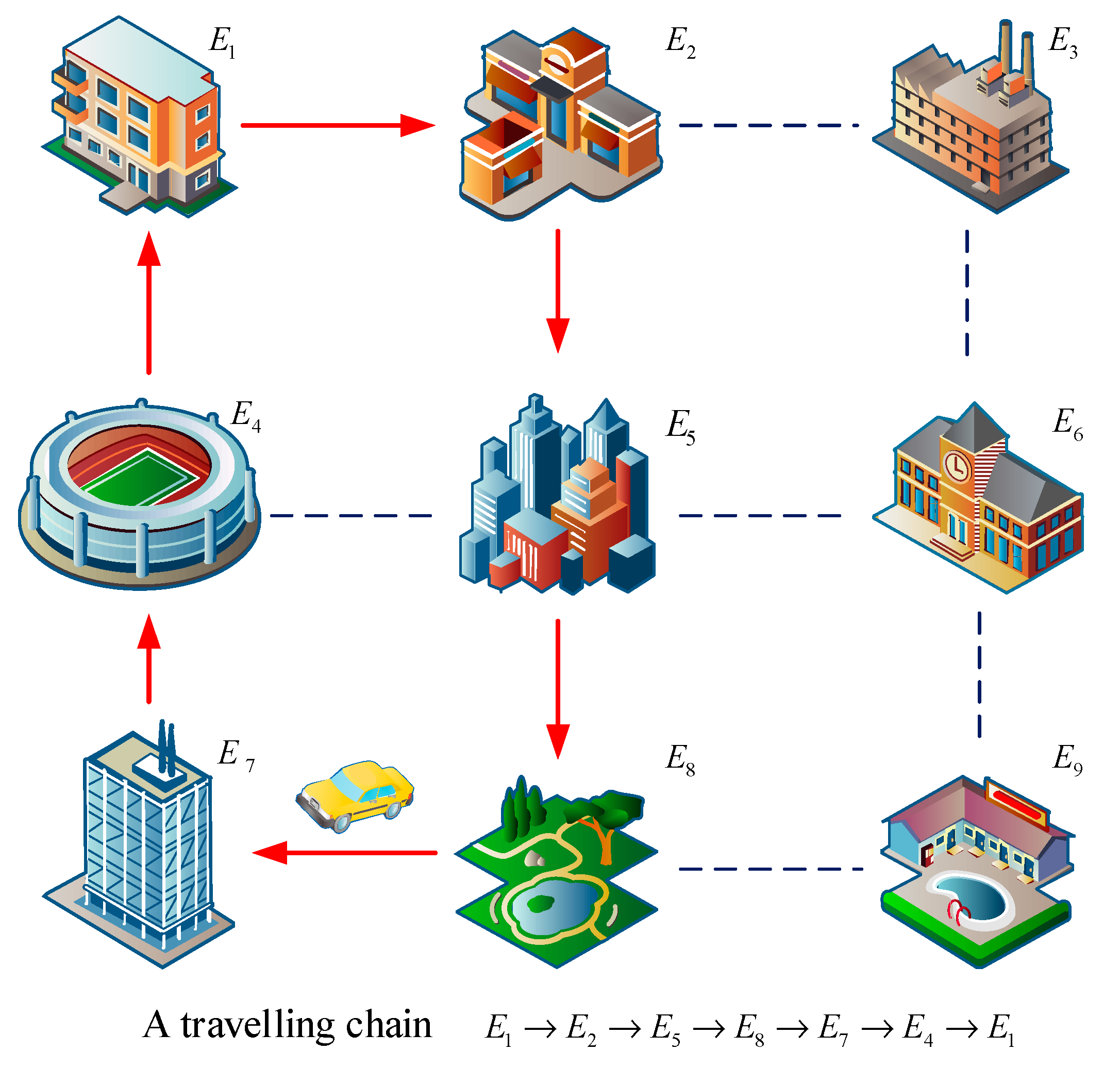
Figure 3.
Travel chain diagram.

Figure 4.
Electric vehicle charging load forecasting flow chart.

Figure 5.
Charging load curve for different functional areas.

Figure 6.
Charging load curve for different fast charge ratios.

Figure 7.
Optimized scheduling scheme for accessing EV.

Figure 8.
Optimized scheduling scheme for unconnected EV.


Table 1.
Electric vehicle charging interface parameters.
| Functional Areas | Charging Method | Charging Power/kW |
|---|---|---|
| Residential area | slow/fast | 3.2/37.1 |
| Work area | slow/fast | 5.9/58.5 |
| Business district | slow/fast | 5.2/46.4 |
Table 2.
Distributed power parameters.
| Power Type | Power/kW | Quantity |
|---|---|---|
| Wind turbines | 60 | 75 |
| Photovoltaic | 30 | 35 |
| Battery | 20 | 20 |
| EV | 20 | 50 |
Table 3.
Electricity price for each period of electricity purchased from the power grid.
| Electricity Price (¥/kW·h) | Period |
|---|---|
| 0.6 | 24:00–9:00 |
| 0.8 | 12:00–16:00/22:00–24:00 |
| 1.36 | 9:00–12:00/16:00–22:00 |
Table 4.
Demand response (DR) resource parameter.
| DR Resource | Response Capacity Maximum (kW) | Response Capacity Minimum (kW) | Compensation Price (¥/kW·h) |
|---|---|---|---|
| DR | 800 | 50 | 0.72 |
| EV | 400 | 20 | 0.8 |
Table 5.
Power generation costs of two optimized scheduling schemes.
| Schemes | Power Generation Cost (¥) | Reduction |
|---|---|---|
| Optimized scheduling scheme for accessing EV | 58394.2 | - |
| Optimized scheduling scheme for unconnected EV | 56753.3 | 2.81% |
© 2019 by the authors. Licensee MDPI, Basel, Switzerland. This article is an open access article distributed under the terms and conditions of the Creative Commons Attribution (CC BY) license (http://creativecommons.org/licenses/by/4.0/).
Share and Cite
MDPI and ACS Style
Li, F.; Dou, C.; Xu, S. Optimal Scheduling Strategy of Distribution Network Based on Electric Vehicle Forecasting. Electronics 2019, 8, 816. https://doi.org/10.3390/electronics8070816
AMA Style
Li F, Dou C, Xu S. Optimal Scheduling Strategy of Distribution Network Based on Electric Vehicle Forecasting. Electronics. 2019; 8(7):816. https://doi.org/10.3390/electronics8070816
Chicago/Turabian StyleLi, Fenglei, Chunxia Dou, and Shiyun Xu. 2019. "Optimal Scheduling Strategy of Distribution Network Based on Electric Vehicle Forecasting" Electronics 8, no. 7: 816. https://doi.org/10.3390/electronics8070816
Note that from the first issue of 2016, this journal uses article numbers instead of page numbers. See further details here.