Application of the Lyapunov Algorithm to Optimize the Control Strategy of Low-Voltage and High-Current Synchronous DC Generator Systems

Abstract

In the present study, a novel multiple three-phase low-voltage and high-current permanent magnet synchronous generation system is proposed, which has only half-turn coils per phase. The proposed system is composed of a generator and two confluence plates with 108 rectifier modules. The output can reach up to 10,000 A continuous DC power supply, which is suitable for the outdoors and non-commercial power supply. The application of the Lyapunov algorithm in the synchronous rectification control was optimized. A current sharing loop control was added to the closed-loop control to ensure a stable output voltage and the output current sharing of each rectifier module. Since the two control variables solved by the Lyapunov algorithm were coupled and the negative definite function of the Lyapunov algorithm could not be guaranteed in this system, a simple decoupling method was used to decouple the control variables. Compared to the conventional control, the proposed strategy highly improved the dynamic performance of the system. The effectiveness of the proposed strategy was verified by the simulation. The 5 V/10,000 A hardware experiment platform was built, which proved the feasibility and validity of the proposed strategy for a high-power generation system.

1. Introduction

Low-voltage and high-current generation systems with currents higher than 10,000 A are widely used in ships, electrolytic plating, and industrial fields. Considering the integration of motor and power electronics technology, the synchronous generation system has developed rapidly from high power density, high reliability, and high fault tolerance points of view [1]. In the present study, a three-phase rectifier module is used to generate direct current (DC) through a confluence plate, based on a permanent magnet synchronous motor with only half-turn coil per phase. In order to ensure that the integrated DC generation system generates high quality electrical power, the present study focuses on the control strategy of this system

The control strategy of three-phase rectifier circuits has been extensively studied by many researchers. Thomas A.F. first proposed the hysteresis current control; in [2,3] this control method was adopted in the current inner loop. It is also proven that the disadvantage of this method is that the switching frequency changes as the load current changes. In other words, this method cannot guarantee a fixed switching frequency in a power cycle. This causes additional stress on the switching device and reduces the service life of the device. Kalman proposed the dead-beat control theory, which is a control method based on circuit equations. In [4], an improved implementation of the deadbeat current controller was considered that is aimed at two purposes: The minimization of the small-signal response delay and the optimization of the large-signal step response. This method cancels the zero with the pole by using state feedback and configures another pole at the origin [5]. However, studies showed that this method has major drawbacks, including a high real-time requirement for calculating the pulse width and the sensitivity of system stability to the circuit parameters and weaknesses. Although the aforementioned drawbacks can be resolved by employing a complicated algorithm and a current observer, a large error will be generated. Zadeh L.A. proposed the fuzzy control based on fuzzy reasoning, which mimics the human mindset and controls a model where it is difficult to establish an accurate mathematical expression. In [6], a modified zero-voltage switching pulse width-modulation inverter with a digital signal processor-based proportional integral derivative-like fuzzy controller was implemented. The switches of the inverter achieved a soft-switching feature that largely reduced switching losses and improved the converting efficiency. The disadvantage of this control strategy is that it only relies on the experience and attempt to design the controller. There is no systematic method of analyzing and designing the controller. The cycle is long and the precision is low. Once the adaptive limit is exceeded, this method will no longer be applicable [7]. Tokuo Ohnishi proposed the direct power control method. The proposed control method indirectly controls the output current through the direct control of active and reactive power. Moreover, this method establishes the voltage and the current double closed-loop model, according to the AC voltage and instantaneous power to select the output state corresponding to the switch table. In [8], a direct power control using the natural switching surface was proposed; the proposed control considered the output voltage when selecting the switching states. Therefore, the proposed control does not need an outer voltage control loop and can highly improve the dynamic performance of the DC output voltage. The advantages of this method are the high-power factor, the high efficiency factor, and the ability to be used in a wide variety of applications [9,10]. However, due to the limitation of the current loop, it easily generates harmonic distortion in the input current, thereby reducing the power factor.

Lyapunov proposed the stability criterion control theory, which initially constructs a scalar energy-like function for the system and then designs the controller under the premise that the change in time of this function is negative [11]. This method was introduced into the rectifier control of a three-phase pulse with modulation (PWM) by Hasan K. [12]. He utilized the Lyapunov algorithm to control the three-phase rectifier system. This algorithm has the advantage that the system’s stability is not interfered with by large signals and is independent of circuit parameters. At present, the application of the Lyapunov algorithm to control PWM rectifiers is concentrated on grid voltage rectification [13,14] where there is a mutual coupling phenomenon between the obtained control variables, which cannot guarantee the long-term stable operation of the system. This study first proposes the application of the Lyapunov algorithm to a multiple three-phase permanent magnet in the synchronous generator system. It is expected that the system with the proposed control scheme can provide a reasonable transient response, unified power factor control, reduced harmonics on the AC side and an increase in the reliability of the generation system. In order to ensure the stable operation of the system, the proposed method decouples the control variables in a simple way.

2. Methods

2.1. Parallel Scheme of the Multiple Rectification Module

The studied high-current generation system is a new DC power generation system that realizes electromechanical energy conversion by using a multiple three-phase permanent magnet synchronous motor. The system directly generates low-ripple and high-intensity DC power through the combination of the modular rectification component and the high current confluence plate [15]. The advantages of this system are as the following:

• The phase voltage and the phase current can be reduced to generate low voltage and high power.
• The harmonic loss can be reduced to improve generator efficiency.
• Each phase is driven separately to improve the fault tolerance and the reliability of the system.
• Considering the special design of the confluence plate, the ripple of the output voltage is low when the system generates the high current [16]. Therefore, the output current can be used with no filtering for the majority of applications.

Figure 1 illustrates the designed model of the multiple three-phase permanent magnet synchronous high-current generation system. It indicates that the designed system is mainly composed of a permanent magnet synchronous generator with a half-turn coil for each phase and two confluence plates. Figure 1a describes the minimum cell which is composed of each winding and the leg of the bridge, and Figure 1b describes the five MOSFETs on each leg which are fixed on the heat sink. Moreover, Figure 1c shows a confluence plate that fixes the heat sink to be used as the output bus. In order to improve the heat-dissipation efficiency, the inside of the confluence plate is machined with a water-cooled passage. Figure 1d shows the overall model of the system containing the permanent magnet in the synchronous generator.

The generator rotor contains 6 pairs of magnetic poles and the stator core is internally opened with 54 slots. Each slot is embedded with a half-turn coil, containing the insulation as one phase, while the three-phase stator windings are placed at an electrical angle of 120°. It should be indicated that the two adjacent three-phase winding units differ from each other by an electrical angle of 2π/9. Moreover, each positive and negative confluence plate is composed of 54 MOSFET rectifier modules. The rectifier modules can be distributed along the circumference surface of the confluence plate as a stationary part of the synchronous generator. In order to simplify the analysis, only three rectifier modules were considered in the design and analysis. These modules correspond to the spaces of nine stator windings of the synchronous generator, which can form a 360° electrical angular space. The system is managed hierarchically, where the top layer is the management layer and the controller area network (CAN) bus transmits the current sharing information. The second layer of each control module analyzes the collected module voltage and compares it with current signals to generate the PWM control information to drive the switching device of the rectifier. The bottom layer is a three-phase PWM rectifier module, which is fixed at the bottom of the generator together with the confluence plate to generate high currents. Figure 2 shows the block diagram of the synchronous DC power generation system with the multi-phase permanent magnet.

The digital current sharing by the CAN bus can avoid the defects of the conventional master–slave control mode. This reduces the number of controllers and avoids the failure of the main control module not achieving the appropriate current sharing [17]. The CAN bus realizes the current sharing by means of competition where the module which generates the maximum current is determined as the main module and the corresponding maximum current is used as the reference current of the submodule. Even if the main module fails and shuts down, the other modules can continue to qualify as the main module in a competitive manner.

A modular rectifier improves system performance. First of all, the modular parallel connection is adopted in this rectification system, and the ripple of output is small, so that a rapid voltage adjustment method can be adopted without causing distortion of the input current, and the dynamic performance is good. Secondly, when the modules are connected in parallel to supply power to the load, even if a module fails, as long as it is removed from the parallel system in time, the load power supply can be ensured without interruption, further improving the reliability and flexibility of the power supply system. Finally, when powered by a parallel system, the power of each parallel module will be reduced, while the low power module can operate at a higher switching frequency, which can reduce the volume of the filter capacitor and increase the power density of the parallel system, which is very suitable for low- voltage and high-power systems.

2.2. Design of the Three-Phase Rectifier Controller, Based on the Lyapunov Algorithm

2.2.1. Mathematical Model of the Three-Phase Voltage Source PWM Rectifier in the d-q Synchronous Rotating Coordinate System

The state equation of the three-phase voltage source PWM rectifier is described by the unipolar binary logic switching function. When the coordinate transformation of the constant power is carried out, the mathematical models in the three-phase rotating coordinate system can be written as the following [18]:

$$L\frac{d{i}_d}{dt}=\omega L{i}_q-R{i}_d+e_d-v_o{p}_d$$

(1)

$$L\frac{d{i}_q}{dt}=-\omega L{i}_d-R{i}_q+e_q-v_o{p}_q$$

(2)

$$C\frac{d{v}_o}{dt}=\frac{3}{2}(P_d{i}_d+P_q{i}_q)-i_o$$

(3)

where v_o, i_o, L and C denote the output voltage, module current, AC side inductance, and the DC side filter capacitance, respectively. On the other hand, ω is the angular frequency. Furthermore, p_d and p_q are voltage modulation ratios on d and q axes, respectively. Finally, i_d, i_q, e_d, e_q denote the currents and voltages of the network side in the synchronous rotating coordinate system, respectively.

2.2.2. Lyapunov Control Algorithm

Studies showed that the hysteresis current control, the deadbeat control and the fuzzy control methods yield various advantages and disadvantages [19,20,21] from different points of view, including the circuit complexity, switching frequency, and the transient state. A common disadvantage of these methods is that system stability cannot be guaranteed under large signal interference. Since the system generates high current, the voltage produces large fluctuations when subjected to large signal interference, which affects the normal operation of the system. In [9], the controller is derived based on direct Lyapunov stability theory in order to calculate proper switching functions, Setting up the controller with this switch function, the results show the appropriate performance of the proposed controllers during both steady-state and transient dynamic conditions. Considering the abovementioned challenge, a nonlinear control strategy based on the Lyapunov direct method [22,23] is proposed to strictly guarantee the global asymptotic stability of the rectifier. The purpose of this control strategy is to make the output voltage close to the reference voltage (V_r) and provide a unity power factor with a nearly sinusoidal input current. When the system is controlled by the Lyapunov algorithm, it is necessary to construct an “energy-like” function for the system, and then design the controller under the premise of ensuring that the function is always negative. Finally, establishing the Lyapunov function based on the quantitative correlation of the energy storage of the inductor and the capacitor. Suppose that the Lyapunov function is a positive definite function, while its derivative is negative definite function. When x tends to infinity in any direction, V(x) also approaches infinity. The equilibrium point at the origin is globally asymptotically stable.

Letting the operating point of the system energy stability be the equilibrium point, we define a positive definite Lyapunov function as the following:

$$V(\overline{x})=\frac{3}{2}L{x}_1^2+\frac{3}{2}L{x}_2^2+C{x}_3^2$$

(4)

where x₁, x₂ and x₃ are system state variables defined as the following:

$$\{\begin{array}{l}{x}_1=i_d-i_{d0}\\ x_2=i_q\\ x_3=V_r-v_o+k(I_r-i_o)\end{array}$$

(5)

where V_r, I_r, k and i_d0 denote the reference voltage, reference current, proportional coefficient, and the steady value of i_d, respectively. It should be indicated that the reference current is maximum current in the multiple rectification. The derivative of the Lyapunov function is

$$V^{\prime }(\overline{x})=3x_{1}L{x}_1^{\prime }+3x_{2}L{x}_2^{\prime }+2x_{3}C{x}_3^{\prime }$$

(6)

According to the first Lyapunov stability theorem, when the Lyapunov derivative is negative, the system is stable in the equilibrium point. Let i_q = 0 to ensure unit power factor, when the system is stable, the parameter values of the equilibrium point are as follows:

$$\{\begin{array}{l}{v}_o=V_r\\ i_o=I_r\\ i_d=i_{d0}\\ e_d=E_m\\ i_q=0\\ p_d=p_{d0}\\ p_q=p_{q0}\end{array}$$

(7)

where p_d0 and p_q0 are the control variables when the system is stable and E_m is the amplitude of the phase voltage.

After substituting Equation (7) into Equations (1)–(3) and a simple manipulation, the following expressions are obtained:

$$p_{d0}=(E_m-R{i}_{d0})/V_r$$

(8)

$$p_{q0}=-\omega L{i}_{d0}/V_r$$

(9)

$$i_o=\frac{3}{2V_r}(E_m{i}_{d0}-R{i}_{d0}^2)$$

(10)

$$i_{d0}=\frac{1}{2}\left\{\frac{E_m}{R}\pm {\left[{\left(\frac{E_m}{R}\right)}^2-\left(\frac{8V_r{i}_o}{3R}\right)\right]}^{\frac{1}{2}}\right\}$$

(11)

Assuming that the system is disturbed, the variations of voltage-space vector modulation ratio on d and q axes are Δp_d and Δp_q, respectively. Then the actual modulation ratios of output voltage can be obtained as the following:

$$p_d=p_{d0}+\Delta p_d$$

(12)

$$p_q=p_{q0}+\Delta p_q$$

(13)

Substitute Equations (5), (8) and (12) into Equation (1) results in the following equation:

$$\begin{array}{ll}L{x}_1^{\prime }=& \omega L{x}_2-V_r\Delta p_d-\frac{\left(E_m-R{i}_{d0}\right)\left[x_3+k\left(I_r-i_o\right)\right]}{V_r}\\ & -\left[x_3+k\left(I_r-i_o\right)\right]\Delta p_d-R{x}_1\end{array}$$

(14)

Similarly, Equations (5), (9) and (13) are applied to Equation (2) so that the following equation is obtained:

$$\begin{array}{ll}L{x}_2^{\prime }=& -\omega L{x}_1-V_r\Delta p_q-\frac{\omega L{i}_{d0}\left[x_3+k\left(I_r-i_o\right)\right]}{V_r}\\ & -\left[x_3+k\left(I_r-i_o\right)\right]\Delta p_q-R{x}_2\end{array}$$

(15)

Moreover, Equations (5), (10), (12) and (13) are implemented into Equation (3) to obtain the following equation:

$$\begin{array}{ll}C{x}_3^{\prime }=& \frac{3}{2}[\frac{\left(E_m-R{i}_{d0}\right)}{V_r}{x}_1+i_{d0}\Delta p_d+\Delta p_d{x}_1\\ & -\frac{\omega L{i}_{d0}}{V_r}{x}_2+\Delta p_q{x}_2]\end{array}$$

(16)

Substituting Equations (10) and (14)–(16) into Equation (6) yields the following equation:

$$\begin{array}{ll}{V}^{\prime }\left(\overline{x}\right)=& -3\left\{\left[V_r+k\left(I_r-i_o\right)\right]x_1-i_{d0}{x}_3\right\}\Delta p_d\\ & -3x_2\left[V_r+k\left(I_r-i_o\right)\right]\Delta p_q-3R\left(x_1^2+x_2^2\right)\end{array}$$

(17)

When the following conditions are met, the Lyapunov derivative along any of the trajectories of the system is negative:

$$\Delta p_d=\gamma \left\{\left[V_r+k\left(I_r-i_o\right)\right]x_1-i_{d0}{x}_3\right\},\gamma >0$$

(18)

$$\Delta p_q=\beta x_2\left[V_r+k\left(I_r-i_o\right)\right],\beta >0$$

(19)

where β and γ are arbitrary real constants.

2.2.3. Saturation Constraint and Decoupling Control Variables

The switching state of the rectifier is determined by the space vector pulse width modulation method (SVPWM) [24]. In order to ensure that the rectifier is in sinusoidal steady-state operation and the switching function is not saturated, the following conditions must be met:

$${\left(p_{d0}+\Delta p_d\right)}^2+{\left(p_{q0}+\Delta p_q\right)}^2\le \frac{4}{3}$$

(20)

The control variables, which satisfy the SVPWM are obtained from Equation (20) as the following:

$${\left(\Delta p_d\right)}_{m1}=\frac{2\left(p_{d0}+\Delta p_d\right)}{\sqrt{3\left[{\left(p_{d0}+\Delta p_d\right)}^2+{\left(p_{q0}+\Delta p_q\right)}^2\right]}}-p_{d0}$$

(21)

$${\left(\Delta p_q\right)}_{m1}=\frac{2\left(p_{q0}+\Delta p_q\right)}{\sqrt{3\left[{\left(p_{d0}+\Delta p_d\right)}^2+{\left(p_{q0}+\Delta p_q\right)}^2\right]}}-p_{q0}$$

(22)

The two control variables (Δp_d)_m1 and (Δp_q)_m1 are mutual coupling and non-linear variables, which cannot guarantee a negative Lyapunov derivative. Therefore, it is necessary to decouple the control variables. Assuming that the system is controlled by p_q, (i.e., p_d = 0), then the range of Δp_q can be written as

$$-\left(p_{q0m}+p_{q0}\right)\le \Delta p_q\le p_{q0m}-p_{q0}$$

(23)

P_q0m represents the maximum possible steady-state value that p_q can take for the maximum DC load current. Similarly, the range of Δp_d can be written as

$$-\left(p_{d0m}+p_{d0}\right)\le \Delta p_d\le p_{d0m}-p_{d0}$$

(24)

P_d0m is the maximum steady-state value of p_d, which can be calculated by Equation (25) as the following:

$$p_{d0m}=\sqrt{\frac{4}{3}-p^2{}_{q0m}}$$

(25)

Therefore, the control variables are rewritten as the following:

$${\left(\Delta p_d\right)}_{m2}=\{\begin{array}{ll}-\left(p_{d0m}+p_{d0}\right)& \gamma \left\{\left[V_r+k\left(I_r-i_o\right)\right]x_1-i_{d0}{x}_3\right\}<-\left(p_{d0m}+p_{d0}\right)\\ \gamma \left\{\left[V_r+k\left(I_r-i_o\right)x_1-i_{d0}{x}_3\right]\right\}& -\left(p_{d0m}+p_{d0}\right)\le \gamma \left\{\left[V_r+k\left(I_r-i_o\right)\right]x_1-i_{d0}{x}_3\right\}\le \left(p_{d0m}-p_{d0}\right)\\ p_{d0m}-p_{d0}& \gamma \left\{\left[V_r+k\left(I_r-i_o\right)x_1-i_{d0}{x}_3\right]\right\}>\left(p_{d0m}-p_{d0}\right)\end{array}$$

(26)

$${\left(\Delta p_q\right)}_{m_2}=\{\begin{array}{ll}-\left(p_{q0m}+p_{q0}\right)& \beta {\mathrm{x}}_2\left[V_r+k\left(I_r-i_o\right)\right]<-\left(p_{q0m}+p_{q0}\right)\\ \beta {\mathrm{x}}_2\left[V_r+k\left(I_r-i_o\right)\right]& -\left(p_{q0m}+p_{q0}\right)\le \beta {\mathrm{x}}_2\left[V_r+k\left(I_r-i_o\right)\right]\le p_{q0m}-p_{q0}\\ p_{q0m}-p_{q0}& \beta {\mathrm{x}}_2\left[V_r+k\left(I_r-i_o\right)\right]>p_{q0m}-p_{q0}\end{array}$$

(27)

Figure 3 illustrates that the voltage vector of the rotation is in the rectangular area of the dotted round line. Under the control rules of Equations (26) and (27), the Lyapunov derivative is a negative definite function. Meanwhile, the stability of the system is independent of the circuit parameters.

2.2.4. SVPWM Algorithm

The final voltage modulation ratio p_d, p_q is as follows:

$$p_d=p_{d0}+{(\Delta p_d)}_{m2}$$

(28)

$$p_d=p_{d0}+{(\Delta p_d)}_{m2}$$

(29)

Then the inverse Park transformation on p_d, p_q, is as shown in Figure 4.

Here, p_d and p_q are inversely transformed into U_α and U_β, and the electrical angle θ is taken as the angle. Then, p_d and p_q are respectively vector-decomposed, and the voltage components on the α-axis and the β-axis are calculated as follows:

$$U_{\alpha }=p_d\ast \cos \theta -p_q\ast \sin \theta$$

(30)

$$U_{\beta }=p_q\ast \cos \theta -p_d\ast \sin \theta$$

(31)

Then, we apply the inverse Park transformation on U_α, U_β, converting the target voltage vector U_out into a balanced three-phase voltage vector U_a, U_b, U_c, as follows:

$$\{\begin{array}{l}{U}_{\mathrm{a}}=U_{\beta }\\ U_b=\frac{-U_{\beta }+\sqrt{3}{U}_{\alpha }}{2}\\ U_c=\frac{-U_{\beta }-\sqrt{3}{U}_{\alpha }}{2}\end{array}$$

(32)

We can determine the sector of U_out by defining variables a, b, and c according to Equation (33).

$$N=4a+2b+c$$

(33)

The correspondence between the value of N and the sector is as

Table 1. The sector.

N	3	1	5	4	6	2
Sector	Ⅰ	Ⅱ	Ⅲ	Ⅳ	Ⅴ	Ⅵ

:

In Figure 5, the target voltage vector U_out is analyzed in the I sector, TS is the PWM carrier period, T₀, T₇ is zero voltage vector time, T₄ is the U₄ time, T₆ is the U₆ time, and θ is electrical angle of the U_out. The following relationships can be obtained from Figure 5.

$$\left[\begin{array}{l}{U}_{\alpha }\\ U_{\beta }\end{array}\right]T_s=U_{out}\left[\begin{array}{l}\cos \theta \\ \sin \theta \end{array}\right]T_s=\frac{2}{3}{U}_{dc}\left[\begin{array}{l}1\\ 0\end{array}\right]T_4+\frac{2}{3}{U}_{dc}\left[\begin{array}{l}\cos \frac{\pi }{3}\\ \sin \frac{\pi }{3}\end{array}\right]T_6$$

(34)

From Equation (34), there are

$$\{\begin{array}{l}{T}_4=\frac{\sqrt{3}{T}_s}{U_{dc}}(\frac{\sqrt{3}}{2}{U}_{\alpha }-\frac{U_{\beta }}{2})\\ T_6=\frac{\sqrt{3}{T}_s}{U_{dc}}{U}_{\beta }\\ T_0=T_7=\frac{1}{2}(T_s-T_4-T_6)\end{array}$$

(35)

In the same way, the time of each vector of U_out in other sectors is obtained. The result is shown in

Table 2. The time of the basic space vector of each sector.

Sector Ⅰ	$T_4=\frac{\sqrt{3}{T}_s}{U_{dc}}(\frac{\sqrt{3}}{2}{U}_{\alpha }-\frac{U_{\beta }}{2})=K{U}_b$ $T_6=\frac{\sqrt{3}{T}_s}{U_{dc}}{U}_{\beta }=K{U}_a$ $T_0=T_7=(T_s-T_4-T_6)/2$	Sector Ⅱ	$T_6=\frac{\sqrt{3}{T}_s}{U_{dc}}(\frac{\sqrt{3}}{2}{U}_{\alpha }+\frac{U_{\beta }}{2})=K{U}_c$ $T_2=-\frac{\sqrt{3}{T}_s}{U_{dc}}(\frac{\sqrt{3}}{2}{U}_{\alpha }-\frac{U_{\beta }}{2})=-K{U}_b$ $T_0=T_7=(T_s-T_2-T_6)/2$
Sector Ⅲ	$T_2=\frac{\sqrt{3}{T}_s}{U_{dc}}{U}_{\beta }=K{U}_a$ $T_3=\frac{\sqrt{3}{T}_s}{U_{dc}}(-\frac{\sqrt{3}}{2}{U}_{\alpha }-\frac{U_{\beta }}{2})=K{U}_c$ $T_0=T_7=(T_s-T_2-T_3)/2$	Sector Ⅳ	$T_3=\frac{\sqrt{3}{T}_s}{U_{dc}}(-\frac{\sqrt{3}}{2}{U}_{\alpha }+\frac{U_{\beta }}{2})=-K{U}_b$ $T_1=-\frac{\sqrt{3}{T}_s}{U_{dc}}{U}_{\beta }=-K{U}_a$ $T_0=T_7=(T_s-T_1-T_3)/2$
Sector Ⅴ	$T_1=\frac{\sqrt{3}{T}_s}{U_{dc}}(-\frac{\sqrt{3}}{2}{U}_{\alpha }-\frac{U_{\beta }}{2})=K{U}_c$ $T_5=\frac{\sqrt{3}{T}_s}{U_{dc}}(\frac{\sqrt{3}}{2}{U}_{\alpha }-\frac{U_{\beta }}{2})=K{U}_b$ $T_0=T_7=(T_s-T_1-T_5)/2$	Sector Ⅵ	$T_5=-\frac{\sqrt{3}{T}_s}{U_{dc}}{U}_{\beta }=-K{U}_a$ $T_4=\frac{\sqrt{3}{T}_s}{U_{dc}}(\frac{\sqrt{3}}{2}{U}_{\alpha }+\frac{U_{\beta }}{2})=-K{U}_c$ $T_0=T_7=(T_s-T_4-T_5)/2$

, where the $K=\sqrt{3}{T}_s/U_{dc}$.

3. Results and Discussion

In order to verify the efficiency of the proposed control strategy compared to that of conventional methods, the direct power control algorithm [25,26], dead-Beat control algorithm, which are widely used in three-phase PWM rectifier systems, were selected in the present study. The studied parameters included the dynamic performance, reliability and independency of the large signal interference for the control of the new synchronous generation system with a multiple three-phase permanent magnet. Figure 6 shows the block diagram of the control system. Moreover, Figure 7 illustrates the three-module parallel simulation model. The simulation parameters of the three-phase PWM rectifier are as

Table 3. Electrical parameters power circuit.

Parameter	Value
Line to line ac voltage, E	4.2 V
Source voltage frequency, f	50 Hz
Switching frequency	20 kHz
dc-bus capacitor, C	2200 uF
dc-bus voltage, vdc	5 V
Sample frequency	50 μs
Resistance of smoothing inductor, R	0.56 Ω
Inductance of smoothing inductor, L	1.5 mH
Load resistance RL	32 Ω

:

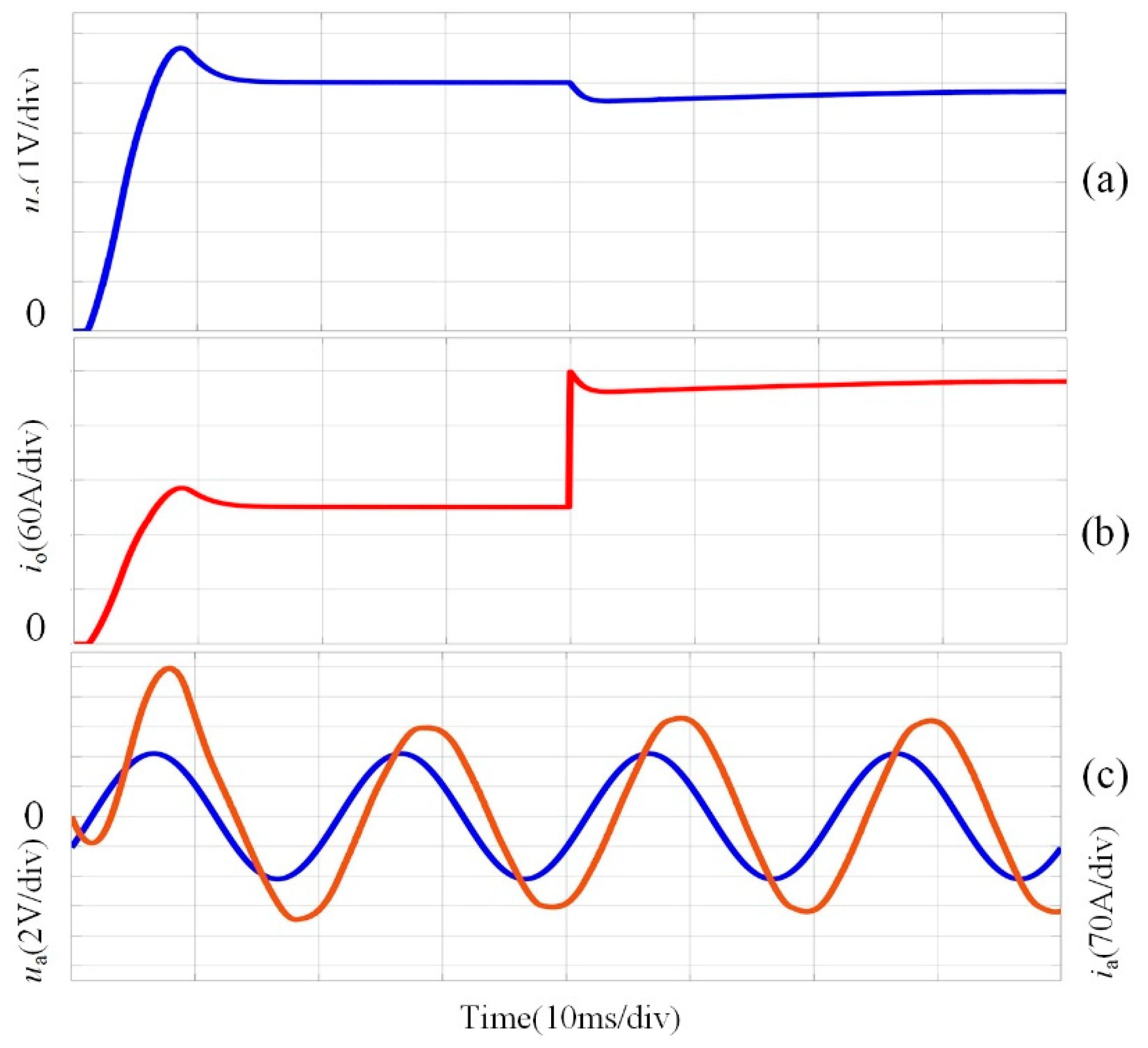
3.1. The Control Based on the Lyapunov Algorithm

Figure 8 shows the output voltage, current and AC side A-phase voltage and current response curves of the system during the load is 32 Ω. Figure 8a indicates that during the power-on process, the system voltage overshoot is 10%, the system reaches the steady state in 0.02 s and the output voltage is 5 V. Moreover, Figure 8b shows that the output current is 150A. Figure 8c shows the waves of the input. It is observed that the current fluctuates before 0.02 s and there is a short overshoot. Meanwhile, the system is stable after 0.02 s and achieves unit power factor. Figure 8d shows the spectrum of the A-phase current. It is found that the A-phase current contains low harmonics, where the total harmonic distortion (THD) rate is THD = 1.02%.

Figure 9 shows the output voltage, current and AC side of the A-phase voltage and current response curves of the system when the load suddenly changes from 32 to 16 Ω. Figure 9a illustrates that the system is stable in the 0.02 s, the load is halved in 0.03 s and the voltage changes to about 0.2 V. Moreover, Figure 9b shows that the system reaches the steady state after 0.02 s and the output current is doubled to 300 A. Figure 9c shows that the phase voltage and current briefly fluctuate and they re-implement the unit power factor.

3.2. The Control Based on the Direct Power Algorithm

Figure 10 shows the voltage, current and AC side of the A-phase voltage and current response curves of the system during the control of the direct power algorithm. Figure 10a shows that the system is stable at 0.02 s, while the voltage drops when the load is halved at 0.04 s. The system adjusts to a new steady state after 0.03 s and the output voltage drops to 4.8 V, which is less than the reference voltage. Figure 10b shows the output current wave. It is observed that the current increases rapidly and reaches 148 A. Furthermore, Figure 10c shows the AC side of the A-phase voltage and current waveforms. It is found that the current increases after 0.04 s, while the unit power factor is still not guaranteed.

3.3. The Control Based on the No Beat Control Algorithm

Figure 11 is the waveform with no beat control. It can be seen that the voltage overshoot is 20%, the system reaches the steady state in 0.03 s when the load resistance suddenly changes from 32 Ω to 16 Ω at 0.06 s, the voltage change is about 0.8 V, and the steady state is restored after 0.03 s. The output current is doubled to 300 A, and the phase A voltage and current achieve a unit power factor after a short period of fluctuation.

Figure 12 shows output current waveforms of the three-module system in parallel mode. Each rectifier module is controlled by the autonomous current sharing. In all of the parallel modules, the module with the highest output current automatically becomes the main module through the current sampling and the current sharing control bus sends reference current information to other modules to achieve the current sharing. The simulation results indicate that after the current sharing control, each module can generate a stable current of 300 A.

It is concluded from the abovementioned comparisons that the voltage overshoot is 10%, 14%, and 20% when the system is controlled by the Lyapunov algorithm, direct power algorithm, and dead-beat algorithm, respectively. Moreover, when the load varies, the Lyapunov algorithm restores the steady state after 0.02 s adjustment, while the output voltage is 5 V. On the other hand, the direct power algorithm reaches a new steady state after 0.03 s, while the output voltage is 4.8 V. In other words, the steady state voltage of the Lyapunov algorithm is slightly higher than that of the direct power algorithm. Meanwhile, the voltage drops and produces 4% error. When the dead-beat algorithm is used as control, the load changes and the system reaches a new steady state after 0.03 s. Here, the restoring time of steady state is longer than that of Lyapunov algorithm. On the AC side, the Lyapunov control algorithm can realize the unit power factor and the overshoot of the current before and after the load mutation is low. However, when the direct power control is adopted, the phase difference of the single-phase voltage and current exists all the time. The unit power factor cannot be realized by the direct power control algorithm because it needs to estimate the instantaneous reactive power and then estimate the voltage vector of the AC side. Since the AC current is large, when the current transient tracking index is satisfied, the AC side inductance is limited. The inductance affects the accuracy of the estimation of instantaneous reactive power, which leads to the phase difference between the voltage and current on the AC side. Thus, the unit power factor cannot be realized.

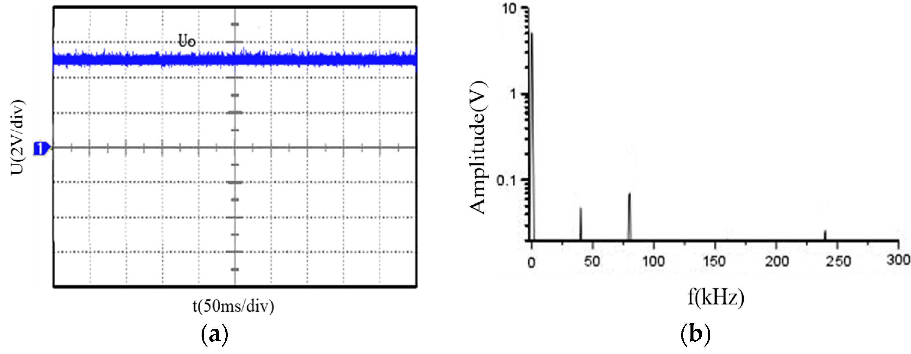
3.4. Verification of the Experimental Result

The main electrical parameters of the power circuit and control data, used in the implementation tests, are given in Table 3. The development of control algorithms was performed and simulated with Matlab/Simulink and the real-time implementation with a Texas Instrument digital signal processor (DSP) board (TMS320F28335). Each three-phase winding was used as an independent module. Each module, using a 32-bit DSP28335 processor, operated at a frequency of 150 MHz, with a bandwidth of 600 Mbps and a single precision floating-point-unit (FPU). The current sharing control was realized by CAN bus among the controllers, which improved the independence and reduced the interference of the modules, so the traditional fixed-point MCU would affect the result of algorithm processing. The control strategy can be used in the mainstream 32-bit floating-point microprocessor and 10-bit or more AD sampling. Figure 13 shows the experimental platform, which is the setup for experimental verification. This setup was used to verify the validity of the proposed Lyapunov control algorithm. When carrying out a load test, the setup can adjust the resistor box terminal to provide 10–1000 mΩ.

Figure 14 shows the experiment waves of the output current and the three-phase AC current waveforms when a single rectifier module is in operation. When the load suddenly changed from 32 to 16 Ω at 0.04 s, as can be seen, the system reached the steady state in less than 0.02 s, their steady-state performances were both quite good. The proposed control can highly improve the dynamic performance of the DC output current with a shorter transition time. It is consistent with the simulation results.

Figure 15 shows the experiment waves of the output voltage and the corresponding frequency spectrum when a single rectifier module is in operation. The logarithmic uniform distribution is used to facilitate the comparison of the longitudinal axis. The diagram shows that the output voltage of the rectifier module is stable. The amplitude of the voltage is 5 V when the main frequency is 0 Hz, and the maximum value of the ripple of each frequency does not exceed 0.06 V, which meets the requirements of the DC output.

Figure 16 shows the experiment waves of the output current and the corresponding spectrum when a single rectifier module is in operation. The vertical axis is logarithmically and uniformly distributed. Moreover, the unit ratio is 100 A. When the main wave of the output current is stable, the main frequency is still 0 Hz, which conforms to DC characteristics. Although there is a certain amplitude in other frequency bands, none of them exceeds 3 A.

Figure 17 shows the waveforms’ output voltage when the system load increases and decreases suddenly. The diagram illustrates that when the load changes, the output external characteristics of the rectifier module of the generation system changes, under the condition of the same duty cycle. This may be attributed to the internal resistance inside the device. The output voltage in the diagram can be quickly restored to a stable state without overshooting, which proves that the dynamic control performance of the Lyapunov algorithm is superior over the conventional methods.

Figure 18 and Figure 19 present the current waveforms of the paralleling system when the light load switches to the heavy load, and vice versa. They indicate that the current variation and adjustment times are different between module 1 and 2. This originates from the two modules within the inherent relationship between different parameters and their corresponding master–slave structure, in which the regulating speed of the submodule is slower than that of the main module. Meanwhile, the control process contains the vibration. However, the two modules can quickly achieve stable output and current sharing, which proves the better dynamic response of digital current sharing, compared to the conventional methods.

4. Conclusions

Based on the current situation that a low-voltage high-current generation system focuses mainly on rectifying the voltage of the power grid, the present study proposes a synchronous generator system with a multiple three-phase permanent magnet, which is controlled by the Lyapunov algorithm. Through analysis, there is a problem of mutual coupling between the control variables. To solve this problem, a simple decoupling method was adopted. By decoupling, the Lyapunov derivative of the system is always negative, thus ensuring the stability of the system. Since the direct power control method and dead-beat algorithm are widely used, in this paper, these two methods were used to compare the performance. The simulation results show that when the Lyapunov algorithm is utilized for the synchronous generator system with a multiple three-phase permanent magnet, the system has low voltage overshoot, and reasonable dynamic and static performance. It is found that system stability is not disturbed by large signals and has reasonable performance for the unit power factor. The experimental results are consistent with the simulation, which proves that the control strategy is an effective and reliable control scheme.

References

1. Kassakian, J.G.; Jahns, T.M. Evolving and Emerging Applications of Power Electronics in Systems. IEEE J. Emerg. Sel. Top. Power Electron. 2013, 1, 47–58. [Google Scholar] [CrossRef]
2. Mohseni, M.; Islam, S.M. A New Vector-Based Hysteresis Current Control Scheme for Three-Phase PWM Voltage-Source Inverters. IEEE Trans. Power Electron. 2010, 25, 2299–2309. [Google Scholar] [CrossRef]
3. Du, J.; Zhao, H.; Zheng, T.Q. Study on a switching-pattern hysteresis current control method based on zero voltage vector used in three-phase PWM converter. IET Power Electron. 2017, 10, 2190–2198. [Google Scholar] [CrossRef]
4. Buso, S.; Tommaso, C.G.; Danilo, I.B. Dead-Beat Current Controller for Voltage-Source Converters with Improved Large-Signal Response. IEEE Trans. Ind. Appl. 2016, 52, 1588–1596. [Google Scholar] [CrossRef]
5. Cheng, C.W.; Nian, H.; Wang, X.H.; Sun, D. Dead-beat predictive direct power control of voltage source inverters with optimised switching patterns. IET Power Electron. 2017, 10, 1438–1451. [Google Scholar] [CrossRef]
6. Tao, C.-W.; Wang, C.-M.; Chang, C.-W. A Design of a DC–AC Inverter Using a Modified ZVS-PWM Auxiliary Commutation Pole and a DSP-Based PID-Like Fuzzy Control. IEEE Trans. Ind. Electron. 2016, 63, 397–405. [Google Scholar] [CrossRef]
7. Cecati, C.; Dell’Aquila, A.; Liserre, M.; Ometto, A. A fuzzy-logic-based controller for active rectifier. IEEE Trans. Ind. Appl. 2003, 39, 105–112. [Google Scholar] [CrossRef]
8. Ge, J.; Zhao, Z.; Yuan, L.; Lü, T.; He, F. Direct Power Control Based on Natural Switching Surface for Three-Phase PWM Rectifiers. IEEE Trans. Power Electron. 2015, 30, 2918–2922. [Google Scholar] [CrossRef]
9. Bouafia, A.; Krim, F.; Gaubert, J.-P. Fuzzy-Logic-Based Switching State Selection for Direct Power Control of Three-Phase PWM Rectifier. IEEE Trans. Ind. Electron. 2009, 56, 1984–1992. [Google Scholar] [CrossRef]
10. Malinowski, M.; Kaźmierkowski, M.; Hansen, S.; Blaabjerg, F.; Marques, G. Virtual-flux-based direct power control of three-phase PWM rectifiers. IEEE Trans. Ind. Appl. 2001, 37, 1019–1027. [Google Scholar] [CrossRef]
11. Li, H.; Wang, Y. Lyapunov-Based Stability and Construction of Lyapunov Functions for Boolean Networks. SIAM J. Control Optim. 2017, 55, 3437–3457. [Google Scholar] [CrossRef]
12. Hasan, K.; Osman, K. Lyapunov based control for three-phase PWM AC/DC voltage source converters. IEEE Trans. Power Electron. 1998, 13, 801–813. [Google Scholar]
13. Hadi, H.K.; Mahdi, B.; Ali, A.K. Direct-Lyapunov-based control scheme for voltage regulation in a three-phase islanded microgrid with renewable energy sources. Energies 2018, 11, 1161. [Google Scholar]
14. Arkadiusz, L.; Zbigniew, K.; Haitham, A.R. Space-vector pulse width modulation for three-level NPC converter with the neutral point voltage control. IEEE Trans. Ind. Electron. 2011, 58, 5076–5086. [Google Scholar]
15. Gu, Y.L.; Huang, G.S.; Zhang, J.F. A synchronous rectifier driving circuit for modules in parallel. Proc. CSEE 2005, 4, 25–29. [Google Scholar]
16. Mohamed, A. Harmonic elimination in three-phase voltage source inverters by particle swarm optimization. JEET 2011, 6, 334–341. [Google Scholar]
17. Lin, B.-R. Analysis of a DC Converter with Low Primary Current Loss and Balance Voltage and Current. Electronics 2019, 8, 439. [Google Scholar] [CrossRef]
18. Song, Z.F.; Tian, Y.J.; Yan, Z.; Chen, Z. Direct Power Control for Three-Phase Two-Level Voltage-Source Rectifiers Based on Extended-State Observation. IEEE Trans. Ind. Electron. 2016, 63, 4593–4603. [Google Scholar] [CrossRef]
19. Hang, L.; Liu, S.; Yan, G.; Qu, B.; Lu, Z.-Y. An Improved Deadbeat Scheme with Fuzzy Controller for the Grid-side Three-Phase PWM Boost Rectifier. IEEE Trans. Power Electron. 2011, 26, 1184–1191. [Google Scholar] [CrossRef]
20. Cheng, Q.M.; Cheng, Y.M.; Xue, Y. A summary of current control methods for three-phase voltage-source PWM rectifiers. Power Syst. Prot. Control 2012, 40, 145–155. [Google Scholar]
21. Qiu, X.-D.; Jung, Y.-G.; Lim, Y.-C. Three-Phase Z-Source PWM Rectifier Based on the DC Voltage Fuzzy Control. Trans. Korean Inst. Power Electron. 2013, 18, 466–476. [Google Scholar] [CrossRef] [Green Version]
22. Kwak, S.; Yoo, S.-J.; Park, J. Finite control set predictive control based on Lyapunov function for three-phase voltage source inverters. IET Power Electron. 2014, 7, 2726–2732. [Google Scholar] [CrossRef]
23. Abdul, M.D.; Tey, K.S.; Saad, M.; Mutsuo, N. Lyapunov law based on model predictive control scheme for grid connected three phase three level neutral point clamped inverter. In Proceedings of the 3rd International Future Energy Electronics Conference and ECCE Asia, Kaohsiung, Taiwan, 4–7 June 2017; pp. 512–516. [Google Scholar]
24. Feng, Y.L.; Zhang, C.N. Core loss analysis of interior permanent magnet synchronous machines under SVPWM excitation with considering saturation. Energies 2017, 10, 1716. [Google Scholar] [CrossRef]
25. Vazquez, S.; Sanchez, J.; Carrasco, J.; Leon, J.I.; Galvan, E. A Model-Based Direct Power Control for Three-Phase Power Converters. IEEE Trans. Ind. Electron. 2008, 55, 1647–1657. [Google Scholar] [CrossRef]
26. Wang, J.H.; Li, H.D.; Wang, L.M. Direct power control system of three phase boost type PWM rectifiers. Proc. CSEE 2006, 26, 54–60. [Google Scholar]
Figure 1. Schematic models of the rectifier module and the power generation system: (a) A leg of bridge; (b) heat sink; (c) schematic of the confluence plate; (d) schematic model of a large DC power generation system.
Electronics 08 00871 g001
Figure 2. The block diagram of the synchronous DC power generation system with the multi-phase permanent magnet.
Electronics 08 00871 g002
Figure 3. Modified control vector area.
Electronics 08 00871 g003
Figure 4. Coordinate transformation.
Electronics 08 00871 g004
Figure 5. I sector.
Electronics 08 00871 g005
Figure 6. System diagram of the single module control of the space vector pulse width modulation method (SVPWM) rectifier.
Electronics 08 00871 g006
Figure 7. The three-module parallel simulation model: (a) The main circuit model of a three-module system during the parallel simulation; (b) control loop model of a three-module system during the parallel simulation.
Electronics 08 00871 g007
Figure 8. Simulation waves of the Lyapunov control: (a) Steady-state voltage wave; (b) steady-state current wave; (c) A-phase voltage and current waves; (d) A-phase current spectrum.
Electronics 08 00871 g008aElectronics 08 00871 g008b
Figure 9. Simulation waves of the disturbed Lyapunov control: (a) Voltage wave; (b) Current wave; (c) A-phase voltage and current waves. (d) three-phase AC current waveform.
Electronics 08 00871 g009
Figure 10. Simulation waves of the disturbed direct power control: (a) Voltage wave; (b) current wave; (c) A-phase voltage and current waves.
Electronics 08 00871 g010
Figure 11. Simulation waves of the no beat control algorithm: (a) Voltage wave; (b) current wave; (c) A-phase voltage and current waves.
Electronics 08 00871 g011
Figure 12. Output current waveform of the three modules in parallel mode.
Electronics 08 00871 g012
Figure 13. Large current load experiment of the integrated DC output system: (a) Experimental platform; (b) load experiment; (c) the schematic of the synchronous system.
Electronics 08 00871 g013
Figure 14. The experiment waves of a single rectifier module: (a) Output current wave; (b) three-phase AC current waveform.
Electronics 08 00871 g014
Figure 15. The experiment voltage waves of the DC power generation: (a) Output voltage wave; (b) output voltage spectrum.
Electronics 08 00871 g015
Figure 16. The experiment current waves of the DC power generation: (a) Output current wave; (b) output current spectrum.
Electronics 08 00871 g016
Figure 17. Output voltage waves of resistance mutation: (a) Load increases; (b) load decreases.
Electronics 08 00871 g017
Figure 18. Switching the light load to the heavy load.
Electronics 08 00871 g018
Figure 19. Switching the heavy load to the light load.
Electronics 08 00871 g019