Development and Calibration of an Open Source, Low-Cost Power Smart Meter Prototype for PV Household-Prosumers

Abstract

Smart meter roll-out in photovoltaic (PV) household-prosumers provides easy access to granular meter measurements, which enables advanced energy services. The design of these services is based on the training and validation of models. However, this requires temporal high-resolution data for generation/load profiles collected in real-world household facilities. For this purpose, this research developed and successfully calibrated a new prototype for an accurate low-cost On-time Single-Phase Power Smart Meter (OSPPSM), which corresponded to these profiles. This OSPPSM is based on the Arduino open-source electronic platform. Not only can it locally store information, but can also wirelessly send these data to cloud storage in real-time. This paper describes the hardware and software design and its implementation. The experimental results are presented and discussed. The OSPPSM demonstrated that it was capable of in situ real-time processing. Moreover, the OSPPSM was able to meet all of the calibration standard tests in terms of accuracy class 1 (measurement error ≤1%) included in the International Electrotechnical Commission (IEC) standards for smart meters. In addition, the evaluation of the uncertainty of electrical variables is provided within the context of the law of propagation of uncertainty. The approximate cost of the prototype was 60 € from eBay stores.

1. Introduction

Smart meter roll-out in households with PV distributed generation, hereafter known as PV household-prosumers, provides easy access to on-time detailed meter measurements, which enable advanced energy services. The range of services provided include the application of demand response measures [1,2,3,4,5,6], smart home/building automation [7,8], and the provision of balancing services such as frequency control services (frequency containment reserve [9,10,11,12] and frequency restoration reserve [13]). The design of these services is based on the training and validation of models. However, this requires temporal high-resolution data for generation/load profiles collected in real-world household facilities. The optimal sizing of storage and generation facilities for these PV household-prosumers [3,14,15,16,17] also depends on the availability of reliable PV household profile data. The criteria for this sizing are based on technical, economical, and hybrid indicators [18]. Furthermore, the monitoring of PV household generation/load profiles has experienced an exponential growth in recent years [19,20,21,22,23,24,25,26,27,28,29,30,31]. PV_] household-prosumers generally include a battery energy storage system (BESS) [18,32].

BESSs, which manage household appliances [17,33,34] and/or renewable generation (e.g., PV [17,33,34,35,36,37]), often experience significant power fluctuations (range of 0.01−5 Hz [35,36,38,39,40]). These involve high charge/discharge powers. These rapid fluctuations should be taken into account in the design and assessment of advanced energy services and/or their sizing. For example, when longer time frames are envisaged in profile data (e.g., 1 or 5 min vs. 1 s), the sizing of storage and generation facilities for PV household-prosumers can lead to the miscalculation of costs [41]. In this context, the results may overestimate self-consumption and self-sufficiency ratios of these PV prosumers [3,18] and underestimate battery aging [42].

Regarding the availability of household consumption profile data, there are currently a small number of open-source datasets with varying levels of detail and scale. The projects in References [19,20] provided active power data at a sampling rate of 6 s and 8 s, respectively. Certain datasets, such as those in References [21,22], sampled data at 10 kHz, but only for a few weeks. Others, such as References [23,24,25,26], recorded data for at least a year, but at sampling intervals of 1 min or more. In addition, Reference [27] aggregated current and voltage at 6 s. Some publicly available datasets focused on capturing many individual appliance signatures [28,29], whereas other datasets offered aggregate and submetering measurements, sampled at 1 Hz, such as References [27,30,31].

The absence of reliable household consumption profile data, namely, data of temporal high-resolution (timeframe for data availability about 4 Hz or 0.25 s) was evidently a problem. To overcome this obstacle, this research study developed and calibrated a prototype of an accurate low-cost OSPPSM. In short, major contributions of the prototype (see Section 2) are the following: (i) it is able to monitor and store the fundamental AC electrical variables (v, i, PF (cos φ)) and the derived variables (active and reactive power p, q) within an non-intrusive load monitoring (NILM) scheme, (ii) it is able to monitor at temporal high-resolution (4 Hz, 0.25 s), and to store data both locally and in the cloud. In this way, PV household-prosumer profiles are available to accurately assess different advanced energy services provided by PV household-prosumers.

The rest of the paper is structured as follows. Section 2 overviews the state of the art regarding prototypes of power smart meters for households. Section 3 reviews the theoretical framework for electrical measurements. Section 4 describes the prototype from both a hardware and software perspective. Section 5 outlines the standard procedure for calibrating the prototype and describes the uncertainty assessment. Section 6 presents the results and discusses them. Lastly, the conclusions derived from this study as well as plans for future research are given in Section 7.

2. Research on Power Smart Meter Prototypes for Households

This section assesses the state of the art regarding prototypes of power smart meters for households. Depending on the support platform, these prototypes can be classified as follows: (i) Arduino open-source platform [3,7,14,43,44,45,46,47,48,49,50,51,52,53,54,55,56,57], (ii) field-programmable gate array (FPGA) technology [4,41], (iii) Lopy [5], and (iv) others [6,8,51,52].

The following research studies on the Arduino platform are presented in ascending order, depending on the number of functions offered by each prototype. Reference [43] developed a general–purpose voltage and current monitoring system designed for mobile devices via Bluetooth communication. It used an Arduino Nano board [53] to monitor instantaneous values. The research in Reference [47] developed a prototype for a power factor (PF) compensation monitoring system, capable of compensating at the industry or household level. This involved the measurement of voltage, current, and active power by means of a D1R1 Arduino microcontroller, based on an ESP-8266EX platform. The study in Reference [48] remotely controlled an energy meter by disconnecting and reconnecting the service of a particular consumer, based on an ATMega328P microcontroller. Reference [49] designed a meter that monitored energy and also sent data to the Internet by means of a wireless transmission system. The meter used global system mobile (GSM) and ZigBee wireless communication protocols. The study in Reference [44] developed a low-cost system for monitoring and remotely controlling greenhouses. The system used fuzzy logic to adapt to environmental conditions by means of an Arduino Mega board [54].

On the other hand, focusing on applications for PV systems on the Arduino platform, the research in Reference [45] developed a household monitoring system with a data logger, based on an Arduino platform. Hall-effect sensors with an analogical to digital converter (ADC) (LTS-15NP) were planned for currents. Reference [3] arranged a set of sensors based on an Arduino platform for monitoring and controlling household appliances with PV and BESS, which provided significant insights into their respective benefits. The monitoring system in Reference [46] had an Arduino Mega 2560 microcontroller board [58] and different sensors, with a clock speed of 16 MHz. It offered considerable flexibility to acquire data, and interface with the computer. The current, from the INA 219 DC [55] sensor, had a resolution of 0.1 mA and 1% accuracy.

Concerning FPGA technology, the smart meter developed in Reference [4] permitted a reconfigurable architecture. It allowed users to select the proper processing modules, depending on their application. The meter had voltage and current signals at a high sampling rate under a non-intrusive load-monitoring (NILM) scheme.

With regard to Lopy technology, the research in Reference [5] presented the proof-of-principle of a user-friendly monitoring system for household power consumption that made consumers aware of its consumption and impact. It was designed with a Lopy 4 module based on ESP32, and Wi-Fi connection to upload data to the Internet.

As for other platforms, the study in Reference [51] designed a monitoring system for stand-alone PV systems that provided pulse width modulation (PWM) signals for the battery charge controller. Reference [8] developed the prototype of a low-cost power smart meter, based on an ADE7913 chip. This meter was able to adapt its behavior to the grid with a high level of accuracy. Reference [6] designed an open-source, low-cost single-phase energy smart meter and power quality (PQ) analyzer that could be easily set up and used by inexperienced users at home. This instrument was able to retrieve a large amount of information related to energy consumption and PQ variables, which complied with national and international standards.

Regarding the calibration of meter prototypes, only Reference [52] addressed this issue with a PQ meter, according to the IEC standard 61000-4-7 [56]. Reference [50] devised a method for calibrating a ZMPT101B voltage sensor, using polynomial regression.

Concerning the evaluation of uncertainty, Reference [57] compared three methods to assess uncertainty in impedance monitoring. Moreover, Reference [58] applied a method to evaluate the uncertainty of data aggregation for root mean square (R.M.S) voltage [59].

This literature review [3,4,5,6,7,8,43,44,45,46,47,48,49,50,51] reflects that an accurate low-cost prototype for monitoring PV household-prosumers at temporal high-resolution has still not been developed and validated. Major shortcomings found in the prototypes proposed thus far include the following.

• Timeframes for monitoring were not adjusted to a temporal high-resolution [59], i.e., in the range 0.25 s [35,36,38,39,40], namely, 300 milliseconds [44], 0.5 s [47], 3 s [58], 5 s [49], 30 s [45], 1 min [3,44], 10 min [58], and 0.5 h [39].
• With the exception of References [6,8,42,47], data were not uploaded to the Internet. Even though Bluetooth communication provided an alternative communication channel, it was rarely planned [4,43]. Other researchers used GSM technology [48,49].
• If the prototype design included a data upload to the Internet, its cadence was low, e.g., 1 s [47], 3 s [6], 5 s [5], 10 s [4], and 5 min [49].
• Redundant storage means were rarely considered, e.g., local storage and upload to the Internet in Reference [4] even though the storage capacity was limited to two days.
• Even when the NILM scheme was included [4,6,8,47], it was inaccurately designed.
• Open source software was only used in References [6,43].
• None of the prototypes were calibrated according to standard calibration tests, and the uncertainty evaluation was only partially carried out in References [45,51].
• The analysis window for the stationary analysis was not frequently discussed, except for Reference [8] with 200 ms.
• Most of the meter prototypes measured DC variables, with the exception of the AC prototypes in References [4,5,6,8,43,47,57].
• Although various references [4,5,6,7,44,46,47,48,49] state that a low-cost prototype was developed, its actual cost was rarely evaluated, except for Reference [8] with a partial cost of 13 €, [43] with a cost of 25 €, and [45] with a cost of 60 €.

This study developed and calibrated a prototype of an accurate open-source, low-cost, OSPPSM in order to acquire the PV household-prosumer profiles at temporal high-resolution. This prototype has an Arduino low-cost, open-source platform and is able to monitor and store the fundamental AC electrical variables and the derived variables within an NILM scheme. This prototype has none of the previously mentioned shortcomings. The OSPPSM is, thus, able to monitor at temporal high-resolution (4 Hz, 0.25 s), and stores data both locally and in the cloud. The stationary analysis has 10-cycle analysis window with a sampling rate of 1 kHz. In this way, PV household-prosumer profiles are available to accurately assess different advanced energy services provided by PV household-prosumers. These services account for the effects of both the fast short-term fluctuations of input profiles (<4 Hz) and their hourly/daily/weekly/monthly variability.

3. Theoretical Background for Electrical Measurement

In electrical systems, time-invariable voltages or currents are almost impossible. Therefore, the window size of the analysis is assumed to be stationary. The windowing results in a given time localization and the spectrum this obtained is called a local spectrum. This window moves along the entire length of the signal in order to calculate the localized spectra. The window that measures electrical variables (e.g., voltage, current, harmonics, etc.) is a 10-cycle time interval for a 50-Hz power system (Class-A performance [59]).

To accurately measure an electrical signal, the sampling frequency should be at least twice the highest frequency of the signal. Since this study used a 1 kHz sampling frequency, the number of samples n_s for the 10-cycle analysis window was, thus, 200.

The R.M.S. value of an electrical variable (e.g., v, i) in a specified analysis window is given by the aggregation using the square root of the arithmetic mean of the squares of the n_s instantaneous values taken [4,5,59]. The instantaneous value of the active power is given by the product of the instantaneous values of voltage and current [60]. The average active power for a set of samples n_s is given by the equation below [60].

$$p^{avg}=\frac{{\displaystyle \sum _{n=1}^{n_s}{v}^{ins,n}·i^{ins,n}}}{n_s}$$

(1)

The variable power factor PF can be expressed as the ratio of the average active power to the product of the R.M.S. values of voltage and current, respectively [4,5,47]. Lastly, the R.M.S. reactive power q is given by the equation below.

$$q_{}^{r.m.s.}=v_{}^{r.m.s.}·i_{}^{r.m.s.}·sin\left(arccos\phi \right)$$

(2)

4. Design of the On-Time Single-Phase Power Smart Meter (OSPPSM)

4.1. Hardware Design

This study designed and developed an OSPPSM for households with both local and cloud storage, based on AUR3 [61] and AD1R1 [62] Arduino boards. The OSPPSM (Figure 1) is modularly integrated, which means that, in the case of malfunction, parts can be replaced without affecting the general operation of this electrical measuring instrument (MI).

In the first phase, the analog voltage and current sensors [63] on the AUR3 Arduino board of this electrical MI capture and process fundamental electrical variables, such as the voltage v, current i, and PF (cos φ). This is followed by the calculation of derived variables, active p, and reactive q power. In a second phase, the AD1R1 Arduino board uploads the data to Firebase [64] using a Wi-Fi connection.

This OSPPSM receives two signals from the consumer unit to which it is connected: voltage and current. Each signal comes from the sensors, and is read through three analog inputs, including one for voltage and two for current.

Although it was possible for the the MKR WiFI 1010 Arduino board [65] to have more than one analog input and Wi-Fi connection for access to the Firebase, this option was disregarded because of its high price. Moreover, other low-cost Arduino Wi-Fi boards (e.g., wemos D1 R1 [62], wemos d1 mini [62], and NodeMCU [66], etc.) usually have only one analog input, and, therefore, could not be used. Even a single board could perform all of the tasks (i.e., acquisition of electrical signals, processing, and upload data to the cloud). This had the drawback of requiring high board features. This research, thus, decided on a dual board configuration in order to obtain the following: (i) significant cost reduction, (ii) improved device performance in terms of time of computation, thanks to dual processing, which provided shorter interval times for managing recordings. Figure 2 shows a hardware block diagram of the OSPPSM.

Figure 3 shows the wiring diagram of the OSPPSM. The Arduino boards are fed through one of the two 12 V AC outputs, which is rectified to DC to match the supply voltage of the AUR3 and AD1R1 boards (range 7–12 V DC). For the voltage signal, the ZMTP101b [67] voltage transformer is used to transform the 230 V AC signal to 5 V DC accepted by the AUR3 analog input. The A0 input is reserved for the voltage.

The STC-013 current sensor [68] has a 1-V DC output. This is largely due to the ADS1115 analog digital converter [69], which adapts to the 5-V DC voltage for the analog inputs of the AUR3 board. The A4 and A5 inputs are reserved for current.

4.1.1. Microcontroller

The microcontroller is a small computer inside of a single integrated circuit, and contains one or more CPUs, RAM memory, and programmable input/output peripherals. They are widely used in industrial and residential equipment, because they are able to control signals and devices.

The rapid evolution of electronic devices had led to the availability of low-cost powerful hardware tools, which provide a viable solution for measuring and monitoring applications. In this context, the AUR3 board performs data digitization, processing, and transmission. It has a high 16-MHz clock speed, which obtains measurements in shorter time intervals (0.25 s). This is one of the aims of our OSPPSM.

The AUR3 board is based on the ATmega328P microcontroller on a platform for open-source electronic prototypes. Its technical specifications are given in Reference [61].

4.1.2. Wireless Communication

The wireless communication module is based on the AD1R1 board and serves as an interface between the microcontroller and the cloud data storage (i.e., Firebase). This board uses the ESP8266 platform as the core of operations, which allows WEP (Wired Equivalent Privacy) or WPA/WPA2 (Wi-Fi Protected Access) authentication for secure Wi-Fi communication. Furthermore, it operates with 802.11 b/g/n wireless systems, which are supported by most routers and modems on the market. These features signify that the average data upload time to the cloud is 0.15 s, which is shorter than the 0.25-second time interval of the planned power. The technical specifications of AD1R1 are given in Reference [62].

4.1.3. Current Sensor

Both invasive and non-invasive sensors are on the market. Invasive sensors require modification of the electrical installation, whereas non-invasive sensors measure current without any modification. Techniques used to measure electrical currents include Hall Effect sensors and current transformers, which all transform the electrical current signal into a proportional voltage signal.

The STC-013 non-invasive current sensor [68] from YHDC is planned for the OSPPSM. It has a core to be installed at the service cable of the consumer unit of the monitored household. Options range from 5 to 100 A. The 30-A option is tuned for households, since it reaches a 6600-W power, which is higher than the average of most households. The 100-A limit allows 23,000-W household power.

An ADC, model ADS1115 [69] (Texas Instruments brand) matches the STC-013 output voltage to the 5-V DC level of the AUR3 board.

4.1.4. Voltage Sensor

There are various options for measuring and adapting voltage to the analog input signal of the AUR3 board: (i) a 230/12 V transformer, AC/DC rectifier, and voltage divider for adapting to a 5 V DC, (ii) a 230/24 V transformer, AC/DC rectifier, and DC meter FZ0430 that gives a maximum of 5 V DC, (iii) a 230/24 V transformer, AC/DC rectifier, and INA219 DC that gives a maximum of 5 V DC, and (iv) a ZMPT101b voltage transformer that directly provides a maximum of 5 V DC. Because most of these possibilities require several components, option (iv) was selected because it adapted best to the AUR3 board level. The technical specifications of the ZMPT101b voltage transformer are given in References [67].

4.1.5. Datalogger Shield

One problem that can arise is that, depending on network usage, the Internet connection for uploading data to the cloud is not always guaranteed, or may be excessively slow. For this reason, the OSPPSM was equipped with a datalogger shield with an 8 GB SD memory card. The storage capacity adopted has an autonomy of two years as well as five floating point data types for variables v, i, PF, p, and q, every 0.25 s. In addition, the datalogger shield includes a real-time clock that records the date and time of the measurements.

4.2. Software Design

Figure 4 shows a process timeline for the OSPPSM. In a first parallel process, the software in the AUR3 main microcontroller (Section 4.2.1) determines the fundamental and derived electrical variables, sends them through the serial port, and, lastly, stores them on the data logger. In a second parallel process, the software in the AD1R1 board (Section 4.1.2) uploads data to the Internet through the Wi-Fi connection.

4.2.1. Measurement and Computation of the Electric Variable

The microcontroller in the AUR3 board determines the fundamental and derived electrical variables, as reflected in the flowchart in Figure 5. The first step involves the initialization of the system. This includes putting the serial port in the data-sending mode by resetting analog inputs, the initialization of the SD memory card system, and the initiation of the clock in real time. However, these processes are only performed when the meter is connected. The second step is the measurement of fundamental electrical variables through analog inputs A0, A4, and A5. The fundamental and derived electrical variables are computed as specified in Section 3. Electrical variables are then sent through the serial port to the AD1R1 board, and, lastly, the fundamental and derived electrical variables are stored in the SD memory card as a backup copy. The measurement and storage of these variables are continuously performed while the meter is connected.

The maximum times for each task are shown in Figure 4: (i) 200 ms for the 10-cycle analysis window, (ii) 30 ms for calculating fundamental and derived variables, (iii) 1 ms for sending data to the AD1R1 board, (iv) 9 ms for storing all of the variables in a backup SD memory, and (v) a waiting time of 10 ms.

The software is implemented in the Arduino open-source platform [70], which is able to acquire data each millisecond, which signifies a 1-kHz sampling frequency. As a result, 200 measurement samples are acquired in the 10-cycle analysis window.

4.2.2. Cloud Data Uploading

The IoT has various options for storing data records in the cloud, such as ThingSpeak [50,71,72,73] and MQTT [74,75,76,77]. In their free version, both platforms store data records every 15 s. However, for shorter time intervals, it is necessary to purchase a standard commercial license. Even in that case, the shortest possible rate limit is 1 s.

Our study required data record storage and availability every 0.25 s. The only platform that provides this rate in its free version is Google’s Firebase [64] platform with compatible data record storage times of every 0.1 s.

Cloud data uploading follows the flowchart in Figure 6. The upload program is located in the AR1D1 board [62], and performs the following tasks: (i) initialization of the system, which includes the preparation of the serial port in the data reading mode, the initialization of the Wi-Fi system to connect the household wireless network, and the initialization of the Firebase system, (ii) data reading from the AUR3 board, (iii) data uploading to the cloud using Firebase, and (iv) confirmation of data uploading. Tasks (ii-iv) are continuously performed while the meter is connected.

The maximum times for each task are shown in Figure 4: (i) 1 ms for data reading from the serial port, (ii) 150 ms for data uploading to the cloud, (iii) 50 ms for confirming the data uploading by the Firebase server, and (iv) a wait of 49 ms.

5. Standard Guidance on Calibration and Uncertainty Evaluation for Power Smart Meters

This section provides the theoretical background for the characterization of errors, which includes the standard tests that should be used to calibrate power smart meters and the evaluation procedure of the uncertainty in measurements.

5.1. Characterization of Errors

The error of an MI (e.g., a power smart meter) is obtained by subtracting the true value from the indicated value [78]. In particular, the intrinsic error [79] of an nth measurement of the variable x_i is the error of the MI as compared to the reference measurement standard (RMS) when used under reference conditions.

$$E_{x_j^n}=100\times \frac{(x_{j,ref}^{n,MI}-x_{j,ref}^{n,RMS})}{x_{j,ref}^{n,RMS}}$$

(3)

The mean absolute percentage error (MAPE) and the mean relative error (MRE) for a set of measurements ns of the variable $x_j=[x_j^1,x_j^2,\dots ,x_j^{n_s}]$ are given by Reference [51].

$$MAP{E}_{x_j^{}}=\frac{100}{n_s}\times {\displaystyle \sum _{n=1}^{n_s}\left|\frac{(x_{j,ref}^{n,MI}-x_{j,ref}^{n,RMS})}{x_{j,ref}^{n,RMS}}\right|}$$

(4)

$$MR{E}_{x_j}=\frac{100}{n_s}\times {\displaystyle \sum _{n=1}^{n_s}\frac{(x_{j,ref}^{n,MI}-x_{j,ref}^{n,RMS})}{x_{j,ref}^{n,RMS}}}$$

(5)

The characterization of the intrinsic error distribution $E_{x_j^{}}=[E_{x_j^1},E_{x_j^2},\dots ,E_{x_j^{n_s}}]$ can be performed by moments, which are a set of descriptive constants of the distribution. Thus, the first moment mean (µ) of the distribution $E_{x_j^{}}$ is given by the equation below.

$${\mu }_{E_{x_j^{}}}=\frac{{\displaystyle \sum _{n=1}^{n_s}{E}_{x_j^n}}}{n_s}$$

(6)

The second moment is the variance (σ) of the distribution.

$${\sigma }_{E_{x_j^{}}}^2=\frac{{\displaystyle \sum _{n=1}^{n_s}{\left(E_{x_j^n}-{\mu }_{E_{x_j^{}}}\right)}^2}}{n_s-1}$$

(7)

Alternatively, the standard deviation can be obtained as follows.

$${\sigma }_{E_{x_j^{}}}^{}=\sqrt{{\sigma }_{E_{x_j^{}}}^2}$$

(8)

5.2. Standard Calibration Test

This section provides a brief description of the common standard tests that should be used to calibrate a power smart meter. It is necessary to apply standard calibration tests for voltmeters [80], ammeters [80], watt meters [81], varmeters [81], and PF meters [82]. Additionally, functional tests for measuring, recording, and displaying PQ parameters in instruments for the distribution grid are relevant [83].

The accuracy of an electrical MI characterizes the degree of proximity between the indicated value and the true value. In particular, the accuracy class categorizes the potential errors within specified limits [78]. In the calibration of an electrical MI, the indicated values [79] of the MI are compared with those of a RMS (indicative of the highest metrological quality) under different working points at reference conditions [78]. As a result of these tests, a maximum intrinsic error is obtained, which defines the accuracy class of the calibrated electrical MI [78]. In what follows, the common standard tests are described.

The intrinsic value test determines the intrinsic error of an electrical MI for the fundamental and derived electrical variables under reference conditions [78]. The measuring range of the fundamental variables (v, i, PF (cos φ)) includes the interval of 0% to 120% of the rated value at different points on the scale [83]. For ammeters (current measuring [80]) and voltmeters (voltage measuring [80]), both variable magnitudes must be modified. For PF meters (PF measuring), the PF should be modified [82]. For watt meters (active power measuring) and varmeters (reactive power measuring [81]), once the rated voltage and reference PF are fixed, the current should be changed [83].

The current magnitude distortion test [83] superposes a 20% harmonic third-magnitude wave on the sinusoidal fundamental electrical variables, while adapting the fundamental component to maintain the resulting R.M.S. value. In the case of watt meters, varmeters, and PF meters, a waveform with 20% of the third harmonic to the rated voltage and current is superposed, and the fundamental component is adapted to maintain the resulting R.M.S. value [80,81,82]. The intrinsic error is then determined.

The alternating current frequency variation test applies a frequency variation from 40 to 60 Hz to fundamental electrical variables [83]. Particularly for PF meters, the frequency change applies to voltage and current, with different PFs (PF: 0.5 lagging, 1, 0.5 leading). For watt meters and varmeters, the PF is set at the reference value [81].

The alternating current/voltage component variation test performs two assessments on PF meters [82]. The first one focuses on the voltage variation, and fixes the current at 50% of its rated value with three voltage magnitudes: (i) rated value, (ii) lower limit of the nominal range of use (NRU), and (iii) higher limit of the NRU. In addition, it is necessary to include different PFs (0 lagging, 1, 0.5 lagging, and 0.5 leading). The second assessment focuses on the current variation, and fixes the voltage at a rated value, with three current magnitudes: (i) rated value, (ii) lower limit of the NRU, and (iii) higher limit of the NRU. Once again, the different PFs should be analyzed [83]. In the case of watt meters and varmeters [81], the current is set to 80% of the upper limit of the NRU and PF at reference conditions with three voltage magnitudes: (i) rated value, (ii) lower limit of the NRU, and (iii) higher limit of the NRU. The intrinsic error is then evaluated [78].

The PF variation test focuses only on the variable active power (wattmeter) and reactive power (varmeter) [81]. This includes two assessments at reference frequency. The first is at the nominal current, where the voltage measuring range is from the lower to upper limit of the NRU, with different PFs (1, 0.5 lagging, 0.5 leading). The second is at nominal voltage, where the current fulfills the relevant previous variation range [83]. The intrinsic error [78] is then evaluated.

The continuous overload test applies an overload of 120% for two hours on fundamental electrical variables. For watt meters, varmeters, and PF meters, the 120% overload applies to the current, once the rated voltage and reference PF have been fixed [83]. The intrinsic error [78] applies to the evaluated quantities.

5.3. Uncertainty in Measurements

The objective of a measurement is to determine the true value of a measurand [84]. However, the result of a measurement is an estimate of this true value. It should, thus, be accompanied by a statement of the uncertainty of that estimate [85]. Consequently, the uncertainty reflects the lack of exact knowledge of the value of the measurand [84].

5.3.1. Uncertainty of Fundamental Variables and Standard Uncertainty

The uncertainty evaluation associated with the measurements of a fundamental variable is characterized by the standard uncertainty [84]. This can be obtained from a Type A or Type B evaluation. These are essentially two ways of evaluating uncertainty components [84], which are based on different procedures and probabilistic distributions.

The standard uncertainty type A for a series of observations n_s of the variable $x_j=[x_j^1,x_j^2,\dots ,x_j^{n_s}]$ is characterized by a statistical analysis, in particular, the estimated variance [84].

$${\sigma }_{x_j}^s={\sigma }_{x_j}^s({\mu }_{x_j})=\sqrt{\frac{{\displaystyle \sum _{n=1}^{n_s}{\left(x_j^n-{\mu }_{x_j}\right)}^2}}{n_s-1}}$$

(9)

where:

$${\mu }_{x_j}=\frac{{\displaystyle \sum _{n=1}^{n_s}{x}_j^n}}{n_s}$$

(10)

In addition to previous data, the evaluation of standard uncertainty type B requires knowledge of the MI, manufacturer specifications, and calibration and uncertainty data, defined by the manufacturer [84].

5.3.2. Uncertainty of Derived Variables and Combined Uncertainty

The combined uncertainty of a derived variable y of two or more fundamental variables $(x_j,x_m,\dots ,x_w)$ is characterized by a numerical value expressed in the form of standard deviation obtained by applying the usual method of the combination of variances [84].

$${\sigma }_y^c=\sqrt{{{\displaystyle \sum _{z=1}^{n_v}\left[\frac{\partial f}{\partial x_z}\right]}}^2{\left[{\sigma }_{x_z}^s({\mu }_{x_z})\right]}^2+2{\displaystyle \sum _{z=1}^{n_v-1}{\displaystyle \sum _{j=z+1}^{n_v}\frac{\partial f}{\partial x_z}\frac{\partial f}{\partial x_j}\left({\sigma }_{x_z}^s({\mu }_{x_z})·{\sigma }_{x_z}^s({\mu }_{x_j})·\rho (x_z,x_j)\right)}}}$$

(11)

where:

$$\rho ({\mu }_{x_z},{\mu }_{x_j})=\frac{{\displaystyle \sum _{n=1}^{n_s}\left(x_z^n-{\mu }_{x_z}\right)\times \left(x_j^n-{\mu }_{x_j}\right)}}{n_s-1}/{\sigma }_{x_z}^s·{\sigma }_{x_j}^s$$

(12)

Regarding the OSPPSM, the combined uncertainty of the derived variables, active p, and reactive q power, can be obtained using the formulas below [84].

$${\sigma }_p^c=\sqrt{\begin{array}{l}{\left[{\mu }_i{\mu }_{PF}\right]}^2·{\left({\sigma }_v^s\right)}^2+{\left[{\mu }_v{\mu }_{PF})\right]}^2·{\left({\sigma }_i^s\right)}^2-{\left[{\mu }_v{\mu }_i\sin \left(arc\cos \left({\mu }_{PF}\right)\right)\right]}^2·{\left({\sigma }_{\phi }^s\right)}^2\\ +2\left\{\begin{array}{l}\left[{\mu }_i{\mu }_{PF}\right]·\left[{\mu }_v{\mu }_{PF}\right]·{\sigma }_v^s·{\sigma }_i^s·\rho \left({\mu }_v,{\mu }_i\right)\\ +\left[{\mu }_i{\mu }_{PF}\right]·\left[-{\mu }_v{\mu }_i\sin \left(arc\cos \left({\mu }_{PF}\right)\right)\right]·{\sigma }_v^s·{\sigma }_{\phi }^s·\rho \left({\mu }_v,{\mu }_{\phi }\right)\\ +\left[{\mu }_v{\mu }_{PF}\right]·\left[-{\mu }_v{\mu }_i\sin \left(arc\cos \left({\mu }_{PF}\right)\right)\right]·{\sigma }_i^s·{\sigma }_{\phi }^s·\rho \left({\mu }_i,{\mu }_{\phi }\right)\end{array}\right\}\end{array}}$$

(13)

$${\sigma }_q^c=\sqrt{\begin{array}{l}{\left[{\mu }_i\sin \left(arc\cos \left({\mu }_{PF}\right)\right)\right]}^2·{\left({\sigma }_v^s\right)}^2+{\left[{\mu }_v\sin \left(arc\cos \left({\mu }_{PF}\right)\right)\right]}^2·{\left({\sigma }_i^s\right)}^2+{\left[{\mu }_v{\mu }_i{\mu }_{PF})\right]}^2·{\left({\sigma }_{\phi }^s\right)}^2\\ +2\left\{\begin{array}{l}\left[{\mu }_i\sin \left(arc\cos \left({\mu }_{PF}\right)\right)\right]·\left[{\mu }_v\sin \left(arc\cos \left({\mu }_{PF}\right)\right)\right]\times {\sigma }_v^s·{\sigma }_i^s·\rho \left({\mu }_v,{\mu }_i\right)\\ +\left[{\mu }_i\sin \left(arc\cos \left({\mu }_{PF}\right)\right)\right]·\left[{\mu }_v{\mu }_i{\mu }_{PF}\right]·{\sigma }_v^s·{\sigma }_{\phi }^s·\rho \left({\mu }_v,{\mu }_{\phi }\right)\\ +\left[{\mu }_v\sin \left(arc\cos \left({\mu }_{PF}\right)\right)\right]·\left[{\mu }_v{\mu }_i{\mu }_{PF}\right]·{\sigma }_i^s·{\sigma }_{\phi }^s·\rho \left({\mu }_i,{\mu }_{\phi }\right)\end{array}\right\}\end{array}}$$

(14)

5.3.3. Confidence Level of the Uncertainty Evaluation

The uncertainty value when a measurement is taken depends on the confidence level and the sample number n_s of the measurement. Nonetheless, given a certain confidence level, the sample number can be determined. The definition of the confidence interval [84] for the mean ${\mu }_{x_j}$ of a measurement set n_s of variable $x_j$ is given by the formula below.

$$\left({\mu }_{x_j}-Z_{\frac{\alpha }{2}}·\frac{{\sigma }_{x_j}^s}{\sqrt{n_s}},{\mu }_{x_j}+Z_{\frac{\alpha }{2}}·\frac{{\sigma }_{x_j}^s}{\sqrt{n_s}}\right)$$

(15)

and the probability that the mean will be in this confidence interval is shown below.

$$\mathrm{P}\left({\mu }_{x_j}-Z_{\frac{\alpha }{2}}·\frac{{\sigma }_{x_j}^s}{\sqrt{n_s}}<{\mu }_{x_i}<{\mu }_{x_j}+Z_{\frac{\alpha }{2}}·\frac{{\sigma }_{x_j}^s}{\sqrt{n_s}}\right)=1-\alpha$$

(16)

When evaluating the uncertainty of the different levels in Reference [84], the 99% level is usually set. This confidence level (1-α) is defined as the probability that the measurement mean will be within this range, which is shown in Equation (16).

Assuming an N(0,1) normal Gaussian distribution for the measurements and a set confidence level ${\alpha }^{set}$ of 1%, the corresponding value of $Z_{\frac{{\alpha }^{set}}{2}}$ is 2.58. Therefore, once the value $Z_{\frac{{\alpha }^{set}}{2}}$ is known, the minimum number of samples needed to attain a confidence level ${\alpha }^{set}$ is shown below.

$$n_{s\text{-}\min }\ge {\left(\frac{Z_{\frac{{\alpha }^{set}}{2}}·{\sigma }_{x_j}^s}{{\alpha }^{set}}\right)}^2$$

(17)

6. Results

The OSPPSM was tested in the electrical engineering laboratory at the University of Jaen (Spain), Figure 7. This meter was connected to Wi-Fi and Firebase during all of the tests to store the data. In order to create the testing conditions, a grid emulator and a programmable electronic load were used. This equipment had larger regulation possibilities that significantly exceeded the requirements to perform the calibration standard tests. Moreover, an electrical RMS was used as a reference for the calibration. The following subsections describe the test equipment.

The tests allowed us to determine the accuracy class reached by the OSPPSM, based on the maximum error observed. Additional tests were also conducted to evaluate the uncertainty that fully defined the OSPPSM.

6.1. Test Equipment

6.1.1. Electrical Reference Measurement Standard (RMS)

The electrical RMS to perform the calibration of the OSPPSM was the Class-A power quality (PQ) analyzer (Fluke^TM 1760TR Fluke Corporation, Everett, WA, USA), which is a high-end model of the brand, that allows the recording of a multitude of electrical variables compatible with calibration standard tests.

Table 1. Main features of electrical RMS and model Fluke 1760TR.

Parameter	Range
Continuous recording	Voltage, current, active, reactive, and apparent power, power factor, energy, harmonics, etc.
Measuring intervals	10, 20, 200, 500 ms, or 3 s
Parameter	Range
Sampling rate	10–24 kHz
Resolution	16 ppm
Uncertainty for frequency	<20 ppm
Uncertainty for voltage	0.1% at 230 V
Intrinsic uncertainty for harmonics	Class I [56]
Accuracy class	Class I

shows the main characteristics of Fluke 1760TR.

6.1.2. Grid Emulator

The Cinergia GE+15 unit emulates a low voltage grid. This allowed us to modify parameters such as frequency, phase angle, magnitude, and harmonic context in the main voltage. This capability was required for calibration standard tests.

Table 2. Main features of grid emulator, model Cinergia GE+15.

Parameter	Range
Voltage	0 to 277 V phase-neutral 0 to 480 V phase-phase
Current	66 A max
Phase angle	0° to 360° resolution 0.01°
Power	15 kW
Frequency	10 to 100 Hz
Harmonics	Up to 50th 15 harmonics independent/phase
Accuracy	±0.1% voltage, ±0.2% current

shows the main characteristics of the used grid emulator.

6.1.3. Programmable Electronic Load

Calibration standard tests require variable loads. Therefore, a programmable electronic load, model Cinergia EL+15, made it possible to adapt the required load for each specific standardized test.

Table 3. Main features of electronic load, model Cinergia EL+15.

Parameter	Range
Voltage	0 to 277 V phase-neutral 0 to 480 V phase-phase
Current	66 A max
Phase angle	−90° to 90° resolution 0.01°
Power	15 kW
Frequency	10 to 100 Hz
Harmonics	Up to 50th 15 harmonics independent/phase
Accuracy	±0.1% voltage, ±0.2% current

shows the characteristics of the programmable electronic load used in this study.

6.2. Calibration Standard Test

6.2.1. Intrinsic Value Test

Figure 8a, Figure 9a, Figure 10a,b, Figure 11a, and Figure 12a portray the correlation between the values in the OSPPSM for the variables, v_OSPPSM, i_OSPPSM, PF_OSPPSM, p_OSPPSM, and q_OSPPSM. They also show the reference values in the RMS for v_RMS, i_RMS, PF_RMS, p_RMS, and q_RMS under different intrinsic value tests on a 0.25 s basis. The intrinsic errors obtained for the variables are reflected in Figure 8b, Figure 9b, Figure 10c, Figure 11b, and Figure 12b. As can be observed, the intrinsic error did not exceed 1% for each electrical variable measured (v, i, PF, p, and q), which signified that the OSPPSM is in the accuracy class 1.

The results of the Kolmogorov-Smirnov test (95% confidence level) show that the intrinsic error follows a beta distribution for voltage measurement (p-value = 0.104), and a uniform distribution for both current measurement (p-value = 0.312) and PF measurement (p-value = 0.311). This uniformity in the intrinsic error distribution highlights the accuracy of the OSPPSM, with a maximum intrinsic error value of 0.9783% as a voltmeter and 0.91% as a PF meter, wattmeter, and varmeter.

Table 4. Intrinsic value test: maximum intrinsic error (%), MAPE (%), MRE (%), and standard deviation (%).

Test	Maximum Intrinsic Error	MAPE	MRE	Standard Deviation
Voltmeter	0.9783	0.4303	0.0643	0.4957
Ammeter	0.9400	0.4712	−0.0080	0.5428
PF meter, 8 A	0.9500	0.4218	−0.0133	0.5123
PF meter, 30 A	0.9100	0.4675	0.0133	0.5366
Wattmeter	0.9100	0.4675	0.0133	0.5366
Varmeter	0.9100	0.4540	−0.0280	0.5240

displays the MAPE and MRE statistical error indicators as well as the standard deviation. The MAPE was less than 0.48%, and MRE was below 0.07%. During all of the intrinsic value tests, the standard deviation did not exceed 0.55%.

6.2.2. Current Magnitude Distortion Test

Figure 13 and Figure 14 display the results of the voltage variation, which show the relationship between the voltage v_OSPPSM and the reference voltage v_RMS. They also show the intrinsic error for variables v_OSPPSM, p_OSPPSM, and q_OSPPSM. Figure 15 and Figure 16 focus on the current variation, which reflects the relationship between the current value i_OSPPSM and the reference current i_RMS. The intrinsic error for the variables i, p_OSPPSM, and q_OSPPSM is also shown.

The error graphs underline the fact that the intrinsic error was less than 1%, which signifies that the OSPPSM belongs to accuracy class 1. Furthermore, the maximum intrinsic error for the voltage variation and current variation was lower than 0.99%. Once again, the intrinsic error had a uniform distribution.

Table 5. Current magnitude distortion test: maximum intrinsic error (%), MAPE (%), MRE (%), and standard deviation (%): voltage variation.

Test	Maximum Intrinsic Error	MAPE	MRE	Standard Deviation
Voltmeter	0.9900	0.4869	−0.0048	0.5593
PF meter	0.9700	0.4820	−0.4820	0.2860
Wattmeter	0.9900	0.4208	0.0225	0.5239
Varmeter	0.9900	0.3738	0.0076	0.5251

and

Table 6. Current magnitude distortion test: maximum intrinsic error (%), MAPE (%), MRE (%), and standard deviation: current variation.

Test	Maximum Intrinsic Error	MAPE	MRE	Standard Deviation
Ammeter	0.9900	0.4820	−0.0121	0.5594
PF meter	0.9800	0.4906	−0.0300	0.5721
Wattmeter	0.9900	0.4949	0.0288	0.5698
Varmeter	0.9900	0.2069	0.0038	0.5663

show the MAPE and MRE statistical error indicators as well as the standard deviation for the voltage and current variation, respectively. The voltage variation test did not exceed 0.49% for the MAPE, 0.49% for the MRE, and 0.56% for the standard deviation. Meanwhile, the current variation test indicated that the MAPE and MRE values and standard deviation were similar to those of the voltage variation test.

6.2.3. Alternating Current Frequency Variation Test

Figure 17a and Figure 18a illustrate the values of the variables v_OSPPSM and i_OSPPSM in relation to the reference values v_RMS and i_RMS. The results of the intrinsic error for variables v, i, PF, p, and q are depicted in Figure 17b, Figure 18b, Figure 19, and Figure 20. As a result, the intrinsic error for none of the variables studied exceeded 1%, which confirmed the inclusion of the OSPPSM in accuracy class 1. The distribution of errors was again uniform with a maximum value of 0.98%.

Table 7. Alternating current frequency variation test: maximum intrinsic error (%), MAPE (%), MRE (%), and standard deviation (%).

Test	Maximum Intrinsic Error	MAPE	MRE	Standard Deviation
Voltmeter	0.9800	0.4875	−0.0090	0.5619
Ammeter	0.9900	0.4778	0.0446	0.5511
PF meter, PF: 0.5 lagging	0.9200	0.2944	0.0025	0.4227
PF meter, PF: 1	0.9800	0.3296	−0.0110	0.4653
PF meter, PF: 0.5 leading	0.9500	0.6211	0.0119	0.7645
Wattmeter	0.9600	0.4712	−0.0206	0.5466
Varmeter	0.9800	0.4904	0.0089	0.5650

summarizes the statistical error indicators. As can be observed, the maximum MAPE value for the different electrical variables did not exceed 0.63%. The MRE did not reach values higher than 0.05%, and the standard deviation did not exceed 0.8%.

6.2.4. Alternating Current/Voltage Component Variation Test

Table 8. Alternating current/voltage component variation test (PF meter, voltage variation): maximum intrinsic error (%), MAPE (%), MRE (%), and standard deviation (%).

Test	Maximum Intrinsic Error			MAPE			MRE			Standard Deviation
	v = 230 V i = 15 A	v = 0 V i = 15 A	v = 253 V i = 15 A	v = 230 V i = 15 A	v = 0 V i = 15 A	v = 253 V i = 15 A	v = 230 V i = 15 A	v = 0 V i = 15 A	v = 253 V i = 15 A	v = 230 V i = 15 A	v = 0 V i = 15 A	v = 253 V i = 15 A
PF meter, PF: 0 lagging	0.920	0.920	0.940	0.339	0.286	0.287	−0.002	0.008	−0.012	0.462	0.412	0.417
PF meter, PF: 1	0.920	0.920	0.940	0.222	0.259	0.275	−0.222	−0.259	−0.275	0.279	0.298	0.311
PF meter, PF: 0.5 lagging	0.980	0.950	0.970	0.332	0.294	0.316	−0.046	−0.044	−0.003	0.463	0.432	0.462
PF meter, PF: 0.5 leading	0.960	0.930	0.930	0.279	0.293	0.301	−0.018	−0.008	0.005	0.403	0.430	0.423

and

Table 9. Alternating current/voltage component variation test (PF meter, current variation): maximum intrinsic error (%), MAPE (%), MRE (%), and standard deviation (%).

Test	Maximum Intrinsic Error			MAPE			MRE			Standard Deviation
	v = 230 V i = 30 A	v = 230 V i = 0 A	v = 230 V i = 36 A	v = 230 V i = 30 A	v = 230 V i = 0 A	v = 230 V i = 36 A	v = 230 V i = 30 A	v = 230 V i = 0 A	v = 230 V i = 36 A	v = 230 V i = 30 A	v = 230 V i = 0 A	v = 230 V i = 36 A
PF meter, PF: 0 lagging	0.920	0.950	0.950	0.308	0.308	0.328	0.007	−0.012	−0.027	0.439	0.445	0.464
PF meter, PF: 1	0.930	0.900	0.900	0.225	0.234	0.215	−0.225	−0.234	−0.215	0.289	0.312	0.290
PF meter, PF: 0.5 lagging	0.960	0.910	0.960	0.308	0.340	0.305	0.057	−0.030	0.075	0.439	0.455	0.440
PF meter, PF: 0.5 leading	0.970	0.970	0.930	0.313	0.317	0.372	0.039	−0.046	−0.041	0.447	0.438	0.473

show the results for the alternating current/voltage component variation test, which changed the voltage and current when OSPPSM acted as a PF meter. The maximum intrinsic error was lower than 0.98% for both assessments. This maintained the OSPPSM in accuracy class 1. The tables also include the statistical error indicators. In this regard, the maximum MAPE value was below 0.34% for both assessments, whereas the maximum MRE value did not exceed 0.26% for the voltage variation, and 0.24% for current variation. The standard deviation was lower than 0.48%.

Table 10. Alternating current/voltage component variation test (wattmeter and varmeter, voltage, current, and PF variation): maximum intrinsic error (%), MAPE (%), MRE (%), and standard deviation (%).

Test	Maximum Intrinsic Error			MAPE			MRE			Standard Deviation
	v = 230 V i = 24 A PF = 1	v = 0 V i = 24 A PF = 1	v = 256 V i = 24 A PF = 1	v = 230 V i = 24 A PF = 1	v = 0 V i = 24 A PF = 1	v = 256 V i = 24 A PF = 1	v = 230 V i = 24 A PF = 1	v = 0 V i = 24 A PF = 1	v = 256 V i = 24 A PF = 1	v = 230 V i = 24 A PF = 1	v = 0 V i = 24 A PF = 1	v = 256 V i = 24 A PF = 1
Wattmeter	0.920	0.970	0.970	0.506	0.512	0.512	0.010	−0.034	−0.034	0.572	0.582	0.582
Varimeter	0.950	0.940	0.940	0.483	0.453	0.453	0.003	0.028	0.028	0.553	0.523	0.523

gives the results obtained when the OSPPSM acted as a wattmeter and varmeter. The fact that the maximum intrinsic error was 0.97% signifies that OSPPSM continued in accuracy class 1. The maximum MAPE and MRE values were 0.512% and −0.034%, respectively. The standard deviation was 0.582%.

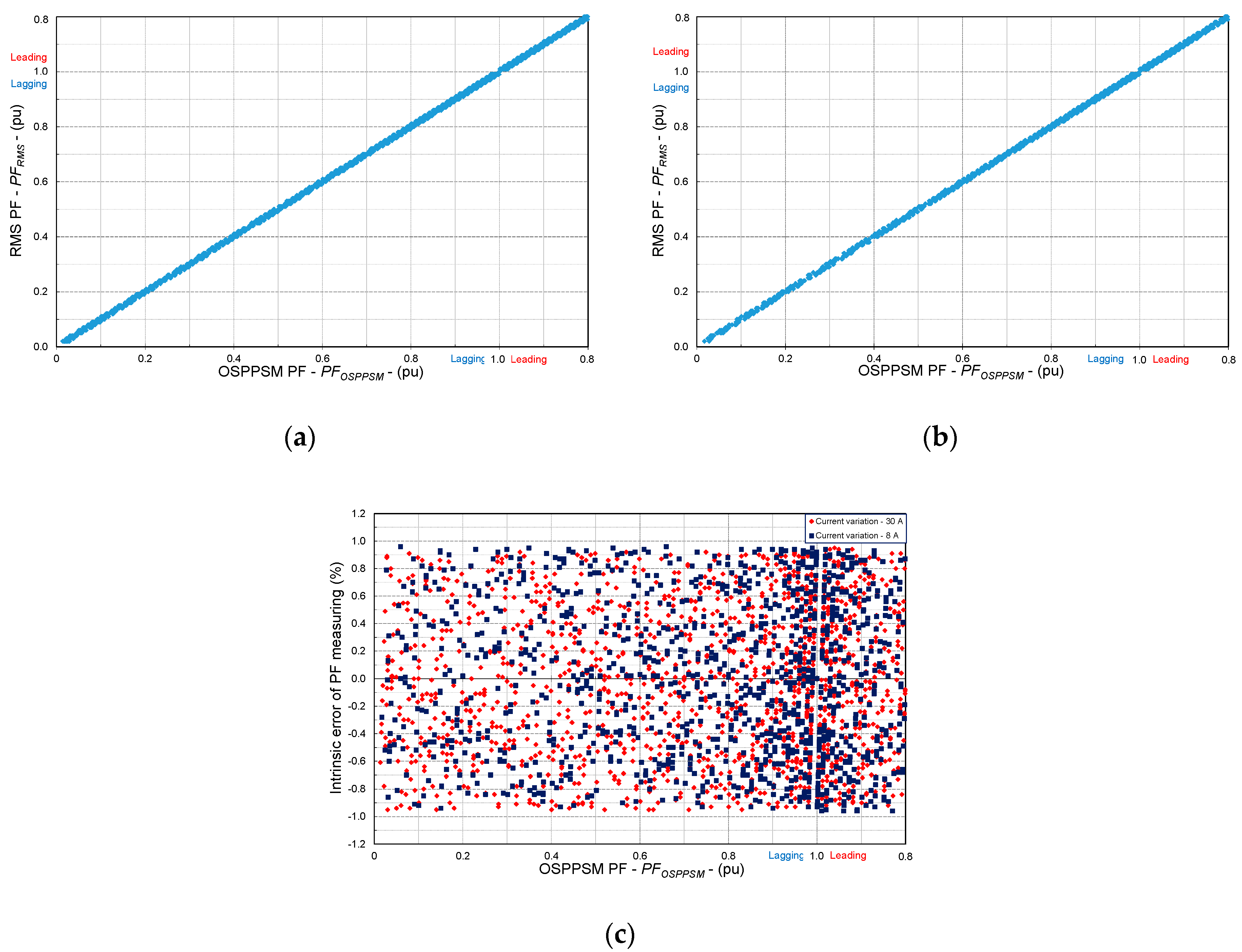
6.2.5. PF Variation Test

Table 11. PF variation test (wattmeter and varmeter, voltage variation): maximum intrinsic error (%), MAPE (%), MRE (%), and standard deviation (%).

Test	Maximum Intrinsic Error			MAPE			MRE			Standard Deviation
	v = 0 V i = 30 A	v = 230 V i = 30 A	v = 256 V i = 30 A	v = 0 V i = 30 A	v = 230 V i = 30 A	v = 256 V i = 30 A	v = 0 V i = 30 A	v = 230 V i = 30 A	v = 256 V i = 30 A	v = 0 V i = 30 A	v = 230 V i = 30 A	v = 256 V i = 30 A
Wattmeter, PF:1	0.940	0.950	0.910	0.458	0.492	0.518	−0.011	−0.025	−0.004	0.529	0.557	0.578
Varmeter, PF:1	0.920	0.940	0.900	0.465	0.483	0.467	0.022	−0.022	0.029	0.529	0.546	0.528
Wattmeter, PF:0.5 lagging)	0.940	0.930	0.970	0.473	0.488	0.526	−0.046	0.035	0.028	0.546	0.557	0.579
Varmeter, PF:0.5 lagging	0.960	0.980	0.940	0.488	0.499	0.506	0.119	0.008	0.058	0.547	0.581	0.557
Wattmeter, PF:0.5 leading)	0.970	0.990	0.930	0.485	0.497	0.461	0.051	0.011	0.037	0.555	0.575	0.538
Varmeter, PF:0.5 leading	0.950	0.950	0.940	0.421	0.493	0.474	−0.044	0.009	0.009	0.494	0.557	0.544

shows the first assessment of the PF variation test. This test changed the voltage when the OSPPSM acted as a wattmeter and varmeter. Since the intrinsic error attained a 0.97% maximum value, the OSPPSM remained in accuracy class 1.

Table 12. PF variation test (wattmeter and varmeter, current variation): maximum intrinsic error (%), MAPE (%), MRE (%), and standard deviation (%).

Test	Maximum Intrinsic Error			MAPE			MRE			Standard Deviation
	v = 230 V i = 0 A	v = 230 V i = 30 A	v = 230 V i = 36 A	v = 230 V i = 0 A	v = 230 V i = 30 A	v = 230 V i = 36 A	v = 230 V i = 0 A	v = 230 V i = 30 A	v = 230 V i = 36 A	v = 230 V i = 0 A	v = 230 V i = 30 A	v = 230 V i = 36 A
Wattmeter, PF:1	0.910	0.980	0.940	0.472	0.483	0.454	0.100	−0.050	−0.048	0.507	0.552	0.520
Varmeter, PF:1	0.910	0.960	0.900	0.523	0.419	0.467	−0.020	0.028	0.064	0.581	0.502	0.531
Wattmeter, PF:0.5 lagging)	0.950	0.950	0.930	0.413	0.490	0.480	0.032	0.031	−0.035	0.493	0.555	0.542
Varmeter, PF:0.5 lagging	0.950	0.950	0.970	0.544	0.463	0.480	0.004	0.057	0.125	0.597	0.538	0.538
Wattmeter, PF:0.5 leading)	0.950	0.910	0.950	0.460	0.494	0.501	−0.014	−0.027	−0.028	0.541	0.556	0.567
Varmeter, PF:0.5 leading	0.930	0.950	0.950	0.450	0.466	0.492	0.026	−0.005	0.016	0.518	0.546	0.564

shows the second assessment of the PF variation test. This test changed the current when the OSPPSM acted as a wattmeter and varmeter. Since the intrinsic error reached a 0.98% maximum value, the OSPPSM remained in accuracy class 1.

6.2.6. Continuous Overload Test

Table 13. Continuous overload test: maximum intrinsic error (%), MAPE (%), MRE (%), and standard deviation (%).

Test	Maximum Intrinsic Error	MAPE	MRE	Standard Deviation
Voltmeter	0.9800	0.4734	0.0352	0.5483
Ammeter	0.9900	0.4789	−0.0099	0.5582
PF meter	0.8600	0.0041	0.0003	0.0484
Wattmeter	0.9900	0.5047	−0.0066	0.5813
Varmeter	0.9800	0.4991	−0.0113	0.5725

gives the results of the continuous overload test. The maximum intrinsic error was lower than 0.99%. Consequently, the OSPPSM continued in accuracy class 1.

6.3. Uncertainty Evaluation

Table 14. Fundamental variables: input quantities from 10 sets of simultaneous observation.

Measure k/Input Quantities	v (V)	i (A)	PF (p.u.)
1	236.86	1.02	0.670
2	237.10	1.01	0.670
3	236.48	1.04	0.680
4	236.64	1.03	0.670
5	236.86	1.03	0.670
6	236.25	1.05	0.670
7	237.34	0.99	0.670
8	237.38	1.00	0.670
9	236.95	1.03	0.670
10	236.73	1.05	0.670

shows 10 independent sets of simultaneous observations for the three fundamental variables v, i, and PF (cos φ). Because the variables were simultaneously measured, they were correlated. Evidently, these correlations should be taken into account in the uncertainty evaluation of derived variables p and q.

Table 15. Fundamental variables and standard uncertainty.

Fundamental Variables	Mean	Standard Uncertainty	Standard Uncertainty (%)	Correlation Coefficients
v (V)	236.859	0.1130	0.00047	$\rho ({\mu }_v,{\mu }_i)$= −0.900
i (A)	1.0248	0.0064	0.0062	$\rho ({\mu }_i,{\mu }_{PF})$= 0.262
PF(p.u.)	0.6710	0.0010	0.0015	$\rho ({\mu }_v,{\mu }_{PF})$= −0.373

summarizes the standard uncertainty results for the fundamental variables. Accordingly,

Table 16. Fundamental variables and absolute accuracy.

Fundamental Variables	Absolute Accuracy
v (V)	$A{A}_v=\mathrm{InputReadingVoltage}\pm 0.1130$
i (A)	$A{A}_i=\mathrm{InputReadingCurrent}\pm 0.0064$
PF (p.u.)	$A{A}_{PF}=\mathrm{InputReadingPF}\pm 0.001$

shows the absolute precision of these variables in relation to the recommendations and requirements of the JCGM guide 100:2008 [84].

The relationship between the derived and the fundamental variables is described in Section 3. After the application of Equations (13) and (14),

Table 17. Derived variables and calculated values for derived quantities p and q.

Relationship between Variables	Estimate Value of Derived Variables	Combined Uncertainty	Combined Uncertainty (%)
$p=v·i·\cos \phi$ (W)	162.880	1.031	0.0063
$q=v·i·\sin \phi$ (VAr)	179.977	1.010	0.0056
Correlation coefficient	$\rho ({\mu }_p,{\mu }_q)$= 0.901

gives the standards uncertainties for the derived variables, according to Reference [28].

The results in

Table 18. Derived variables and absolute accuracy.

Derived Variables	Absolute Accuracy
p (W)	$A{A}_p=\mathrm{CalculatedActivePower}\pm 1.031$
q (VAr)	$A{A}_q=\mathrm{CalculatedReactivePower}\pm 1.010$

reflect the absolute accuracy of the derived variables, according to the JCGM guide 100:2008 [84].

As can be observed in the results of the uncertainty evaluation, the maximum uncertainty percentage was achieved for variable p, with a 0.0063% value, whereas the rest of the variables had lower values. In order to achieve a 99% confidence level (${\alpha }^{set}$ = 1%) when evaluating uncertainty, the minimum number of samples required for the active power measurement, according to Equation (17), is:

$$n_{s\text{-}\min }\ge {\left(\frac{2.58\times 1.031}{1}\right)}^2=7.08$$

(18)

and for the reactive power measurement:

$$n_{s\text{-}\min }\ge {\left(\frac{2.58\times 1.011}{1}\right)}^2=6.81$$

(19)

The 10 samples taken were sufficient to fulfill the set confidence level of 99%.

7. Conclusions and Discussion

This research study developed and successfully calibrated a new prototype of an accurate low-cost OSPPSM for collecting generation/load profiles at temporal high-resolution in real-world PV household-prosumer facilities. This OSPPSM was based on the Arduino open-source electronic platform. Input data were gathered with a set of sensors based on Arduino components. The NILM approach used in the OSPPSM makes it ideal for measuring electrical variables without modifying the monitored household.

This prototype has a number of advantages. More specifically, it determines fundamental and derived electrical variables in conformity with the IEC 61000-4-30 standard. The stationary analysis has a 10-cycle analysis window with a sampling rate of 1 kHz. Thanks to its dual board, the computational time is extremely fast. In fact, the OSPPSM is able to perform real-time monitoring with temporal high-resolution data, every 0.25 s (4 Hz). Evidently, this real-time calculation capacity and the big-data support in the cloud have promising applications, especially all that concerns the provision of advanced energy services for PV household-prosumers. The design of these services is based on the training and validation of models. However, this requires temporal high-resolution data for generation/load profiles that can be collected by using this prototype in real-world household facilities. It should be highlighted that these services account for the effects of both the fast short-term fluctuations of input profiles (<4 Hz) and their hourly/daily/weekly/monthly variability.

Another promising application of the prototype is the verification of household status by using a computer or mobile device that is able to perform the appropriate actions.

This prototype was calibrated as accuracy class 1, according to IEC standards for power smart meters. This was confirmed by the results of the calibration standard tests, in which there was a maximum error of 0.99% and a maximum uncertainty of 0.0063%. Moreover, the Kolmogorov-Smirnov tests performed on the OSPPSM, working as an ammeter and PF meter, showed uniform distributions of the intrinsic error distributions. This highlights the accuracy of the OSPPSM.

Furthermore, the prototype design features easy-to-obtain hardware and open-source software. This means that it is freely accessible to researchers and users in general for their own design and use in a non-intrusive way. With no loss of accuracy and uncertainty, the cost of this prototype is considerably lower than commercially available power-energy loggers (about 1400 €). It also has equivalent measurement functionalities without cloud data uploading.

The results obtained in this research justify the continuation and further development of the OSPPSM prototype. Further research will focus on building additional OSPPSMs and testing them in real-world scenarios by deploying a network of OSPPSMs in different PV household-prosumers. For the benefit of the research community, an open web interface will be designed to visualize the main electrical variables at temporal high-resolution of the monitored PV household-prosumers.

References

1. Elma, O.; Tascıkaraglu, A.; Ince, A.T.; Selamogulları, U.S. Implementation of a dynamic energy management system using real time pricing and local renewable energy generation forecasts. Energy 2017, 134, 206–220. [Google Scholar] [CrossRef]
2. Hosseinnia, H.; Tousi, B. Optimal operation of DG-based micro grid (MG) by considering demand response program (DRP). Electr. Pow. Syst. Res. 2019, 167, 252–260. [Google Scholar] [CrossRef]
3. Oprea, S.V.; Bara, A.; Ileana Uță, A.; Pirjan, A.; Căruțașu, G. Analyses of distributed generation and storage effect on the electricity consumption curve in the smart grid context. Sustainability 2018, 10, 2264. [Google Scholar] [CrossRef]
4. Morales-Velazquez, L.; Romero-Troncoso, R.J.; Herrera-Ruiz, G.; Morinigo-Sotelo, D.; Osornio-Rios, R.A. Smart sensor network for power quality monitoring in electrical installations. Measurement 2017, 103, 133–142. [Google Scholar] [CrossRef]
5. Angrisani, L.; Bonavolonta, F.; Liccardo, A.; Schiano Lo Moriello, R.; Serino, F. Smart power meters in augmented reality environment for electricity consumption awareness. Energies 2018, 11, 2303. [Google Scholar] [CrossRef]
6. Viciana, E.; Alcayde, A.; Montoya, F.; Baños, R.; Arrabal-Campos, F.; Zapata-Sierra, A.; Manzano-Agugliaro, F. OpenZmeter: An efficient low-cost energy smart meter and power quality analyser. Sustainability 2018, 10, 4038. [Google Scholar] [CrossRef]
7. Robles Algarín, C.; Sevilla Hernández, D.; Restrepo Leal, D. A low-cost maximum power point tracking system based on neural network inverse model controller. Electronics 2018, 7, 4. [Google Scholar] [CrossRef]
8. Abate, F.; Carratu, M.; Liguori, C.; Paciello, V. A low cost smart power meter for IoT. Measurement 2019, 136, 59–66. [Google Scholar] [CrossRef]
9. Schlund, J.; German, R. A control algorithm for a heterogeneous virtual battery storage providing FCR power. In Proceedings of the IEEE International Conference on Smart Grid and Smart Cities, Singapore, Singapore, 23–26 July 2017; pp. 61–66. [Google Scholar] [CrossRef]
10. Megel, O.; Mathieu, J.; Andersson, G. Scheduling distributed energy storage units to provide multiple services. In Proceedings of the IEEE Power Systems Computation Conference, Wroclaw, Poland, 18–22 August 2014; pp. 1–7. [Google Scholar] [CrossRef]
11. Steber, D.; Bazan, P.; German, R. SWARM—Strategies for providing frequency containment reserve power with a distributed battery storage system. In Proceedings of the IEEE International Energy Conference, Leuven, Belgium, 4–8 April 2016; pp. 1–7. [Google Scholar] [CrossRef]
12. Hernandez, J.C.; Sanchez-Sutil, F.; Vidal, P.G.; Rus-Casas, C. Primary frequency control and dynamic grid support for vehicle-to-grid in transmission systems. Int. J. Electr. Power Energy Syst. 2018, 100, 152–166. [Google Scholar] [CrossRef]
13. Litjens, G.B.M.A.; Worrell, E.; Van Sark, W.G.J.H.M. Economic benefits of combining selfconsumption enhancement with frequency restoration reserves provision by photovoltaic-battery systems. Appl. Energy 2018, 223, 172–187. [Google Scholar] [CrossRef]
14. Braun, M.; Büdenbender, K.; Magnor, D.; Jossen, A. Photovoltaic self-consumption in Germany: Using lithium-ion storage to increase self-consumed photovoltaic energy. In Proceedings of the 24th European Photovoltaic Solar Energy Conference, Hamburg, Germany, 21–25 September 2009; pp. 1–7. [Google Scholar]
15. Bruch, M.; Müller, M. Calculation of the cost-effectiveness of a PV battery system. Energy Procedia 2014, 46, 262–270. [Google Scholar] [CrossRef]
16. Schreiber, M.; Hochloff, P. Capacity-dependent tariffs and residential energy management for PV storage systems. In Proceedings of the IEEE Power and Energy Society General Meeting, Vancouver, BC, Canada, 21–25 July 2013; pp. 1–5. [Google Scholar] [CrossRef]
17. Linssen, J.; Stenzel, P.; Fleer, J. Techno-economic analysis of photovoltaic battery systems and the influence of different consumer load profiles. Appl. Energy 2017, 185, 2019–2025. [Google Scholar] [CrossRef]
18. Luthander, R.; Widen, J.; Nilsson, D.; Palm, J. Photovoltaic self-consumption in buildings: A review. Appl. Energy 2015, 142, 80–94. [Google Scholar] [CrossRef] [Green Version]
19. Fridgen, G.; Kahlen, M.; Ketter, W.; Riegera, A.; Thimmel, M. One rate does not fit all: An empirical analysis of electricity tariffs for residential microgrids. Appl. Energy 2018, 210, 800–814. [Google Scholar] [CrossRef] [Green Version]
20. Murray, D.; Stankovic, L.; Stankovic, V. An electrical load measurements dataset of United Kingdom households from a two-year longitudinal study. Sci. Data 2017, 4, 1–12. [Google Scholar] [CrossRef] [PubMed]
21. Kolter, J.Z.; Johnson, M.J. REDD: A public data set for energy disaggregation research. In Proceedings of the KDD Workshop on Data Mining Applications in Sustainability, San Diego, CA, USA, 21 August 2011; pp. 1–6. [Google Scholar]
22. Anderson, K.; Ocneanu, A.F.; Benitez, D.; Carlson, D.; Rowe, A.; Berges, M. BLUED: A Fully labeled public dataset for event-based non-intrusive load monitoring research. In Proceedings of the 2nd KDD Workshop on Data Mining Applications in Sustainability, Beijing, China, 12–16 August 2012; pp. 1–5. [Google Scholar]
23. Energy Saving Trust, Department of Energy and Climate Change (DECC); Final Report; Department for Environment, Food & Rural Affairs (DEFRA) Household Electricity Survey: London, UK, 2012.
24. Makonin, S.; Popowich, F.; Bartram, L.; Gill, B.; Bajic, I.V. A public dataset for load disaggregation and eco-feedback research. In Proceedings of the IEEE Electrical Power and Energy Conference, Halifax, NS, Canada, 21–23 August 2013; pp. 1–6. [Google Scholar] [CrossRef]
25. Makonin, S.; Ellert, B.; Bajic, I.V.; Popowich, F. Electricity, water, and natural gas consumption of a residential house in Canada from 2012 to 2014. Sci. Data 2016, 3, 160037. [Google Scholar] [CrossRef] [PubMed] [Green Version]
26. Hebrail, G.E.R.; Barard, A.E.R. Individual Household Electric Power Consumption Data Set (IhepcDS). Available online: https://archive.ics.uci.edu/ml/datasets/Individual+household+electric+power+ consumption (accessed on 22 June 2019).
27. Kelly, J.; Knottenbelt, W. The UK-DALE dataset, domestic appliance-level electricity demand and whole-house demand from five UK homes. Sci. Data 2015, 2, 150007. [Google Scholar] [CrossRef] [PubMed] [Green Version]
28. Ridi, A.; Gisler, C.; Hennebert, J. ACS-F2—A new database of appliance consumption signatures. In Proceedings of the 6th International Conference on Soft Computing and Pattern Recognition, Tunis, Tunisia, 11–14 August 2014; pp. 145–150. [Google Scholar] [CrossRef]
29. Reinhardt, A.; Baumann, P.; Burgstahler, D.; Hollick, M.; Chonov, H.; Werner, M.; Steinmetz, R. On the accuracy of appliance identification based on distributed load metering data. In Proceedings of the Sustainable Internet and ICT for Sustainability, Pisa, Italy, 4–5 October 2012; pp. 1–6. [Google Scholar]
30. Beckel, C.; Kleiminger, W.; Cicchetti, R.; Staake, T.; Santini, S. The ECO data set and the performance of non-intrusive load monitoring algorithms. In Proceedings of the 1st ACM Conference on Embedded Systems for Energy-Efficient Buildings, Memphis, TN, USA, 3–6 November 2014; pp. 80–89. [Google Scholar] [CrossRef]
31. Barker, S.; Mishra, A.; Irwin, D.; Cecchet, E.; Shenoy, P. Smart: An open data set and tools for enabling research in sustainable homes. In Proceedings of the 2nd KDD Workshop on Data Mining Applications in Sustainability, Beijing, China, 12–16 August 2012; pp. 1–6. [Google Scholar]
32. Bendato, I.; Bonfiglio, A.; Brignone, M.; Delfino, F.; Pampararo, F.; Procopio, R.; Rossi, M. Design criteria for the optimal sizing of integrated photovoltaic-storage systems. Energy 2018, 149, 505–515. [Google Scholar] [CrossRef]
33. Wolisz, H.; Schütz, T.; Blanke, T.; Hagenkamp, M.; Kohrn, M.; Wesseling, M.; Müller, D. Cost optimal sizing of smart buildings’ energy system components considering changing end-consumer electricity markets. Energy 2017, 137, 715–728. [Google Scholar] [CrossRef]
34. Dargahi, A.; Ploix, S.; Soroudi, A.; Wurtz, F. Optimal household energy management using V2H flexibilities. COMPEL Int. J. Comp. Math. Electr. Electron. Eng. 2014, 33, 777–793. [Google Scholar] [CrossRef]
35. Lim, Y.S.; Tang, J.H. Experimental study on flicker emissions by photovoltaic systems on highly cloudy region: A case study in Malaysia. Renew. Energy 2014, 64, 61–70. [Google Scholar] [CrossRef]
36. Saleh, M.; Meek, L.; Masoum, M.A.; Abshar, M. Battery-less short-term smoothing of photovoltaic generation using sky camera. IEEE Trans. Ind. Inform. 2018, 14, 403–414. [Google Scholar] [CrossRef]
37. Marcos, J.; Marroyo, L.; Lorenzo, E.; Alvira, D.; Izco, E. Power output fluctuations in large scale PV plants: One year observations with one second resolution and a derived analytic model. Prog. Photovolt. Res. Appl. 2011, 19, 218–227. [Google Scholar] [CrossRef]
38. Widen, J.; Wackelgard, E.; Lund, P.D. Options for improving the load matching capability of distributed photovoltaics: Methodology and application to high latitude data. Sol. Energy 2009, 83, 1953–1966. [Google Scholar] [CrossRef]
39. Dougal, R.A.; Liu, S.; White, R.E. Power and life extension of battery–ultracapacitor hybrids. IEEE Trans. Compon. Packag. Technol. 2002, 25, 120–131. [Google Scholar] [CrossRef]
40. Wright, A.; Firth, S. The nature of domestic electricity-loads and effects of time averaging on statistics and on-site generation calculations. Appl. Energy 2007, 84, 389–403. [Google Scholar] [CrossRef] [Green Version]
41. Omar, N.; Monem, M.A.; Firouz, Y.; Salminen, J.; Smekens, J.; Hegazy, O.; Gaulous, H.; Mulder, G.; Van den Bossche, P.; Coosemans, T.; et al. Lithium iron phosphate based battery. Assessment of the aging parameters and development of cycle life model. Appl. Energy 2014, 113, 1575–1585. [Google Scholar] [CrossRef]
42. Ruddell, A.J.; Dutton, A.G.; Wenzl, H.; Ropeter, C.; Sauer, D.U.; Merten, J.; Orfanogiannis, C.; Twidell, J.W.; Vezin, P. Analysis of battery current microcycles in autonomous renewable energy systems. J. Power Sources 2002, 112, 531–546. [Google Scholar] [CrossRef]
43. Jabbar Mnati, M.; Van den Bossche, A.; Farhood Chisab, R. A smart voltage and current monitoring system for three phase inverters using an android smartphone application. Sensors 2017, 17, 872. [Google Scholar] [CrossRef]
44. Robles Algarín, C.; Callejas Cabarcas, J.; Polo Llanos, A. Low-cost fuzzy logic control for greenhouse environments with web monitoring. Electronics 2017, 6, 71. [Google Scholar] [CrossRef]
45. Fuentes, M.; Vivar, M.; Burgos, J.M.; Aguilera, J.; Vacas, J.A. Design of an accurate, low-cost autonomous data logger for PV system monitoring using ArduinoTM that complies with IEC standards. Sol. Energy Mater. Sol. Cells 2014, 130, 529–543. [Google Scholar] [CrossRef]
46. Amiry, H.; Benhmida, M.; Bendaoud, R.; Hajjaj, C.; Bounouar, S.; Yadir, S.; Raïs, K.; Sidki, M. Design and implementation of a photovoltaic I-V curve tracer: Solar modules characterization under real operating conditions. Energy Convers. Manag. 2018, 69, 206–216. [Google Scholar] [CrossRef]
47. Cano Ortega, A.; Sanchez Sutil, F.J.; Hernandez, J.C. Power factor compensation using teaching learning based optimization and monitoring system by cloud data logger. Sensors 2019, 19, 2172. [Google Scholar] [CrossRef] [PubMed]
48. Visalatchi, S.; Sandeep, K.K. Smart energy metering and power theft control using arduino & GSM. In Proceedings of the 2nd International Conference for Convergence in Technology, Mumbai, India, 7–9 April 2017; pp. 1–6. [Google Scholar] [CrossRef]
49. Arif, A.; Al-Hussain, M.; Al-Mutairi, N.; Al-Ammar, E.; Khan, Y.; Malik, N. Experimental study and design of smart energy meter for the smart grid. In Proceedings of the International Renewable and Sustainable Energy Conference, Ouarzazate, Morocco, 7–9 March 2013; pp. 1–6. [Google Scholar] [CrossRef]
50. Abubakar, I.; Khalid, S.N.; Mustafa, M.W.; Shareef, H.; Mustapha, M. Calibration of ZMPT101b voltage sensor module using polynomial regression for accurate load monitoring. ARPN J. Eng. Appl. Sci. 2013, 12, 1076–1084. [Google Scholar]
51. Jimenez-Castillo, G.; Muñoz-Rodriguez, F.J.; Rus-Casas, C.; Hernandez, J.C.; Tina, G.M. Monitoring PWM signals in stand-alone photovoltaic systems. Measurement 2019, 134, 412–425. [Google Scholar] [CrossRef]
52. Tarasiuk, T.; Szweda, M.; Tarasiuk, M. Estimator–analyzer of power quality: Part II—Hardware and research results. Measurement 2011, 44, 248–258. [Google Scholar] [CrossRef]
53. Arduino Nano. Available online: https://store.arduino.cc/arduino-nano (accessed on 22 June 2019).
54. Arduino Mega. Available online: https://store.arduino.cc/mega-2560-r3 (accessed on 15 June 2019).
55. Adafruit Industries Ltd. Available online: https://www.adafruit.com/product/904 (accessed on 22 June 2019).
56. IEC. IEC Standard 61000-4-7. Electromagnetic Compatibility (EMC): Testing and Measurement Techniques—General Guide on Harmonics and Interharmonics Measurements and Instrumentation, for Power Supply Systems and Equipment Connected Thereto; International Electrotechnical Commission: Geneva, Swizerland, 2008. [Google Scholar]
57. Ramos, P.M.; Janeiro, F.M.; Girao, P.S. Uncertainty evaluation of multivariate quantities: A case study on electrical impedance. Measurement 2016, 78, 397–411. [Google Scholar] [CrossRef]
58. Apetrei, D.; Silvas, I.; Albu, M.; Postolache, P.; Neurohr, R. Voltage estimation in power distribution networks. a case study on data aggregation and measurement uncertainty. In Proceedings of the International Workshop on Advanced Methods for Uncertainty Estimation in Measurement, Bucharest, Romania, 6–7 July 2009; pp. 1–6. [Google Scholar] [CrossRef]
59. IEC. IEC Standard 61000-4-30. Electromagnetic Compatibility (EMC): Testing and Measurement Techniques—Power Quality Measurement Methods; International Electrotechnical Commission: Geneva, Swizerland, 2015. [Google Scholar]
60. Webster, J.G. Electrical, Measurement, Signal Processing, and Displays; CRC Press LLC: Boca Raton, FL, USA, 2004. [Google Scholar]
61. Arduino Uno Rev3. Available online: https://store.arduino.cc/arduino-uno-rev3 (accessed on 22 June 2019).
62. WEMOS Electronics. Available online: https://wiki.wemos.cc/products:d1:d1 (accessed on 22 June 2019).
63. Dechang Electronics Co. Ltd. Available online: http://en.yhdc.com (accessed on 22 June 2019).
64. Firebase. Available online: https://firebase.google.com (accessed on 22 June 2019).
65. Arduino MKR WiFi 1010. Available online: https://store.arduino.cc/mkr-wifi-1010 (accessed on 22 June 2019).
66. Node MCU Arduino. Available online: https://www.nodemcu.com (accessed on 22 June 2019).
67. Interplus Industry Co. Ltd. Available online: http://www.interplus-industry.fr/index.php? option=com_content&view=article&id=52&Itemid=173&lang=en (accessed on 22 June 2019).
68. STC013 Dechang Electronics Co. Ltd. Available online: http://en.yhdc.com/product/ SCT013-401.html. (accessed on 22 June 2019).
69. Texas Instruments. Available online: http://www.ti.com/lit/ds/symlink/ads1114.pdf (accessed on 22 June 2019).
70. Arduino Software. Available online: https://www.arduino.cc/en/Main/Software (accessed on 22 June 2019).
71. Sánchez, H.; Gonzalez-Contreras, C.; Agudo, J.E.; Macías, M. IoT and ITV for interconnection, monitoring, and automation of common areas of residents. Appl. Sci. 2017, 7, 696. [Google Scholar] [CrossRef]
72. Sridharana, M.; Devi, R.; Dharshini, C.S.; Bhavadarani, M. IoT based performance monitoring and control in counter flow double pipe heat exchanger. Internet Things 2019, 5, 34–40. [Google Scholar] [CrossRef]
73. Ramírez-Gil, J.G.; Giraldo Martínez, G.O.; Morales Osorio, J.G. Design of electronic devices for monitoring climatic variables and development of an early warning system for the avocado wilt complex disease. Comput. Electron. Agric. 2018, 153, 134–143. [Google Scholar] [CrossRef]
74. Radmannia, S.; Naderzad, M. IoT-based electrosynthesis ecosystem. Internet Things 2018, 3, 46–51. [Google Scholar] [CrossRef]
75. Da Cruz, M.A.; Rodrigues, J.J.; Lorenz, P.; Solic, P.; Al-Muhtadi, J.; Albuquerque, V.H.C. A proposal for bridging application layer protocols to HTTP on IoT solutions. Future Gener. Comput. Syst. 2019, 97, 145–152. [Google Scholar] [CrossRef]
76. Al-Ali, A.R.; Zualkernan, I.A.; Rashid, M.; Gupta, R.; AliKarar, M. Smart home energy management system using IoT and big data analytics approach. IEEE Trans. Consum. Electron. 2017, 63, 4. [Google Scholar] [CrossRef]
77. Moghimi, M.; Liu, J.; Jamborsalamati, P.; Rafi, F.; Rahman, S.; Hossain, J.; Stegen, S.; Lu, J. Internet of things platform for energy management in multi-microgrid system to improve neutral current compensation. Energies 2018, 11, 3102. [Google Scholar] [CrossRef]
78. IEC. IEC Standard 60051-1. Direct Acting Indicating Analogue Electrical Measuring Instruments and their Accessories: Definitions and General Requirements Common to All Parts; International Electrotechnical Commission: Geneva, Swizerland, 2016. [Google Scholar]
79. IEC. IEC Standard 60050-311. International Electrotechnical Vocabulary: Electrical and Electronic Measurements and Measuring Instruments: General Terms Relating to Measurements; International Electrotechnical Commission: Geneva, Swizerland, 2001. [Google Scholar]
80. IEC. IEC Standard 60051-2. Direct Acting Indicating Analogue Electrical Measuring Instruments and their Accessories: Special Requirements for Ammeters and Voltmeters; International Electrotechnical Commission: Geneva, Swizerland, 2018. [Google Scholar]
81. IEC. IEC Standard 60051-3. Direct Acting Indicating Analogue Electrical Measuring Instruments and their Accessories: Special Requirements for Wattmeters and Varmeters; International Electrotechnical Commission: Geneva, Swizerland, 2018. [Google Scholar]
82. IEC. IEC Standard 60051-5. Direct Acting Indicating Analogue Electrical Measuring Instruments and Their Accessories: Special Requirements for Phase Meters, Power Factor Meters and Synchroscopes; International Electrotechnical Commission: Geneva, Swizerland, 2017. [Google Scholar]
83. IEC. IEC Standard 60051-9. Direct acting indicating analogue electrical measuring instruments and their accessories: Recommended test methods; International Electrotechnical Commission: Geneva, Swizerland, 2019. [Google Scholar]
84. JCGM/WG 1. Evaluation of Measurement Data—Guide to the Expression of Uncertainty in Measurement, GUM 50; JCGM: Sèvres, France, 2008; 134p. [Google Scholar] [CrossRef]
85. Bell, S. Measurement Good Practice Guide No. 11 (Issue 2)—A Beginner’s Guide to Uncertainty of Measurement; National Physical Laboratory: Teddington, UK, 2001. [Google Scholar]
Figure 1. OSPPSM prototype.
Electronics 08 00878 g001
Figure 2. Hardware block diagram of the OSPPSM.
Electronics 08 00878 g002
Figure 3. Wiring diagram of the OSPPSM.
Electronics 08 00878 g003
Figure 4. Process timeline for the OSPPSM.
Electronics 08 00878 g004
Figure 5. Flowchart for the measurement and computation of the electric variable: AUR3 board.
Electronics 08 00878 g005
Figure 6. Flowchart for cloud data uploading: AD1R1 board.
Electronics 08 00878 g006
Figure 7. Test equipment and OSPPSM in the laboratory at Jaen university.
Electronics 08 00878 g007
Figure 8. Voltmeter test: (a) OSPPSM vs. RMS voltage. (b) Intrinsic error of voltage measuring.
Electronics 08 00878 g008
Figure 9. Ammeter test: (a) OSPPSM vs. RMS current. (b) Intrinsic error of current measuring.
Electronics 08 00878 g009
Figure 10. PF meter test: (a) 30 A, OSPPSM vs. RMS PF. (b) 8 A, OSPPSM vs. RMS PF. (c) Intrinsic error of PF measuring, 8 A and 30 A.
Electronics 08 00878 g010
Figure 11. Wattmeter test: (a) OSPPSM vs. RMS active power. (b) Intrinsic error of active power measuring.
Electronics 08 00878 g011
Figure 12. Varmeter test: (a) OSPPSM vs. RMS reactive power. (b) Intrinsic error of reactive power measuring.
Electronics 08 00878 g012
Figure 13. Voltmeter test: (a) OSPPSM vs. RMS voltage. (b) Intrinsic error of voltage measuring.
Electronics 08 00878 g013
Figure 14. PF meter, wattmeter, and varmeter test: intrinsic error of different variables measuring the voltage variation.
Electronics 08 00878 g014
Figure 15. Ammeter test: (a) OSPPSM vs. RMS current. (b) Intrinsic error of current measuring.
Electronics 08 00878 g015
Figure 16. PF meter, wattmeter, and varmeter test: intrinsic error of different variable measuring for current variation.
Electronics 08 00878 g016
Figure 17. Voltmeter test: (a) OSPPSM vs. RMS voltage. (b) Intrinsic error of voltage measuring.
Electronics 08 00878 g017
Figure 18. Ammeter test: (a) OSPPSM vs. RMS current. (b) Intrinsic error of current measuring.
Electronics 08 00878 g018
Figure 19. PF meter test: Intrinsic error of PF measuring (PF: 0.5 lagging, 1, 0.5 leading).
Electronics 08 00878 g019
Figure 20. Wattmeter and varmeter test: Intrinsic error of different variable measuring.
Electronics 08 00878 g020