Abstract
In this paper we show how to efficiently implement parallel discrete simulations on multicore and GPU architectures through a real example of an application: a cellular automata model of laser dynamics. We describe the techniques employed to build and optimize the implementations using OpenMP and CUDA frameworks. We have evaluated the performance on two different hardware platforms that represent different target market segments: high-end platforms for scientific computing, using an Intel Xeon Platinum 8259CL server with 48 cores, and also an NVIDIA Tesla V100 GPU, both running on Amazon Web Server (AWS) Cloud; and on a consumer-oriented platform, using an Intel Core i9 9900k CPU and an NVIDIA GeForce GTX 1050 TI GPU. Performance results were compared and analyzed in detail. We show that excellent performance and scalability can be obtained in both platforms, and we extract some important issues that imply a performance degradation for them. We also found that current multicore CPUs with large core numbers can bring a performance very near to that of GPUs, and even identical in some cases.
1. Introduction
Discrete simulation methods encompass a family of modeling techniques which employ entities that inhabit discrete states and evolve in discrete time steps. Examples include models such as cellular automata (CA) and related lattice automata, such as lattice gas automata (LGA) or the lattice Boltzmann method (LBM), and also discretizations of continuos models, such as many stencil-based partial differential equation (PDE) solvers and particle methods based on fixed neighbor lists. They are powerful tools that have been widely used to simulate complex systems of very different kinds (in which a global behavior results from the collective action of many simple components that interact locally) and to solve systems of differential equations.
To accurately simulate real systems, the quality of the computed results very often depends on the number of data points used for the computations and on the complexity of the model. As a result, realistic simulations frequently involve excessive runtime and memory requirements for a sequential computer. Therefore, efficient parallel implementations of this kind of discrete simulation are extremely important. But this type of discrete algorithm has a strong parallel nature, because each is composed of many individual components or cells that are simultaneously updated. They also have a local nature, since the evolution of cells is determined by strictly local rules; i.e., each cell only interacts with a low number of neighboring cells. Thanks to this, they are very suitable to be implemented efficiently on parallel computers [1,2].
In this paper, we study the efficient parallel implementation of a real application of this type, a CA model of laser dynamics, on multicore and GPU architectures, employing the most commonly used software frameworks for these platforms today: OpenMP and CUDA, respectively. In both cases, we describe code optimizations that can speed-up the computation and reduce memory usage. In both cases we evaluated the performance on two different hardware platforms that represent different target market segments: a high-end chip intended for scientific computing or for servers, and on a consumer-oriented one. In the case of the multicore architecture, the performance has been evaluated on a dual socket server with 2 high-end Intel Xeon Platinum 8259CL processors (completing 48 cores between them) running on Amazon Web Server (AWS) Cloud, and also on a PC market Intel Core i9 9900 k processor. For the GPU architecture, we present the performance evaluation results of a high-end GPGPU NVIDIA Tesla V100 GPU running on AWS Cloud and on a consumer-oriented NVIDIA GeForce GTX 1050 TI. In all cases, we report speedups compared to a sequential implementation. The aim of this work was to extract lessons that may be helpful for practitioners implementing discrete simulations of real systems in parallel.
The considered application uses cellular automata, a class of discrete, spatially-distributed dynamical systems with the following characteristics: a spatial and temporally discrete nature, local interaction, and synchronous parallel dynamical evolution [3,4]. They can be described as a set of identical finite state machines (cells) arranged along a regular spatial grid, whose states are simultaneously updated by a uniformly applied state-transition function that refers to the states of their neighbors [5]. In the last few decades, CA has been successfully applied to build simulations of complex systems in a wide range of fields, including physics (fluid dynamics, magnetization in solids, reaction-diffusion processes), bio-medicine (viral infections, epidemic spreading), engineering (communication networks, cryptography), environmental science (forest fires, population dynamics), economics (stock exchange markets), theoretical computer science, etc. [6,7,8]. It is currently being very used, in particular, for simulations in geography (especially in urban development planning [9], future development of cities [10], and land use [11]) pedestrian or vehicular traffic [12,13], and bio-medicine (applied to physiological modeling; for example, for cancer [14], or epidemic modeling [15]).
The application studied here is a cellular automata model of laser dynamics introduced by Guisado et al., capable of reproducing much of the phenomenology of laser systems [16,17,18,19]. It captures the essence of a laser as a complex system in which its macroscopic properties emerge spontaneously due to the self-organization of its basic components. This model is a useful alternative to the standard modeling approach of laser dynamics, based on differential equations, in situations where the considered approximations are not valid, such as lasers being ruled by stiff differential equations, lasers with difficult boundary conditions, and very small devices. The mesoscopic character of the model also allowed us to get results impossible to be obtained by the differential equations, such as studying the evolution of its spatio-temporal patterns.
In order to reduce the runtime of laser simulations with this model by taking advantage of its parallel nature, a parallel implementation of it for computer clusters (distributed-memory parallel computers), using the message-passing programming paradigm, was introduced in [20,21]. It showed a good performance on dedicated computer clusters [22] and also on heterogeneous non-dedicated clusters with a dynamic load balancing mechanism [23].
Due to the excellent ratio performance/price and performance/power of graphics processing units (GPUs), it is very interesting to implement the model on them. GPUs are massively parallel graphics processors originally designed for running interactive graphics applications, but that can also be used to accelerate arbitrary applications, which is known as GPGPU (general purpose computation on a GPU) [24]. They can run thousands of programming threads in parallel, providing speedups mainly from ×10 to ×200 compared to a CPU (depending on the application and on the optimizations of its implementation), at very affordable prices. Therefore, GPUs have widespread use today in high performance scientific computing. Their architecture is formed by a number of multiprocessors, each of them with a number of cores. All cores of a multiprocessor share one memory unit called shared memory, and all multiprocessors share a memory unit called global memory.
A first version of a parallel implementation of the model for GPUs was presented in [25]. Even when that first implementation did not explore all the possible optimizations to boost the performance on that platform, it showed that the model could be successfully implemented on GPU. A speedup of on a NVIDIA GeForce GTX 285 (a consumer-oriented GPU intended for low-end users and gamers) compared to an Intel Core i5 750 with 4 cores at GHz was obtained. The GPU implementation described in the present paper improves on the previous one; it has been carefully optimized to extract all possible performance features from the GPU, and its performance has been evaluated not only on a consumer-oriented GPU, but also on a Tesla scientific, high-end GPU.
Another interesting parallel platform to implement discrete simulations on today is the multicore processor. Since around 2005, all general-purpose CPUs have implemented more than one CPU (or “core”) on the processor chip. For a decade, the number of cores in standard Intel ×86 processors was modest (mainly from 2 to 8). But in the last few years, high-end CPUs emerged in the market which include up to several dozen cores (now up to 18 cores for Intel Core i9 and up to 56 cores for Intel Xeon Platinum). Therefore, multicore CPUs can start to be competitive with GPUs to implement parallel discrete simulations, especially taking into account that parallelization with OpenMP is much easier than for GPUs. Therefore, we also present the first parallel implementation of the CA laser dynamics model for multicore architectures, and we compare its performance on current high-end multicore CPUs to the performance obtained on GPUs.
The remainder of the paper is organized as follows: Section 2 reviews the related work in the field of discrete simulations via cellular automata and their parallel implementation on multicore and GPU Architectures. Section 3 describes the methodology employed in this work, trying to give useful indications to researchers interested in parallelizing efficiently their own codes. Section 4 presents the results and discusses their interpretation and significance. Finally, Section 5 summarizes the contents of this paper, and the conclusions, and indicates interesting future work.
2. Related Work
Most parallel implementations of CA models on multicore processors or GPUs were presented after 2007. In the case of multicore processors, they became generalised only from 2005 onwards, and started to be used for parallel simulations in the years following. Regarding GPUs, before 2007 there were few works devoted to the parallel implementation of cellular automata models on GPUs, because they had to adapt somehow their application to a shading language (a special purpose programming language for graphics applications), such as OpenGL. An example is the paper from Gobron et al. [26], which studied a CA model for a biological retina obtaining a ×20 speedup compared to the CPU implementation. After the introduction in 2007 of CUDA (compute unified device architecture), a general purpose programming language for GPUs of the NVIDIA manufacturer, there was soon a multi-platform one called OpenCL; the usage of GPUs in scientific computing exploded.
Let us review some relevant parallel implementations of CA models on multicore CPUs and GPUs introduced from 2007 on.
Rybacki et al. [27] presented a study of the performances of seven different very simple cellular automata standard models running on a single core processor, a multi core processor, and a GPU. They found that the performance results were strongly dependent on the model to be simulated.
Bajzát et al. [28] obtained an order of magnitude increase in the performance of the GPU implementation of a CA model for an ecological system, compared to a serial execution.
Balasalle et al. [29] studied how to improve the performance of the GPU implementation of one of the simplest two-dimensional CAs—the game of life—by optimizing the memory access patterns. They found that careful optimizations of the implementation could produce a 65% improvement in runtime from a baseline implementation. However, they did not study other more realistic CA models.
Special interest has been devoted to GPU implementations of Lattice Boltzmann methods, a particular class of CA. Some works have been able to obtain spectacular speedups for them. For instance, [30] reported speedups of up to ×234 with respect to single-core CPU execution without using SSE instructions or multithreading.
Gibson et al. [31] presents the first thorough study of the performance of cellular automata implementations on GPUs and multi-core CPUs with respect to different standard CA parameters—lattice and neighborhood sizes, number of states, complexity of the state transition rules, number of generations, etc. They have studied a “toy application”, the “game of life” cellular automaton in two dimensions and two multi-state generalizations of it. They employed the OpenCL framework for the parallel implementation on GPUs and OpenMP for multi-core CPUs. That study is very useful for researchers, helping them choose the right CA parameters, when it is possible, by taking into account their impact in performance. Additionally, it helps to explain much of the variation found in reported speedup factors from literature. Our present work is different and complementary to that study in the sense that the game of life is a toy model very useful to study the dependence of performance on general CA parameters, but it is also very interesting to study the parallelization and performance of a real application instead of a toy model such as the game of life, as we do in this work.
3. Materials and Methods
3.1. Cellular Automaton Model for Laser Dynamics Simulation
We present parallel implementations for multicore CPUs and for GPUs of the cellular automaton model of laser dynamics introduced by Guisado et al. [16,17,18].
A laser system is represented in this model by a two-dimensional CA which corresponds to a transverse section of the active medium in the laser cavity.
Formally, the CA model is made of:
- (a)
- A regular lattice in a two-dimensional space of cells. Each lattice position is labelled by the indices . In order to avoid boundary problems and to best simulate the properties of a macroscopic system, we use periodic boundary conditions.
- (b)
- The state variables associated with each node . In the case of a laser system, we need two variables: one for the lasing medium and the other for the number of laser photons . is a boolean variable: 1 represents the excited state of the electron in the lasing medium in cell and 0 is the ground state. For the photons, is an integer variable in the range , where M is an upper limit that represent, the number of laser photons in cell . The state variables and represent “bunches” of real photons and electrons, the values of which are obviously smaller than the real number of photons and electrons in the system and are connected to them by a normalization constant.
- (c)
- The neighborhood of a cell. In a cellular automata the state variables can change depending on the neighboring cells. In the laser model studied here [16], the Moore neighborhood is employed: the neighborhood of a cell consists of the cell itself and the eight cells around it at positions north, south, east, west, northeast, southeast, northwest, and southwest.
- (d)
- The evolution rules that specify the state variables at time as a function of their state at time t. From a microscopic point of view the physics of a laser can be described by five processes:
- (i)
- The pumping of the ground state of the laser medium to the excited state. In this way energy is supplied to the lasing medium. This process is considered to be probabilistic: If , then with a probability .
- (ii)
- The stimulated emission by which a new photon is created when an excited laser medium cell surrounded by one or more photons decays to the ground state: If and the sum of the values of the laser photons states in its neighboring cells is greater than 1, then and .
- (iii)
- The non-radiative decaying of the excited state. After a finite time , an excited laser medium cell will go to the ground state without the generation of any photon.
- (iv)
- The photon decay. After a given time , photons escape and their number is decreased by one unit .
- (v)
- Thermal noise. In a real laser system, there is a thermal noise of photons produced by spontaneous emissions, and they cause the initial start-up of the laser action. Therefore in our CA model, a small number of photons (less than ) are added at random positions at each time step.
3.2. Sequential Implementation of the Model
The algorithmic description of the model using pseudo code is shown in Algorithms 1–4. The main program is described in Algorithm 1. The structure of the algorithm is based on a time loop, inside of which there is a data loop to sweep all the CA cells. At each time step, first, the lattice cell states are updated by applying the transition rules, and then the total populations of laser photons and electrons in the upper state are calculated by summing up the values of the state variables and for all the lattice cells. Because we are emulating a time evolution, the order of the transition rules for each time step can be switched. Of course, different orders get to slightly different particle quantities, but on the whole, CA evolution is similar. Algorithm 2 defines the implementation of the noise photon creation rule. The photon and electron decay rules and the evolution of temporal variables are described in Algorithm 3. Finally, Algorithm 4 describes the implementation of the pumping and stimulated emission rules.
In order to simulate a parallel evolution of all the CA cells, we use two copies of the matrix, called c and . In each time step, the new states of are written in and the updated values of this matrix are only copied to c after finishing with all the CA cells. In the algorithmic description of the implementation of the model, we used two temporal variables, and as time counters, where k distinguishes between the different photons that can occupy the same cell. When a photon is created, . After that, 1 is subtracted to for every time step, and the photon will be destroyed when . When an electron is initially excited, . Finally, 1 is subtracted to for every time step and the electron will decay to the ground level again when .
| Algorithm 1 Pseudo code description of the main program for the CA laser model. |
|
| Algorithm 2 Pseudo code diagram for the implementation of the noise photons rule. |
|
| Algorithm 3 Pseudo code diagram for the implementation of the photon and electron decay and evolution of temporal variables’ rules. |
|
| Algorithm 4 Pseudo code diagram for the implementation of the pumping and stimulated emission rules. |
|
3.3. Parallel Frameworks for Efficient CA Laser Dynamics Simulation
Algorithms described in previous Section 3.2 arise from a conversion of the physical processes and differential equation systems that represent the CA laser model. The efficient execution of these algorithms in parallel platforms to generate fast simulations of a bunch of different input parameters requires many specific considerations for each hardware platforms. To begin with, modern, out-of-order execution superscalar processors achieve an almost optimal time execution of operations when operands reside in CPU registers. That is, they reach the so-called –– of the algorithm, those being the most patent bottlenecks of the real dependences among operations and the difficult branch predictions. In fact, taking some simple assumptions around these bottlenecks, some authors have proposed simple processor performance models that predict computing times with enough accuracy [32]. Above this, when many operations cannot be executed over CPU registers, memory model is the other crucial factor.
In relation with our CA model, a simple inspection of the code and of the data evolution brings to light that memory usage is massive and that an elevated branch misprediction ratio is expected. The first assertion is obvious: matrices that contain , , , and suppose many megabytes for those lattice widths that emulate a correct behavior of the laser dynamics. The second assertion comes mainly from two code features: the use of random values in many decisions representing the particle evolution, and the difficult-to-predict values that particle states take along the life of the simulation. While this paper concentrates in a laser dynamics model, it is obvious that these features may be present in many CA simulations, mostly when cooperative phenomena are expected. What is more relevant is the existence of many branches (some of them in the form of nested conditional structures) in the "hot spot" zones implies that GPU implementations would suffer from an important deceleration. This is due to the inherent so-called thread divergence [33] that GPU compilers introduce in these cases, which is one of the main reasons why performance on these platforms diminishes.
Taking into account previous considerations, an accurate timing characterization of main sequential algorithm pieces was done. This analysis concludes that:
- -
- More than 80% of the mean execution time is spent in stimulated emission and pumping rules. What is more, their execution times have a considerable variance: minimum times are around five times lower than maximum times. This asserts the effect of random values and the difficult to predict evolution of different cell particles.
- -
- Random number computation supposes around the 70% of the pumping rule time.
- -
- The rest of time resides mainly in photon and electron decay. The oscillatory behavior of particle evolution during the stationary phase implies also a considerable variance in these times. This is even more exaggerated during transient evolution.
- -
- Noise photon rule timing is negligible, because this rule has a much smaller number of iterations than the other rules.
Previous facts make necessary the introduction of at least the next changes in both OpenMP and GPU code implementations (see https://github.com/dcagigas/Laser-Cellular-Automata):
- -
- Of course, avoiding non re-entrant functions, such as simple random numbers generators. Even more, although generating a seed for each thread should be enough to make random generation independent among threads, the deep inner real data dependencies that random functions contain last in the mean longer than the rest of an iteration step. An implementation similar to that of the library is preferable; that is, a seed for each cell , which preserves a good random distribution while it accelerates each step around 40%.
- -
- As only one electron per cell is allowed, suppressing the matrix. Thus, it is considered that if is zero, the electron is not excited; and it is excited elsewhere.
- -
- Eliminating the refresh of c matrix (which supposes copying long matrices) with values of (line 9 of Algorithm 1), by using pointers to these two matrices and swapping these pointers at the end of each iteration step.
In order to generate the random numbers, we have used the permuted congruential generator (PCG) [34], a pseudorandom number generator based on a combination of permutation functions on tuples and a base linear congruential generator. This generator was selected because it has several desirable properties: it has proven to be statistically good, very fast, and its internal state does not need a very large memory space. It is also suitable to be implemented in parallel both for multicore and for GPU architectures.
The source code of the different implementations and the results achieved are available at https://github.com/dcagigas/Laser-Cellular-Automata. The source code is under GPL v3 license. Researchers can download and modify the code freely to run their own particular laser dynamic simulations.
3.3.1. OpenMP Framework
Previous improvements are quite easy to detect and to implement. However, there are further enhancements that speedup a CA simulation even more when running an OpenMP implementation over multicore platforms. As a result, apart from the OPENMP_NOT_OPTIMIZED version, an optimized one (called simply OPENMP) can be downloaded from the previous page. For the sake of clarity, these further enhancements are grouped and listed in the following points. Moreover, they have been marked in the source code with the symbol @.
- -
- After a deeper examination of laser dynamics evolution, it was detected that very few cells contained more than one photon during the stationary evolution. Thus, the habitual matrix arrangement of variable ; that is, when consecutively storing the M values for each cell, is switched by the following one. All the cells are stored consecutively for each of the M possible photons. In terms of the C++ code, this three-dimensional matrix is represented by: (see matrix in the code). The new arrangement implies that all elements of are continuously used and then cached, but the rest of elements are scarcely used, so they do not consume precious cache lines. On the contrary, if the habitual matrix arrangement had been used, it would have wasted many cache bytes (almost only 1 of each M element would have been really used during the stationary period). The rest of code pieces where this matrix is manipulated are not decelerated by the new arrangement; e.g., very few cells generate a shifting from to , (), when a photon decays.
- -
- While previous improvement avoids cache line wasting, memory consumption is another fundamental issue. The analysis of real values of the large matrices leads to the conclusion that maximum values are small for most physical variables. Thus, instead of 32 bits per element ( variables in C++), real sizes in the optimized version have been reduced to unsigned short int and unsigned char whenever possible. More exactly, this supposed reducing memory size from: to (see matrices in the optimized code).
- -
- In order to promote loop vectorization, some conditional branches have been transformed into simple functions. For example, those conditional sentences that increment a counter q when a certain condition p is true have been written like . This eases the task of the compiler when introducing SIMD instructions and predicative-like code and prevents many BTB (branch target buffer) misprediction penalties, because these conditions are difficult to predict (due to the stochastic nature of particle state evolution).
- -
- Loop splitting is another classical technique that reduces execution time when memory consumption is huge, and the loop manages much disjointed data. This occurs in the case of photon and electron decay rules, which have been separated into two different loops in the optimized version. This way, caches are not struggled with by several matrixes, thereby preventing many conflict misses on them.
To sum up, previous optimizations achieve around a ×2 speedup (see Section 4) with respect to the basic one. It is worth remarking that both OpenMP versions give exactly the same particle evolution results.
Although the computation of random numbers has been considerably accelerated by using a seed for each cell , it continues to be the most time-consuming piece. A final improvement leads to an additional speedup of the OpenMP simulation time of approximately : instead of computing random numbers during the simulation, generating a list of them previously and using this same list for all the desired simulations (if different parameters want to be tested, such as pumping probability, and maximum electron and photon lifetimes).
Using a random numbers list as an input for the model eases the checking of results for different platforms, because the output of the simulation must be exactly the same. More precisely, for the pumping rule it is required that a random number is stored in the list for each time step and for each cell. This has not been considered for the noise photons rule because its number of iterations is much smaller.
However, this list should be enormous for the pumping rule, even if only a random true/false bit were stored for each time step and for each cell. For example, considering a simulation of 1000 steps, a lattice of 4096 × 4096 would occupy 2 GB. Because of this, this improvement has not been considered in the results section. Nonetheless, the interested reader can test this optimization (note that big lattice sizes would overflow platform memory) simply by defining the constant in the OpenMP codes. Defining this constant would generate the random numbers in advance while suppressing its computation during the simulation time.
3.3.2. CUDA Framework
The CUDA framework has three main kernels (i.e., CUDA functions written in C style code), the same as those of the OpenMP implementation. They are called for each time step sequentially. First the PhotonNoiseKernel produces new photons randomly; then, the DecayKernel performs the electron and photon decay, and lastly the PumpingKernel does the pumping and stimulated emission. This order can be altered but it must be the same as the one used in OpenMP. Otherwise, results could not be exactly the same.
There is one last kernel needed: do_shannon_entropy_time_step. Most of the variables needed to calculate the Shannon Entropy are stored in GPU global memory. Data transfers between computer host memory and GPU memory must be minimized because of its big latency. Although the calculations are not parallel, it is more convenient to perform time step Shannon Entropy calculations in GPU memory. There is also a final kernel called finish_shannon_entropy_time_step after the time-step loop. However, this last kernel has a low impact in performance, because it is executed only once.
Simulation parameters are defined in a header file; for example, the SIDE constant that determines the grid side width of a simulation. In the case of CUDA, and GPUs in general, memory size constraints are particularly important when comparing with computer workstations. The GPU global memory available is usually lower than that of a workstation. Thus, data structure types for electrons and photons are important for large grids. Matrix data structures grow by a factor of four for each twofold SIDE increment, and 40 in case of the matrix that records photon energy values in each cell (GPU_tvf).
For example, with a grid SIDE of 8192 () and 4 GB of GPU global memory, it is only possible to run the simulation if cells of GPU_tvf matrix variable are set to char type in C. As mentioned before, this variable is in charge of recording photon life time values in each grid cell. The char type is 8 bit size, so only photon life time values between 0 and 255 are allowed. The same happens with electron life time values. By default, this constant value is set to short int (i.e., 16 bits) to allow higher values.
The CUDA programming environment and the latest NVIDIA architectures (Pascal, Turing and Volta) also have some restrictions related to integer atomic arithmetic operations. CUDA atomic arithmetic operations only allow the use of int data type but not short int or char. In the PhotonNoiseKernel it is necessary to update new photons in the matrix data structures. Those updates are performed in a parallel way. To avoid race conditions, atomic arithmetic operations are needed when each GPU hardware thread updates a matrix photon cell (two hardware GPU threads could try to update the same cell at the same time). Therefore, it was necessary to use the int data type instead of short int or char, thereby increasing the GPU memory size needed by these data structures.
The CUDA framework has also one extra feature that can be enabled in the source files: the electron evolution output video. An .avi video file showing the electron evolution through the time steps can be produced. This feature involves the transfer of a video frame for each time step from GPU memory to host or computer memory. When activated and for a moderate grid side (1024 or above), the total execution time could be significantly high because of the latency between GPU and host memory transfers. This feature could also be adapted or modified to show photon evolution (nonetheless, electron and photon behaviors are very similar).
4. Results
We present here, the performance evaluation results for the two architectures: multicore and GPU. For each architecture we evaluated the performance on two different hardware platforms that are representative of different target market segments: a high-end chip intended for scientific computing or for servers, and a consumer-oriented one.
We checked that the simulation results of both parallel implementations reproduce the output of the original sequential one. As an example, we show in Figure 1, the time evolution of the total number of laser photons and the population inversion in the laser system for parameter values corresponding to a laser spiking regime. The results are the same as those found in previous publications with a sequential implementation, such as [21]. It is shown that the bigger the CA lattice size is, the smoother the results are, since the model reproduces better the macroscopic behavior of the system with a higher statistics.
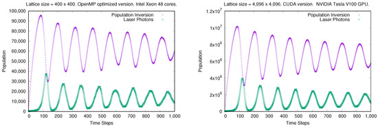
Figure 1.
Output of the model for particular values of the system parameters corresponding to a laser spiking behavior. Parameter values: , , and . The results are smoother for larger lattice sizes. (Left): Parallel OpenMP optimized implementation with a lattice size of cells. (Right): Parallel CUDA implementation with a lattice size of cells.
4.1. Multicore Architecture
The multicore architecture was executed and tested on the two following platforms.
4.1.1. High-End Multicore CPUs (48 Cores)
We evaluated the performance on a high-performance server CPU running in the Cloud, using the Amazon Web Server (AWS) Infrastructure as a Service (IaaS) EC2 service. We ran our performance test on a m5.24xlarge instance. It ran on a dual socket server with 2 Intel Xeon Platinum 8259CL processors with 24 physical cores each (completing 48 physical cores and up to 96 threads between them), running at a frequency of GHz, with MiB of cache memory. The total RAM memory was 373 GiB. Both processor sockets were linked by Ultra Path Interconnect (UPI), a high speed point-to-point interconnect link delivering a transfer speed of up to GT/s.
4.1.2. Consumer-Oriented Multicore CPU (Eight Cores)
The performance was evaluated on a PC with a Core i9 9900 k processor and a total RAM memory of 16 GiB. The processor frequency was GHz and the RAM memory was on a single channel running at 2400 MHz. This processor has eight physical cores, each core supporting two hardware threads (completing a total of 16 Threads).
4.2. GPU Architecture
The following two GPU chips were used to run and test the GPU architecture.
4.2.1. High-End GPU Chip
We evaluated the performance on a p3.2xlarge instance of the Amazon Web Server(AWS) IaaS EC2 Cloud Computing service. It used a NVIDIA Tesla V100 GPU (Volta architecture) with 5120 CUDA cores and a GPU memory of 16 GiB. The server used an Intel Xeon E5-2686v4 CPU with four physical cores running at GHz. CPU and GPU were interconnected via PCI-Express Generation 3, with a bandwidth of 32 GiB/s.
4.2.2. Consumer-Oriented GPU Chip
We used a consumer-oriented NVIDIA GeForce GTX 1050 Ti graphic card (Pascal architecture). This card has 768 CUDA cores running at 1290 MHz. The total memory is 4 GiB of GDDR5 type, with a maximum bandwidth of 1120 GiB/s.
4.3. Performance and Scalability Results
Figure 2 shows the speedup of the parallel OpenMP implementation running on the Core i9 9900 k PC (eight cores). In this case, speedups are fairly foreseeable. Firstly, for small lattice sizes, most of matrices reside in CPU caches, thereby achieving an excellent speedup versus the sequential (one thread) test until eight threads. Launching nine threads implies that a physical CPU must manage two threads (whereas the rest of CPUs, only one), thereby causing the speedup to decrease. However, this problem diminishes for more threads. Finally, Core i9 simultaneous multi-threading begins to play a role from nine threads up; hence, speedups above eight were reached for some tests when launching many threads.
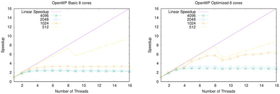
Figure 2.
Speedup of the parallel OpenMP implementation running on a consumer-oriented CPU with eight cores. (Left): Basic implementation without in-depth optimization. (Right): Fully optimized implementation.
In addition, speedups were stuck according to the maximum RAM bandwidth for big lattices, as predicted by the roof-line model [35]. In these cases, RAM memory bandwidth was the bottleneck that in fact determined program runtimes.
In the case of the the high-end server with two Intel Xeon Platinum 8259CL CPUs (see Figure 3), our parallel implementation shows an excellent speedup for large lattice sizes. The OpenMP optimized version reaches a speedup around ×30 for 48 threads. The behaviors were similar to those obtained in the consumer-oriented hardware: a peak on the speedups was reached when launching the same number of threads as physical CPUs; then, accelerations began to decrease with more threads; and finally, speedups were recovered when the number of threads doubled the number of physical cores.
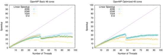
Figure 3.
Speedup of the parallel OpenMP implementation running on a high-end dual-socket server with a total of 48 cores. (Left): Basic implementation without in-depth optimization. (Right): Fully optimized implementation.
Nevertheless, for high number of threads, or more precisely, for small numbers of lattice rows per thread, the computation-to-communication scale began to deteriorate speedups. Note that small lattices (Figure 3 for lattice width ) exhibit this problem, whereas big lattice speedups are almost not deteriorated. This is a well-known effect when scientific applications are massively distributed [36]. Because the CA model studied here involves communication between neighboring cells (using the Moore neighborhood), the more threads in which we divide the lattice, the more communication between threads requires, thereby degrading the parallel performance.
In Figure 4, Figure 5, Figure 6 and Figure 7 we show a runtime comparison between both CPU/GPU pairs, for different sizes and number of multicore threads. It is interesting to note that for CPU/GPU comparisons shown in these figures, CUDA implementation is, at most, 2.5 times faster than the OpenMP Optimized version. In truth, GPU platforms beat clearly CPU ones only for large lattice sizes: as shown in Figure 7, that happens only for a number of threads much smaller than the number of available physical cores of the CPU and for large system sizes. However, when using the 48 available cores of the CPU, the CUDA implementation is again, only around 2.5 times faster than the CPU. Moreover, CPU and GPU runtimes are even similar for small system sizes.
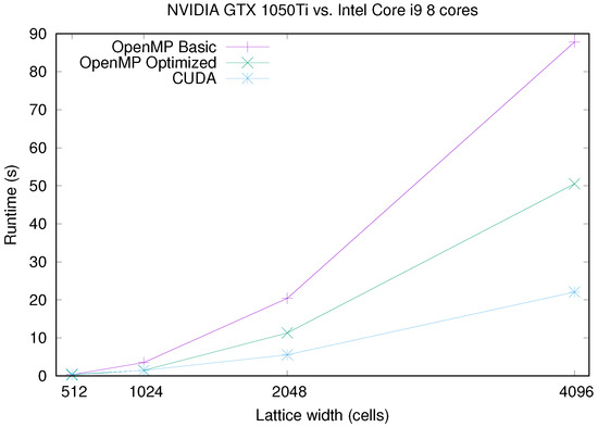
Figure 4.
Runtime comparison between NVIDIA GTX 1050 Ti GPU and Intel Core i9 (eight cores) for different CA lattice sizes.
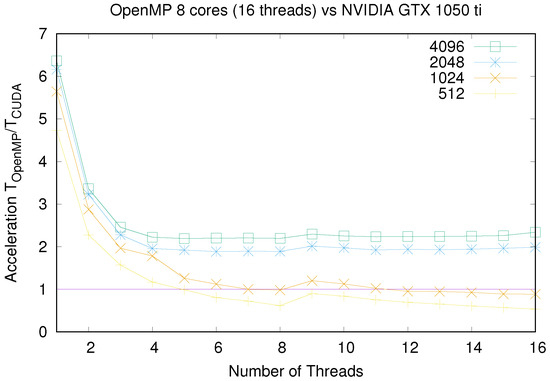
Figure 5.
Comparison of OpenMP Optimized and CUDA times when using Intel Core i9 and NVIDIA GeForce GTX 1050 Ti resp.
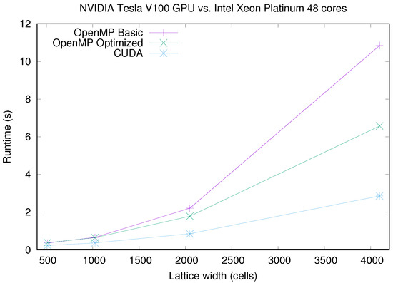
Figure 6.
Runtime comparison between NVIDIA Tesla V100 GPU and Intel Xeon Platinum (dual socket with 48 cores in total) for different CA lattice sizes.
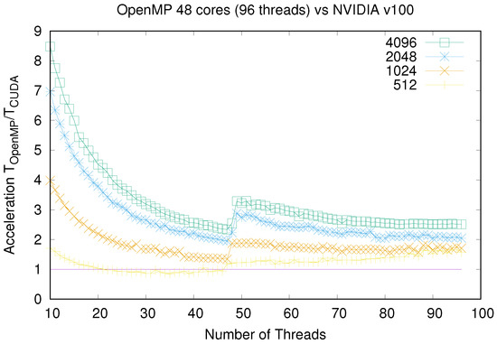
Figure 7.
Comparison of OpenMP Optimized and CUDA times: Detail from 10 threads up when using Intel Xeon Platinum and NVIDIA Tesla V100 GPU, respectively.
An additional consideration plays in favor of classical CPU platforms. If a previously computed random list were used as an input for the model, (thus preventing the time spent in computing random numbers during simulation; see Section 3.3.1), OpenMP Optimized simulation times would be even lower than those of CUDA versions. We recall here that, although this alternative is practical only for medium lattice widths, it speeds up OpenMP version around three times. This optimization does not favor GPU platforms so much.
5. Conclusions and Future Lines
In some previous studies cited in the introduction and Section 2, it was pointed out that the speedups achieved with GPU when comparing to single-core CPUs where above ×10 and sometimes above ×100. Even with these ratios, it is evident that a current multicore CPU may approach GPU performance. Moreover, this affirmation must be revised and carefully analyzed for Cellular Automata (CA) applications. In this paper, it was experimentally proven, using almost the same code for a laser dynamics CA (except for the necessary adaptation to each platform), that these distances were significantly shortened. We conclude that nested conditional structures (in general, many branches in the "hot spot" zones) imply that GPU implementations would suffer from an important deceleration. As a result, in spite of CA being massivelly parallel data structures, less than a ×3 speedup can be achieved for GPUs against high performance CPUs. The other factor that limits CPU and GPU performance for big lattice CAs is obviously the maximum RAM bandwidth, as predicted by the roofline model. If other variables were taken into account, such as price, TDP, source code maintenance, or easy and rapid software development, it is not clear that GPUs are always the best choice for an efficient parallelization of CA algorithms.
Future lines, provided the important conclusions obtained in this paper for the specific case of laser dynamics, include the extension of this analysis to generic cellular automata. This will be necessary in order to extract a simple but realistic model that allows one to predict the performance on CPU and GPU platforms mainly as a function of the form of its state transition rules, its neighboring relations, the amount of memory, etc. It will be also interesting to investigate the efficient implementation and speedup obtained by implementing this model on multi-GPUs.
Another interesting line to be investigated concerns speeding up the simulation by substituting the pseudorandom number generator by a different type of algorithm that can be faster. A good alternative can be an algorithm that generates pseudorandom numbers based on the calculation of chaotic sequences, such as those presented in [37,38]. Those results suggest that they could reduce the execution overhead, and thus contribute to a further speedup of the implementation of the studied laser CA model.
Author Contributions
Conceptualization, D.C.-M., F.D.-d.R., and J.L.G.; methodology, D.C.-M., F.D.-d.R., M.R.L.-T., and J.L.G.; software, D.C.-M., F.D.-d.R., M.R.L.-T., and J.L.G.; validation, D.C.-M., F.D.-d.R., and J.L.G.; investigation, D.C.-M., F.D.-d.R., F.J,. and J.L.G.; resources, D.C.-M., F.D.-d.R., and J.L.G.; writing—original draft preparation, D.C.-M., F.D.-d.R., F.J.-M., and J.L.G.; writing—review and editing, D.C.-M., F.D.-d.R., and J.L.G.; visualization, D.C.-M. and M.R.L.-T.; supervision, J.L.G.; funding acquisition, D.C.-M., F.J.-M., and J.L.G. All authors have read and agreed to the published version of the manuscript.
Funding
This research was funded by the following research project of Ministerio de Economía, Industria y Competitividad, Gobierno de España (MINECO), and the Agencia Estatal de Investigación (AEI) of Spain, cofinanced by FEDER funds (EU): MABICAP (Bio-inspired machines on High Performance Computing platforms: a multidisciplinary approach, TIN2017-89842P). The work was also partially supported by the computing facilities of Extremadura Research Centre for Advanced Technologies (CETA-CIEMAT), funded by the European Regional Development Fund (ERDF). CETA-CIEMAT belongs to CIEMAT and the Government of Spain.
Conflicts of Interest
The authors declare no conflict of interest. The funders had no role in the design of the study; in the collection, analyses, or interpretation of data; in the writing of the manuscript, or in the decision to publish the results.
References
- Talia, D.; Naumov, N. Parallel cellular programming for emergent computation. In Simulating Complex Systems by Cellular Automata; Springer: Berlin/Heidelberg, Germany, 2010; pp. 357–384. [Google Scholar]
- Bandini, S.; Mauri, G.; Serra, R. Cellular automata: From a theoretical parallel computational model to its application to complex systems. Parallel Comput. 2001, 27, 539–553. [Google Scholar] [CrossRef]
- Wolfram, S. Cellular Automata and Complexity; Addison-Wesley: Reading, MA, USA, 1994. [Google Scholar]
- Ilachinski, A. Cellular Automata: A Discrete Universe; World Scientific: Singapore, 2001; p. 808. [Google Scholar]
- Sayama, H. Introduction to the Modeling and Analysis of Complex Systems; Open SUNY Textbooks. 14: Geneseo, NY, USA, 2015. [Google Scholar]
- Chopard, B.; Droz, M. Cellular Automata Modeling of Physical Systems; Cambridge University Press: Cambridge, MA, USA, 1998. [Google Scholar]
- Sloot, P.; Hoekstra, A. Modeling Dynamic Systems with Cellular Automata. In Handbook of Dynamic System Modeling; Fishwick, P., Ed.; Chapman & Hall/CRC: London, UK, 2007. [Google Scholar]
- Hoekstra, A.G.; Kroc, J.; Sloot, P.M. (Eds.) Simulating Complex Systems by Cellular Automata; Springer: Berlin/Heidelberg, Germany, 2010. [Google Scholar]
- Gounaridis, D.; Chorianopoulos, I.; Koukoulas, S. Exploring prospective urban growth trends under different economic outlooks and land-use planning scenarios: The case of Athens. Appl. Geogr. 2018, 90, 134–144. [Google Scholar] [CrossRef]
- Aburas, M.M.; Ho, Y.M.; Ramli, M.F.; Ash’aari, Z.H. The simulation and prediction of spatio-temporal urban growth trends using cellular automata models: A review. Int. J. Appl. Earth Obs. Geoinf. 2016, 52, 380–389. [Google Scholar] [CrossRef]
- Liu, X.; Liang, X.; Li, X.; Xu, X.; Ou, J.; Chen, Y.; Li, S.; Wang, S.; Pei, F. A future land use simulation model (FLUS) for simulating multiple land use scenarios by coupling human and natural effects. Landsc. Urban Plan. 2017, 168, 94–116. [Google Scholar] [CrossRef]
- Qiang, S.; Jia, B.; Huang, Q.; Jiang, R. Simulation of free boarding process using a cellular automaton model for passenger dynamics. Nonlinear Dyn. 2018. [Google Scholar] [CrossRef]
- Tang, T.Q.; Luo, X.F.; Zhang, J.; Chen, L. Modeling electric bicycle’s lane-changing and retrograde behaviors. Phys. A Stat. Mech. Its Appl. 2018, 490, 1377–1386. [Google Scholar] [CrossRef]
- Monteagudo, A.; Santos, J. Treatment Analysis in a Cancer Stem Cell Context Using a Tumor Growth Model Based on Cellular Automata. PLoS ONE 2015, 10, e0132306. [Google Scholar] [CrossRef]
- Burkhead, E.; Hawkins, J. A cellular automata model of Ebola virus dynamics. Phys. A Stat. Mech. Appl. 2015, 438, 424–435. [Google Scholar] [CrossRef]
- Guisado, J.; Jiménez-Morales, F.; Guerra, J. Cellular automaton model for the simulation of laser dynamics. Phys. Rev. E 2003, 67, 66708. [Google Scholar] [CrossRef]
- Guisado, J.; Jiménez-Morales, F.; Guerra, J. Computational simulation of laser dynamics as a cooperative phenomenon. Phys. Scr. 2005, T118, 148–152. [Google Scholar] [CrossRef]
- Guisado, J.; Jiménez-Morales, F.; Guerra, J. Simulation of the dynamics of pulsed pumped lasers based on cellular automata. Lect. Notes Comput. Sci. 2004, 3305, 278–285. [Google Scholar]
- Kroc, J.; Jimenez-Morales, F.; Guisado, J.L.; Lemos, M.C.; Tkac, J. Building Efficient Computational Cellular Automata Models of Complex Systems: Background, Applications, Results, Software, and Pathologies. Adv. Complex Syst. 2019, 22, 1950013. [Google Scholar] [CrossRef]
- Guisado, J.; Fernández-de Vega, F.; Jiménez-Morales, F.; Iskra, K. Parallel implementation of a cellular automaton model for the simulation of laser dynamics. Lect. Notes Comput. Sci. 2006, 3993, 281–288. [Google Scholar] [CrossRef]
- Guisado, J.; Jiménez-Morales, F.; Fernández-de Vega, F. Cellular automata and cluster computing: An application to the simulation of laser dynamics. Adv. Complex Syst. 2007, 10, 167–190. [Google Scholar] [CrossRef]
- Guisado, J.; Fernandez-de Vega, F.; Iskra, K. Performance analysis of a parallel discrete model for the simulation of laser dynamics. In Proceedings of the International Conference on Parallel Processing Workshops, Columbus, OH, USA, 14–18 August 2006; pp. 93–99. [Google Scholar]
- Guisado, J.; Fernández de Vega, F.; Jiménez-Morales, F.; Iskra, K.; Sloot, P. Using cellular automata for parallel simulation of laser dynamics with dynamic load balancing. Int. J. High Perform. Syst. Archit. 2008, 1, 251–259. [Google Scholar] [CrossRef]
- GPGPU. General-Purpose Computation on Graphics Hardware. Available online: https://web.archive.org/web/20181109070804/http://gpgpu.org/ (accessed on 9 November 2018).
- Lopez-Torres, M.; Guisado, J.; Jimenez-Morales, F.; Diaz-del Rio, F. GPU-based cellular automata simulations of laser dynamics. In Proceedings of the XXIII Jornadas de Paralelismo, Elche, Spain, 19–21 September 2012; pp. 261–266. [Google Scholar]
- Gobron, S.; Devillard, F.; Heit, B. Retina simulation using cellular automata and GPU programming. Mach. Vis. Appl. J. 2007, 18, 331–342. [Google Scholar] [CrossRef]
- Rybacki, S.; Himmelspach, J.; Uhrmacher, A. Experiments With Single Core, Multi Core, and GPU-based Computation of Cellular Automata. In Proceedings of the 2009 First International Conference on Advances in System Simulation, Porto, Portugal, 20–25 September 2009. [Google Scholar]
- Bajzát, T.; Hajnal, E. Cell Automaton Modelling Algorithms: Implementation and Testing in GPU Systems. In Proceedings of the 2011 15th IEEE International Conference on Intelligent Engineering Systems, Poprad, Slovakia, 23–25 June 2011. [Google Scholar]
- Balasalle, J.; Lopez, M.; Rutherford, M. Optimizing Memory Access Patterns for Cellular Automata on GPUs. In GPU Computing Gems Jade Edition; Elsevier: Burlington, MA, USA, 2011; pp. 67–75. [Google Scholar]
- Geist, R.; Westall, J. Lattice-Boltzmann Lighting Models. In GPU Computing Gems, Emerald Edition; Elsevier: Burlington, MA, USA, 2011; pp. 381–399. [Google Scholar]
- Gibson, M.J.; Keedwell, E.C.; Savić, D.A. An investigation of the efficient implementation of cellular automata on multi-core CPU and GPU hardware. J. Parallel Distrib. Comput. 2015, 77, 11–25. [Google Scholar] [CrossRef]
- Jongerius, R.; Anghel, A.; Dittmann, G. Analytic Multi-Core Processor Model for Fast Design-Space Exploration. IEEE Trans. Comput. 2018, 67, 755–770. [Google Scholar] [CrossRef]
- NVIDIA. CUDA C Best Practices Guide Version. Available online: http://developer.nvidia.com/ (accessed on 10 December 2019).
- O’Neill, M.E. PCG: A Family of Simple Fast Space-Efficient Statistically Good Algorithms for Random Number Generation; Technical Report HMC-CS-2014-0905; Harvey Mudd College: Claremont, CA, USA, 2014. [Google Scholar]
- Williams, S.; Waterman, A.; Patterson, D. Roofline: An insightful visual performance model for multicore architectures. Commun. ACM 2009, 52, 65–76. [Google Scholar] [CrossRef]
- Hennessy, J.; Patterson, D. Computer Architecture: A Quantitative Approach, 6th ed.; Elsevier: Burlington, MA, USA, 2017; Volume 19. [Google Scholar]
- Guyeux, C.; Couturier, R.; Héam, P.C.; Bahi, J.M. Efficient and cryptographically secure generation of chaotic pseudorandom numbers on GPU. J. Supercomput. 2015, 71, 3877–3903. [Google Scholar] [CrossRef]
- Wang, L.; Cheng, H. Pseudo-Random Number Generator Based on Logistic Chaotic System. Entropy 2019, 21, 960. [Google Scholar] [CrossRef]
© 2020 by the authors. Licensee MDPI, Basel, Switzerland. This article is an open access article distributed under the terms and conditions of the Creative Commons Attribution (CC BY) license (http://creativecommons.org/licenses/by/4.0/).