Posit Arithmetic Hardware Implementations with The Minimum Cost Divider and SquareRoot


1
School of Microelectronics, Xi’an Jiaotong University, Xi’an 710049, China
2
Faculty of Science in Mechatronic Systems, The University of Melbourne, Melbourne, VIC 3010, Australia
*
Authors to whom correspondence should be addressed.
Electronics 2020, 9(10), 1622; https://doi.org/10.3390/electronics9101622
Submission received: 12 September 2020
/
Revised: 28 September 2020
/
Accepted: 29 September 2020
/
Published: 2 October 2020
(This article belongs to the Special Issue Application of Electronic Devices on Intelligent System)
Abstract
:As a substitute for the IEEE 754-2008 floating-point standard, Posit, a new kind of number system for floating-point numbers, was put forward recently. Hitherto, some studies have proven that Posit is a better floating-point style than IEEE 754-2008 in some fields. However, most of these studies presented the advantages of Posit from the arithmetical aspect, but none of them suggested it had a better hardware implementation than that of IEEE 754-2008. In this paper, we propose several hardware implementations that contain the Posit adder/subtractor, multiplier, divider, and square root. Our goal is to achieve an arbitrary Posit format and exploit the minimum circuit area, which is required in embedded devices. To implement the minimum circuit area for the divider and square root, the alternating addition and subtraction method is used rather than the Newton–Raphson method. Compared with other works, the area of our divider is about 0.2×–0.7× (FPGA). Furthermore, this paper provides the synthesis results for each critical module with the Xilinx Virtex-7 FPGA VC709 platform.
Keywords:
Posit; IEEE 754-2008; FPGA; floating-point arithmetic; adder; multiplier; divider; square root1. Introduction
In 2015, a new kind of number system named the universal number (Unum) system was put forward by some researchers. Unum has developed three revisions so far. They are Type-1 [1,2,3], Type-2 [4,5], and Type-3 [6,7]. The latest revision was Type-3 and also called Posit. The developers of Unum claimed that Unum was used to replace the IEEE 754-2008 floating-point standard [8] with more efficiency and high precision. Comparing with IEEE 754-2008, both Unum and Posit have many advantages such as a better dynamic range, higher coding space utilization, tapered accuracy, parameterized precision, and so on [6].
Posit arouses the interest of many researchers in the community. As a result, there are many studies on exploiting the advantages of Posit from the arithmetical aspect. Meanwhile, there are many software tools for using Posit such as Julia, C, C++, and so on. Reference [9] conducted a thorough investigation on training deep neural networks (DNNs) with low bit posit numbers, a Type-III Unum. Through a comprehensive analysis of quantization with various data formats, it is demonstrated that the posit format shows great potential to be employed in the training of DNNs. To propagate Posit and replace IEEE 754-2008 in some fields such as deep learning, it is better to design an excellent Posit processing unit (PPU) for microprocessors because Posit is more accurate near zero. There are some open-source hardware implementations. This paper aims to exploit a basic arithmetical processor for Posit, including adder/subtractor, multiplier, divider, and square root. Before introducing these modules, let us go through a brief background of Posit in this section.
The format of Posit is flexible since its word width and exponent width are arbitrary. Unlike only the four formats that the IEEE 754-2008 standard defined, the format of Posit can be adjusted freely according to the users’ needs. By adjusting the format, Posit has a suitable precision and dynamic range for different applications.
The precision of Posit is tapered since its sampling density function on the real axis is not linear [10]. The integration of the sampling density function is the cumulative density function. Interestingly, the cumulative density function of Posit is the sigmoid function, which is often used as the activation function in deep learning. It is easy to get the sigmoid function by left shifting Posit [6]. These two functions are presented in (1). Most parts of the coding space of Posit fall in the range from −1 to one. In deep learning, most network weights also fall in this range. Reference [11] proved that Posit is better than IEEE 754-2008 floating-point numbers in the deep learning field.
The coding style of Posit is elegant in mathematics. There is only one kind of bit pattern for zero, and the encoding is symmetric around one. In addition, the hidden bit of Posit is always one. On the contrary, the IEEE 754-2008 standard defines positive zero and negative zero, which are different and have different behaviors. To underflow gradually, the IEEE 754-2008 standard defines two hidden bits, which are one and zero. This means that the calculation of Posit is more accurate and simpler.
Posit makes good use of coding space since no bit patterns are redundant. There are only two abnormal cases in Posit. One of them is zero, and the other is NaR (not a real number). If all bits of a Posit number excluding the most-significant bit (MSB) are zero, it is NaR. If the MSB is also zero, it is zero. Otherwise, the Posit number is a normal case. As IEEE 754-2008 defines, there are many invalid bit patterns for NaN (not a number). NaN has an adverse effect on calculation, which makes the circuit complex. NaR is not identical to NaN. NaR means it is a number, but not a real number. For example, the square root of −1 is i, which is an imaginary number that NaR can represent. NaN is produced by uninitiated memories or exceptional operations.
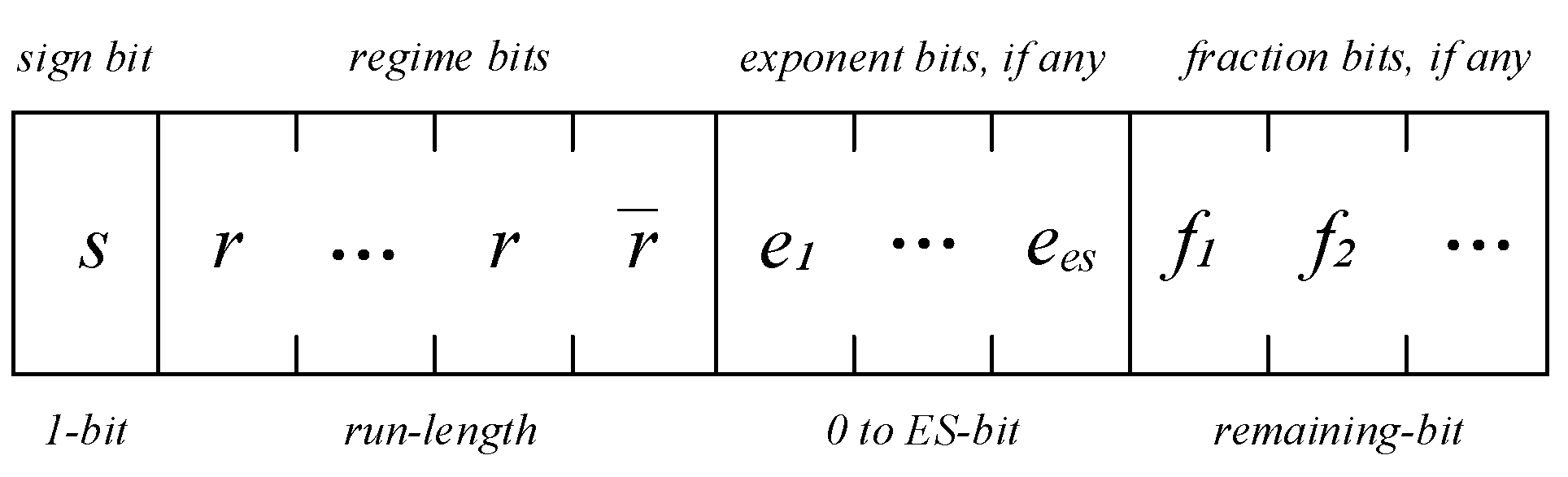
A normal Posit number is illustrated in Figure 1. The MSB is its sign bit. If a normal Posit number is positive, the MSB is zero; otherwise, it is one. The field next to the sign bit is called the regime. Presuming the word width of Posit is N, the minimum width of the regime is two, and the maximum width is . The regime is leading ones or leading zeros, and its value is represented by the run length of these bits. If the number of leading bits of leading ones is R, the value of the regime is . Replacing the leading ones with leading zeros, the value will be . Table 1 shows the relationship between the value of the regime and the leading bits.
The exponent field will be demonstrated after the regime field if any bits remain. The exponent field is an unsigned integer. Its maximum width includes a predetermined constant and the factor of a variable named useed. Presume its maximum width is the exponent width (ES) and the value of useed is determined by (2). The final field is the fraction, and it occupies all the remaining bits.
The value of a normal Posit number can be calculated by (3). Because the regime is the exponent of useed, the actual exponent of Posit consists of the regime and exponent field. In other words, the actual exponent is , and the base number is two. This feature makes values with small exponents have more digits of accuracy, and values with large exponents have fewer digits of accuracy.
Posit<5, 1> means that the word width of Posit is five and the exponent width is one. Combining with (3), the maximum positive value of Posit<5, 1> is 64, and its bit pattern is . This value is also called the maxpos. Similarly, the minposis , and its bit pattern is . An important feature of Posit is that it is encoded in the two’s complement. That is, inverting all bits of a Posit number and adding one will get its opposite number. For example, the opposite number of is , i.e., −minpos.
The calculating rules are simple. If one of the inputs is NaR or the operation is illegal, the output must be NaR. Otherwise, the output must be zero or a normal number. The solution of overflow and underflow is saturating the output. Specifically, if a positive output is greater than the maxpos or less than the minpos, the output is trimmed to the maxpos or increased to the minpos, respectively. Furthermore, a negative output must be from −maxpos to −minpos. The rules of rounding are also simple. There is only one rounding mode, i.e., rounding the result to the nearest value. However, IEEE 754-2008 defines many rounding modes. These modes make hardware implementations more complex.
Ultimately, Posit is a novel number system that is better than the IEEE 754-2008 floating-point number standard in some fields. It is flexible, simple, elegant, and accurate. Above all, the hardware implementation of Posit is simpler than that of IEEE 754-2008 in theory.
2. Related Works
Because of the superiority of Posit, there have been several hardware implementations of Posit. A parameterized adder/subtractor was presented in [12]. Similar to [12], a parameterized adder/subtractor and a parameterized multiplier were presented in [13]. These two works used both the leading ones detector (LOD) and leading zeros detector (LZD) to determine leading bits. To process negative Posit numbers, these two works converted negative Posit numbers to the corresponding opposite numbers. Although their algorithms are simple, the hardware implementations are not ideal. They have two obvious shortcomings, i.e., both LOD and LZD produce redundant area while converting the two’s complement to sign and magnitude.
Another work exhibited in [14] solved the first shortcoming. In its algorithm, only LZD is used. Unfortunately, the second shortcoming still exists, and this work cannot make good use of the advantages of Posit. Based on this work, Reference [15] indicated a parameterized divider with the Newton–Raphson method.
Reference [11] not only studied the applications of Posit in software, but also gave a simple hardware implementation. This implementation encodes Posit in sign and magnitude. This smart solution simplifies circuits, but does not conform to the Posit standard.
Our work solves those two problems so that our implementation cost is small and gives a complete solution for Posit arithmetic.
3. Critical Common Modules
Due to the length of the regime field being floating, firstly, a Posit number must be decoded to get its sign, exponent, and mantissa. Then, these three fields will be used to calculate and encode the final Posit number. In a word, encoding and decoding are common stages in every Posit algorithm. Figure 2 shows these three stages of a general Posit arithmetic flow.
Using both LOD and LZD is a normal method for extracting the regime field in the decoding stage and normalizing the mantissa in the calculation stage. However, our work only needs LZD. Unlike other studies that only use normal LZD, the advanced LZD is used instead, which saves much of the area when the width of the input is large. According to the synthesis results, the implementations that only use LZD save about 5–10% of the area compared with those who use both LOD and LZD.
In this section, firstly, the advanced LZD is introduced. Secondly, two outstanding common modules, the encoding module and the decoding module, are explained. The following is the design ideas for the encoding module, the decoding module, and the LZD module.
3.1. The Optimization for LZD
Usually, LZD outputs a binary number to represent how many consecutive zeros from the start-end to the first inverse bit of the input. For instance, inputting will get (). An N bit input will produce an L(N) bit result. Equation (4) illustrates the way to calculate L(N).
There are two kinds of zero sequence detectors in Figure 3, the shift comparison (left) and the direct comparison (right). The direct comparison takes up fewer resources because the bit width to be compared is shorter.
3.2. The United Intermediate Data Structure
To unify the interfaces among every stage, a kind of intermediate data structure is defined. This data structure is the intermediate result in Figure 2. This intermediate data structure has six fields. Table 2 lists all these fields and describes their meanings. Given that the word width of Posit is N and the exponent width is ES, the maximum width of the regime is , and the width of its value can be calculated with (4). Furthermore, the value of the regime needs one more bit as a sign bit. Therefore, the width of the scale field is . The maximum width of the fraction is because the whole Posit needs to remove a 1 bit sign, 2 bit regime, which is the minimum width itself and the ES bit exponent.
3.3. The Decoding Module
The decoding module extracts an intermediate data structure from an input Posit number, and this structure is used to calculate the result. The two’s complement is usually used in arithmetic since the sign of the result is produced easily. As mentioned earlier, one of the advantages of Posit is that its coding format has the two’s complement. If the output of the decoding module keeps the two’s complement format, the calculation module will be simpler since it does not need extra logic to deal with the sign and case of overflow. However, the related works [12,13,14,15] did not keep this advantage. They converted the Posit numbers to sign and magnitude so that the decoding logic would be simpler. Our work still uses the two’s complement.
As presented in Algorithm 1, the intermediate data structure is extracted from an input Posit number without a conversion operation. Its explanation is as follows:
- In positive Posit numbers, leading ones represent a positive regime, and leading zeros represent a negative regime. The negative Posit numbers are opposite since they are the two’s complement. A simple way to determine this is by using an XOR operation between in [N−1] and in [N−2]. The rSign field stands a positive regime when it is one (Line 7).
- To use LZD solely to detect the regime, use an XOR operation between the regime and itself so that leading ones become leading zeros and leading zeros stay the same. Apart from this, one of the inputs of this operation must be left-shifted by 1 bit, which will produces the end bit for the result. For instance, presume a regime is and an XOR operation between and will produce . This is the reason for using an XOR operation between in [N−2:1] and in [N−3:0]. The potential exponent and fraction do not change the position of the end bit. Therefore, this operation contains the possible maximum width of the regime. The result of this operation is input to an ILZD module (inverting the final output of LZD) (Lines 8–9).
- All bits of the output of ILZD are inverted from those of LZD. On the one hand, the output of LZD is the actual value of leading zeros, and it must be a non-negative number. On the other hand, to represent a negative regime, the output of LZD should be inverted, plus one, and extended with a 1 bit sign. Therefore, the output of ILZD is inverted when the regime is positive; otherwise, the output of ILZD stays the same. In addition, the rSign field is the sign bit of the regime. The length of leading zeros produced in the previous step is 1 bit less than the original length. Occasionally, the value of a positive regime is one less than the length of leading bits. From the point of view of the two’s complement, inverting all bits without adding one means taking a positive number to negative and subtracting one. That means the sReg field represents the proper value for the regime in the two’s complement (Lines 10–11).
- The rLength field is one less than the original length. For the reduced one, the solution is to remove the three most-significant bits from the original input since equal the length of the regime with a sign bit. Then, left shifting in [N−4:0] by rLength bit and the original input will leave the exponent and fraction only, i.e., the expFrac field. This method avoids the use of one additional adder and reduces the input width of the shift circuit (Lines 12–13).
- If all bits of the input are zero except the MSB, the input is NaR. If the MSB is also zero, the input is zero. Otherwise, the input is a normal number, and its sign bit is the MSB (Lines 14–16).
- If ES is larger than zero, the ES most-significant bits of expFrac are the exponent, and the others are the fraction. Note that a negative Posit number should invert its exponent. The scale field is produced by concatenating the value of the regime and the exponent. If ES is zero, the scale field is the value of the regime. Since the decoder does not have any right shift logic, the grs field is zero (Lines 17–25).
To get the bit pattern of a negative Posit number, the corresponding positive Posit number will invert all bits plus one. If every bit of the fraction is zero, inverting them plus one will give the exponent a carry bit. One problem is that this carry bit will change the exponent. For example, a positive Posit number is 0_110_11_00, and its opposite number is 1_001_01_00. In Algorithm 1, a negative Posit number will invert its exponent so that the exponent is (). Its actual exponent should be (). That is to say, the scale produced by Algorithm 1 is one less than the actual scale when all bits of the fraction of a negative Posit number are zero. Likewise, the regime will be one less than the actual regime if its exponent is also zero or does not exist. Therefore, the final scale is one less than the actual scale.
Another method is used to fix this problem. In the calculation stage, the mantissa encoded in the two’s complement consists of the sign bit, hidden bit, and fraction. For the positive mantissas, the sign bit is zero, and the hidden bit is one. The negative mantissas, except −1.0, are the opposite. Therefore, a mantissa being used to calculate can be constructed with (5). Because the fraction of a negative Posit number has been inverted plus one, this mantissa is the two’s complement. If all bits of the fraction of a negative number are zero, the mantissa should have been (), but (5) gives (). Coincidentally, this offsets the problem that the scale produced by Algorithm 1 is one less than the actual scale.
Expression (6) sums up the range of the mantissa produced by our decoder. Note that all inputs of the calculation module fall within this range. All outputs of the calculation module must also fall within this range.
| Algorithm 1: The Posit decoder. |
 |
3.4. The Encoding Module
As the encoding module is the inverse process of the decoding module, its input is an intermediate data structure, and its output is a Posit number. Compared to the decoder, the encoder focuses on rounding the Posit number. Algorithm 2 describes the details of the encoder, and its explanation is as follows:
- Extract the value and sign of the regime and the exponent from the scale field. The end bit of the regime requires a 1 bit XOR operation between the sign field and the sign of the regime. The end bit is inverted to get the start bit. Concatenate the start bit, end bit, exponent, fraction, and grs to get the refg (regime, exponent, fraction, and grs) field. Arithmetical right shifting refg by the rLength bit will produce proper leading bits as the regime (Line 7–17).
- The four least-significant bits are the last bit of the Posit number, guard bit, round bit, and sticky bit, respectively. In the IEEE 754-2008 standard, the result will add one if GRSis larger than or GRS equals , and the last bit is one. This work also takes this principle. Apart from this, the Posit standard requires the result, which cannot be rounded to zero or NaR. If all bits of result [N+1:3] are zero, concatenating it and the sign field will get (zero) or (NaR), so the result must add one. On the contrary, the result should not add one if all bits are one. If the result is not either of these cases, round it by GRS (Lines 18–26).
- If the isNaR field is true, the output must be (NaR). If the isZero field is true, the output must be (zero). Otherwise, the output is produced by concatenating the sign field and rounded result. Note that isNaR and isZero cannot be true simultaneously, and the other four fields are invalid if one of these two fields is true (Lines 27–33).
| Algorithm 2: The Posit encoder. |
 |
3.5. The Posit Divider and Square Root Core
Using the Newton–Raphson method, we can design a fast divider, but the cost is the large area and high power. The alternating addition and subtraction method is the opposite. According to the synthesis results, the area and power produced by the alternating addition and subtraction method are approximately equal to those of the Posit adder. The drawback of this method is low speed because it produces only one bit of the result every clock period. Using LUTs to construct the Posit divider is more sensible when the input width is small such as 8 bit.
The prerequisite of this method is that the absolute value of the dividend must be less than that of the divisor. This ensures that the quotient must be a negative number when two inputs have different signs. To achieve this, two mantissas are constructed with (5). Then, the dividend is extended with a 2 bit sign more, and the divisor is multiplied by four. The range of the temporary quotient is (−1, 1), and its binary point follows the MSB. To restore the result, the binary point can be considered to follow the third-significant bit. The actual range of the mantissa of the quotient is presented in (7).
All bits of the quotient are initialized to zero. Each bit from the MSB to the LSB is produced in each clock period. In the first iteration, the dividend should subtract or add the divisor if their signs are the same or different, respectively. Then, if the remainder has the same sign bit as the divisor, the MSB of the quotient should be one; otherwise, it should be zero. Update the dividend with the remainder if the dividend, i.e., the last remainder, is not zero.
In the second iteration, firstly, the new dividend should be left-shifted by 1 bit. Then, it should subtract or add the divisor if their signs are the same or different, respectively. If the new remainder is zero, the second-significant bit of the quotient should be the opposite of the MSB. Otherwise, this bit is zero or one when the new remainder has a different or the same sign bit from or as the divisor, respectively. Furthermore, update the dividend with the new remainder when the dividend is not zero. Specifically, if the dividend is zero, the currently calculated bit of the quotient remains the same as the MSB, and the dividend does not need to be updated, which means the division is complete.
Repeat the second iteration several times until sufficient bits are produced. Finally, the result should add its sign bit because it is the one’s complement. Table 3 gives the decimal values, scale biases, and final bit patterns for all quotients. If the MSB and the third-significant bit of the bit pattern are the same, the scale bias is negative. Based on that, the scale bias is −2 only if the MSB and the fourth-significant bit are the same.
The alternating addition and subtraction method can be used to extract the square root. In each iteration, the square value of the intermediate square root is compared with the original input. If the square value is still less than the original input, the currently calculated bit is one; otherwise, it must be zero.
In particular, if the square value equals the original input, the currently calculated bit is one, and the remaining bits are zero since the calculation is complete.
If the scale of the input is even, the scale of the result is just half of it. If not, the scale should subtract one, and the mantissa should left shift by 1 bit. Combining with (6), the range of the mantissa of the square root is shown in (8).
Algorithm 3 gives all the iterations in mathematics. According to (8), , the result of the first iteration, must be one. Next, the keynote is the equation written in Line 16. It will implement the coefficient of , i.e., , that left shifts by 1 bit in each iteration. Then, the result should set the current calculation bit to one. Compare and and confirm whether the current calculation bit is one or zero. After iterating times, the intermediate result is the final output.
The Posit divider and the Posit square root have something in common. Firstly, their remainders both need to be left-shifted by 1 bit in each iteration. Secondly, the Posit square root needs a “divisor” to assist the calculation. Thirdly, the currently calculated bits of these two modules are both produced by comparing the signs of the dividend and divisor. Ultimately, their current operations are both determined with the signs of the dividend and divisor.
| Algorithm 3: The iteration process of the square root. |
 |
As Algorithm 4 presents, the division and square root can be solved with the same module. A keynote is constructing the “divisor” for extracting the square root (Line 61). This “divisor” is a variable. As mentioned earlier, the binary point of the dividend follows the fourth-significant bit, and that of the intermediate result follows the third-significant bit. That means implementing does not require any operation for the intermediate result. Right-shifting bitMask by 1 bit will get the currently calculated bit. If the current dividend is negative, i.e., is negative in the last iteration, it must add a complement after left-shifting. The complement is . Furthermore, the current dividend should subtract the current divisor, which is . Combining the complement and current divisor, the actual divisor is since is just .
| Algorithm 4: The Posit divider and square root core. |
   |
4. Implementation Results
All our algorithms were functionally verified against the open-source C++ program, which is available at [16]. Furthermore, all RTL codes were implemented on FPGA platforms. The FPGA platform was Xilinx Virtex-7 FPGA VC709, and the development tool was Vivado 2020.01. The synthesis and implementation strategy was set to the Vivado default settings. The option, max_dsp, must be set to zero, since using LUTs solely can get a more accurate comparison. Posit<N, 1> was selected for comparison because PAC and HDL do not support Posit<N, 0>. The Posit<N, es> results in other cases were similar to Posit<N,1>.
Two open-source implementations for Posit, PositHDL and PACoGen, are indicated in [17,18], respectively. Compared with them, the greatest improvement of this work is in the multiplier maximum net delay and divider resource utilization. The adder resource utilization and maximum net delay are better than PACoGen, but worse than PositHDL, both in LUTs and delay. The multiplier is only better than the two works in terms of delay by a difference of 3ns in the best case (at N = 20). The implementation of these three works with the above conditions and the results are summarized in Figure 4, Figure 5 and Figure 6. To measure the timing, all inputs and outputs are connected to the registers since these modules are the combination logic. Nevertheless, these extra registers are not counted in the area.
The adder and multiplier comparison with [14] on a Zedboard with a Zynq-7000 SoC is given in Table 4. Our LUTs and delay are better than [14] when the bit configuration is Posit<16, 1>. The LUTs are very close, but our delay is about 2ns better than [14] when the bit configuration is Posit<32, 1>.
PositHDL and [14] does not implement the Posit divider. The cost of the Posit divider of PACoGen is very high since it is based on the Newton–Raphson method. Our divider and square root are based on the alternating addition and subtraction method, so it takes N clock cycles to complete an operation with Nbits. Compared with PACoGen, the cost of our work is much lower, and our Posit divider is better in area (0.2×–0.7×); however, the calculation time is 3.1 (at N = 19) to 4.9 (at N = 32) times longer.
5. Conclusions
Recently, a new floating-point standard named Posit has become a popular study topic. The Posit standard has shown some advantages over the IEEE 754-2008 standard.
This paper puts forward a series of new algorithms for the Posit adder/subtractor, multiplier, divider, and square root. Besides, the most critical improvement is the redesign of two submodules, i.e., the decoding module and encoding module. All algorithms of this paper can be applied to any word width (N) and exponent width (ES) combination and comply fully with the Posit standard. This work will enable more researchers to exploit more advanced designs and promote the application of Posit in low-power devices. Finally, this paper provides the data of our work on the Xilinx Virtex-7 FPGA VC709 platform. These data prove that our work is better than other works in multiplier delay, divider resource utilization, and square root resource utilization. Our adder and multiplier resource utilization is not the best because our LZD is not excellent. We will design the LZD based on this dichotomy to improve it in the future.
Author Contributions
Conceptualization, F.L. and G.Z.; methodology, B.W.; software, B.W.; validation, F.X., J.L. and S.C.; formal analysis, G.Z.; investigation, S.C.; resources, Z.L.; data curation, F.X.; writing—original draft preparation, Z.L.; writing—review and editing, F.X.; visualization, S.C.; supervision, F.L.; project administration, F.L.; funding acquisition, F.L. All authors have read and agreed to the published version of the manuscript.
Funding
This work was supported by the National Natural Science Foundation of China (No. 61474093) and the Natural Science Foundation of Shaanxi Province, China (No. 2020JM-006).
Conflicts of Interest
The authors declare no conflict of interest. The funders had no role in the design of the study; in the collection, analyses, or interpretation of data; in the writing of the manuscript; nor in the decision to publish the results.
References
- Gustafson, J.L. The End of Error: Unum Computing, 1st ed.; CRC Press: Boca Raton, FL, USA, 2015. [Google Scholar]
- Tichy, W. The end of (numeric) error: An interview with John L. Gustafson. Ubiquity 2016, 2016, 1. [Google Scholar] [CrossRef] [Green Version]
- Brueckner, R. Slidecast: John Gustafson Explains Energy Efficient Unum Computing. Inside HPC. 2015. Available online: https://insidehpc.com/2015/03/slidecast-john-gustafson-explains-energy-efficient-unum-computing/ (accessed on 13 March 2019).
- Gustafson, J. A radical approach to computation with real numbers. Supercomput. Front. Innov. 2016, 3, 38–53. [Google Scholar]
- Tichy, W. Unums 2.0: An interview with John L. Gustafson. Ubiquity 2016, 2016, 1. [Google Scholar] [CrossRef] [Green Version]
- Gustafson, J.L.; Yonemoto, I. Beating Floating Point at Its Own Game: Posit Arithmetic. 2017. Available online: http://www.johngustafson.net/pdfs/BeatingFloatingPoint.pdf (accessed on 26 May 2019).
- Gustafson, J.L. Beyond Floating Point: Next Generation Computer Arithmetic Stanford EE Computer Systems Colloquium. 1 February 2017. Available online: http://web.stanford.edu/class/ee380/Abstracts/170201.html (accessed on 15 February 2020).
- “IEEE Standard for Floating-Point Arithmetic,” in IEEE Std 754-200829. August 2008. Available online: https://ieeexplore.ieee.org/document/4610935 (accessed on 1 May 2019). [CrossRef]
- Lu, J.; Fang, C.; Xu, M.; Lin, J.; Wang, Z. Evaluations on Deep Neural Networks Training Using Posit Number System. IEEE Trans. Comput. 2020. [Google Scholar] [CrossRef]
- Ma, L.W. Domain-specific architectures driven by deep learning. Sci. Sin. Inform. 2019. (In Chinese) [Google Scholar] [CrossRef]
- Johnson, J. Rethinking floating point for deep learning. arXiv 2018, arXiv:1811.01721. [Google Scholar]
- Jaiswal, M.K.; So, H.K.-H. Architecture generator for type-3 unum posit adder/subtractor. In Proceedings of the IEEE International Symposium on Circuits and Systems (ISCAS), Florence, Italy, 27–30 May 2018; pp. 1–5. [Google Scholar]
- Jaiswal, M.K.; So, H.K.H. Universal number posit arithmetic generator on FPGA. In Proceedings of the Design, Automation & Test in Europe Conference & Exhibition, Dresden, Germany, 19–23 March 2018; pp. 1159–1162. [Google Scholar] [CrossRef]
- Chaurasiya, R.; Gustafson, J.; Shrestha, R.; Neudorfer, J.; Leupers, R. Parameterized posit arithmetic hardware generator. In Proceedings of the IEEE 36th International Conference on Computer Design (ICCD), Orlando, FL, USA, 7–10 October 2018. [Google Scholar]
- Jaiswal, M.K.; So, H.K.-H. PACoGen: A Hardware Posit Arithmetic Core Generator. IEEE Access 2019, 7, 74586–74601. [Google Scholar] [CrossRef]
- Omtzigt, T. Matthias Möller. Universal. 2017. Available online: https://github.com/stillwater-sc/universal (accessed on 13 April 2020).
- Jaiswal, M.K. Posit HDL Arithmetic. 2017. Available online: https://github.com/manish-kj/Posit-HDL-Arithmetic (accessed on 14 June 2020).
- Jaiswal, M.K. PACoGen: Posit Arithmetic Core Generator. 2019. Available online: https://github.com/manish-kj/PACoGen (accessed on 17 June 2020).
- Raveendran, A.; Jean, S.; Mervin, J.; Vivian, D.; Selvakumar, D. A Novel Parametrized Fused Division and Square-Root POSIT Arithmetic Architecture. In Proceedings of the 2020 33rd International Conference on VLSI Design and 2020 19th International Conference on Embedded Systems (VLSID), Bangalore, India, 4–8 January 2020; pp. 207–212. [Google Scholar] [CrossRef]
Figure 1.
Generic posit format for normal Posit cases. ES, exponent width.

Figure 2.
Three basic Posit arithmetic stages.

Figure 3.
Two kinds of leading zeros detector (LZD).

Figure 4.
Posit<N,1> adder implementation results.

Figure 5.
Posit<N,1> multiplier implementation results.

Figure 6.
Posit<N,1> divider and square root implementation results.


Table 1.
The leading bits of the regime and corresponding value.
| Leading Bits | 000 | 001 | 01? | 10 ? | 110 | 111 |
|---|---|---|---|---|---|---|
| Value | −3 | −2 | −1 | 0 | 1 | 2 |
Table 2.
The six fields of the united intermediate data structure. NaR, not a real number.
| Field | Width | Description |
|---|---|---|
| isNaR | 1 | Indicates whether the Posit number is NaR. |
| isZero | 1 | Indicates whether the Posit number is zero. |
| sign | 1 | The sign of the Posit number. |
| scale | L(N−2)+ES+1 | The actual exponent of the Posit number. It consists of the regime and exponent. |
| fraction | N−ES−3 | The fraction of the Posit number. It does not contain the hidden bit. |
| grs | 3 | Guard bit, round bit, and sticky bit. They are used to round the result. |
Given that the word width of Posit is N and the exponent width is ES, L(N−2) uses (4) to calculate, and its input is N−2.
Table 3.
The calculation information of the mantissa of the quotient.
| Decimal | Scale Bias | Binary |
|---|---|---|
| −2.0 | 0 | 110.0000... |
| −1.f | 0 | 110.xxxx... |
| −1.0 | −1 | 111.0000... |
| −0.ff | −1 | 111.0xxx... |
| −0.5 | −2 | 111.1000... |
| 0.ff | −1 | 000.1xxx... |
| 1.0 | 0 | 001.0000... |
| 1.f | 0 | 001.xxxx... |
0.ff represents greater than 0.5 and less than 1.
Table 4.
The adder and multiplier comparison with [14].
© 2020 by the authors. Licensee MDPI, Basel, Switzerland. This article is an open access article distributed under the terms and conditions of the Creative Commons Attribution (CC BY) license (http://creativecommons.org/licenses/by/4.0/).
Share and Cite
MDPI and ACS Style
Xiao, F.; Liang, F.; Wu, B.; Liang, J.; Cheng, S.; Zhang, G. Posit Arithmetic Hardware Implementations with The Minimum Cost Divider and SquareRoot. Electronics 2020, 9, 1622. https://doi.org/10.3390/electronics9101622
AMA Style
Xiao F, Liang F, Wu B, Liang J, Cheng S, Zhang G. Posit Arithmetic Hardware Implementations with The Minimum Cost Divider and SquareRoot. Electronics. 2020; 9(10):1622. https://doi.org/10.3390/electronics9101622
Chicago/Turabian StyleXiao, Feibao, Feng Liang, Bin Wu, Junzhe Liang, Shuting Cheng, and Guohe Zhang. 2020. "Posit Arithmetic Hardware Implementations with The Minimum Cost Divider and SquareRoot" Electronics 9, no. 10: 1622. https://doi.org/10.3390/electronics9101622
Note that from the first issue of 2016, this journal uses article numbers instead of page numbers. See further details here.