A Virtual Sensor for Electric Vehicles’ State of Charge Estimation

Abstract

The estimation of the state of charge is a critical function in the operation of electric vehicles. The battery management system must provide accurate information about the battery state, even in the presence of failures in the vehicle sensors. This article presents a new methodology for the state of charge estimation (SOC) in electric vehicles without the use of a battery current sensor, relying on a virtual sensor, based on other available vehicle measurements, such as speed, battery voltage and acceleration pedal position. The estimator was derived from experimental data, employing support vector regression (SVR), principal component analysis (PCA) and a dual polarization (DP) battery model (BM). It is shown that the obtained model is able to predict the state of charge of the battery with acceptable precision in the case of a failure of the current sensor.

1. Introduction

The increasing diffusion of electric vehicles (EV) is not accompanied by a corresponding solid tradition in terms of data collection. The phenomenon is relatively new, and in particular, important for what concerns data related to battery observation.

Often the models for determining the states of charge of vehicles are obtained in the laboratory and do not take into account the variability of driving styles; the use of auxiliaries, such as air conditioning; and the environmental conditions in which vehicles can be found. This leads to incorrect estimates of the states of charge (SOCs) of the batteries in the vehicle and failure of perception by the drivers, which is defined in literature as “range anxiety” [1,2,3,4,5].

Since the state of charge of a battery is not a directly observable quantity, the methods used for its estimation are strongly dependent on assumptions and model simplifications [6,7,8]. In addition, some methods require data measured in laboratory conditions that cannot be directly collected during the normal operation of a vehicle, making them unsuitable for real-world usage. Moreover, the models often depend on parameters that have to be calibrated manually with specific tests and are not appropriate for on-the-run analysis.

A critical factor in any SOC estimator is the quality of the information provided by the EV sensory system; e.g., battery current and voltage measurements. Then, a fault in any of these sensors can lead to a wrong SOC estimate and possible misuse of the battery [9]. The use of automatic learning techniques can bring about significant improvements, especially if combined with traditional techniques for estimating the battery model and state, which can then be improved by the data collected over time.

In this paper, we propose methods for estimating the SOCs of batteries in an EV, starting from the dual polarization (DP) circuit equivalent battery model [10,11,12], relying on a virtual sensor for the battery current measurement, derived from experimental data, using principal component analysis (PCA) and Support Vector Regression (SVR). The virtual sensor operates on available measurements on the EV, such as the position of the accelerator pedal and the battery bank voltage in order to reconstruct the current, and therefore the state of charge of the battery. The methodology is general, but, due to data availability, in our paper we focus on LiFePo4 battery.

In this framework PCA is used to analyze the original data and reduce their dimensions, while the non-parametric machine learning method SVR using kernel functions such as Gaussian kernel support vector regression (GK-SVR) and polynomial kernel vector support regression (PK-SVR) is used to estimate the battery current.

The main contributions of the paper are the following:

• Starting from experimental data on vehicle speed, accelerator pedal position and battery bank voltage from an electric vehicle (EV) in a real driving environment, a virtual sensor for the battery current measurement was derived using support vector regression algorithms.
• The proposed virtual sensor is independent of the battery’s chemical operation and can be applied to different battery types. The proposed methodology takes into account only experimental measurements of the dynamics of the vehicle.
• A comparative study of the performance between the proposed methods and traditional techniques that use original data as input for GK-SVR and PK-SVR (for second and sixth order polynomials) is presented.

The paper is organized as follows: in Section 2 the current virtual sensor design algorithm is presented and discussed; in Section 3 the SOC estimation methodology is presented using a DP model. Lastly, in Section 4 the numerical results are presented and discussed. Finally, the conclusions of the work are presented in Section 5.

2. Current Virtual Sensor

In the study a small (two passenger) electric vehicle was employed. It relies on a lithium iron phosphate (LiFePo4) battery with a capacity of 150 Ah and maximum voltage of 72 V. For more details, see [13].

The available measurements are the battery voltage (V), battery current (A), battery SoC (%), pedal position (% of angle) and vehicle speed (Km/h). All the variables are obtained from the controller area network (CAN) bus of the EV.

The CAN bus messages are not generated at uniform time intervals. Then, the CAN data is pre-processed in order to obtain samples at uniform time intervals for all the variables of interest and to remove eventual spurious data, which in some cases, are erroneously logged. The data used in this paper for training and testing are available at [14].

Four different itineraries have been considered; their characteristics are briefly summarized in

Table 1. Itineraries used for training and testing.

Routes
	Type	Duration (s)	Init SOC	Max Speed	Activity %
1	urban (lt)	2000	89	60	74.5
2	urban (ht)	1100	81	55	49.6
3	mixed	1630	72	60	84.2
4	urban (lt)	1830	99	60	53.5

, where “lt” stands for “light traffic conditions”, “ht” for “heavy traffic” and “activity” represents the percentage of time the EV is moving at a speed higher than 2 km/h. Route 3 has initial and final sections in “lt” urban conditions and an out of town’s middle section.

For the training step, 900 s of data were extracted from each route from random initial times, and testing was performed on the whole route data file.

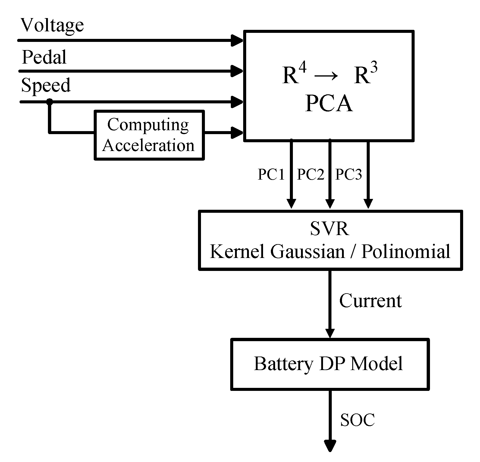
The structure of the current virtual sensor is shown in Figure 1. The battery voltage is obtained by adding the voltage of each one of the 24 battery cells, whose data are available on the CAN bus, rather than using the standard total battery voltage also available on the bus. The acceleration data are obtained by numerical differentiation of the speed measurements. The virtual sensor is formed by two steps. First, a dimension reduction procedure based on PCA is applied to the inputs, and then, the resulting signal is applied to a SVR model that generates the current estimates.

The principal component analysis (PCA) is used to reduce the dimension of input variable space [15]. This methodology allows one to find a new and reduced set of variables (features) as a linear combination of the original variables.

The expression of the principal components (PCs) can be written as:

$$P{C}_i=A{Z}_i$$

(1)

where, considering the i-th sample of input data, $P{C}_i\in {\mathbb{R}}^p$ is the vector of the p principal components, $Z_i\in {\mathbb{R}}^q$ the vector of q input variables and $A\in {\mathbb{R}}^{p\times q}$ the PCA matrix. Each row $a_k$ of matrix A is the eigenvector corresponding to the k-th principal component of the input sample being considered. If we are considering N samples of data, in our case time samples, we can write for all data $PC=AZ$ with $PC\in {\mathbb{R}}^{p\times N}$, and $Z\in {\mathbb{R}}^{q\times N}$. In principle p can be as large as q, but the main idea of PCA is to have $p<q$.

Before being fed to the PCA algorithm, the four input variables (i.e., voltage, pedal, speed and acceleration) are normalized in order to obtain the PCA input data vectors $Z_p$. Each variable is re-scaled as

$$Z_i=\frac{z_i-z_{min}}{z_{max}+z_{min}}$$

(2)

where $z_{max}$ and $z_{min}$ are respectively the maximum and minimum values of the original data samples.

When applied to the data in Table 1, the PCA method finds that three principal components are sufficient to describe, respectively, the $99.75\%,99.78\%,99.58\%$ and $99.66\%$ of the total variance of the input variables for each one of the routes considered. While this means that the feasible order reduction is only one dimension, this reduction, as will be shown in the sequel, allows a substantially better performance of the SVR algorithm.

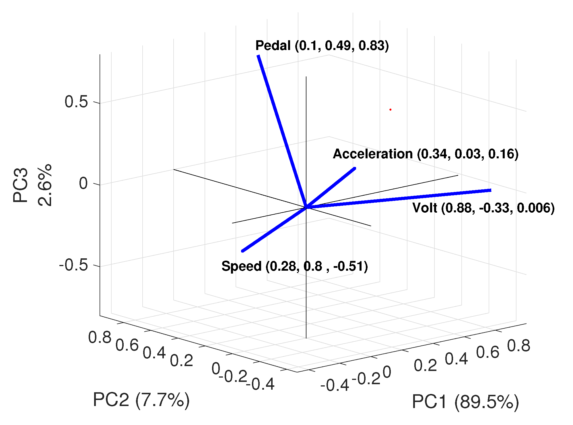
A geometric visualization of the four vectors representing the coefficient values that transform each input variable in the corresponding PC for Route 1 is shown in Figure 2.

The support vector regression (SVR) method was first designed to solve nonlinear two-class classification problems [16,17]. The SVR method is a non-parametric function approximation technique because it relies on kernel functions [18]. The relationship between the independent and dependent variables is represented by a deterministic function, defined as:

$$y=f\left(x\right)=w^T\varphi \left(x\right)+b$$

(3)

where $x\in {\mathbb{R}}^n$ is the independent component of the data and the corresponding dependent value is $y\in \mathbb{R}$, so that each sample vector $x_i$ corresponds to a scalar $y_i$. $w\in {\mathbb{R}}^m$, with m the dimension of the “feature” space, controls the flatness of the model; $\varphi (·)$ is a non-linear mapping function from the input space ${\mathbb{R}}^n$ to feature space ${\mathbb{R}}^m$; and $b\in \mathbb{R}$ is a bias term.

To maximize flatness, a vector w with a small norm is desired; for this reason the coefficients of w are estimated by minimizing:

$$\underset{w,\xi ,{\xi }^{*}}{min}\frac{1}{2}{w}^{T}w+C\sum _i{({\xi }_i+{\xi }_i^{*})}^2$$

(4)

subject to constraints

$$\begin{array}{c}{w}^T\varphi \left(x_i\right)+b-y_i\le \epsilon +{\xi }_i^{*}\\ y_i-w^T\varphi \left(x_i\right)+b\le \epsilon +{\xi }_i\end{array}$$

(5)

where $\epsilon$ is the acceptable output error. C represents a positive constant that determines the degree of penalized loss when a training error larger than $\epsilon$ occurs. ${\xi }_i$ and ${\xi }_i^{*}$ are non negative slack variables specifying the upper and lower “additional” training errors with respect to the allowed error tolerance $\epsilon$.

The optimization dual problem is solved using Lagrangian multipliers, where the optimum is a saddle point of the Lagrangian Equation (6), subject to Equation (7).

$$\begin{array}{cc}\hfill min\frac{1}{2}& \sum _{i,j=0}^N({\alpha }_i-{\alpha }_i^{*})({\alpha }_j-{\alpha }_j^{*})\langle \varphi \left(x_i\right),\varphi \left(x_j\right)\rangle \hfill \\ \hfill & +\epsilon \sum _{i,j=0}^N({\alpha }_j+{\alpha }_j^{*})-\sum _{i,j=0}^N{y}_i({\alpha }_j-{\alpha }_j^{*})\hfill \end{array}$$

(6)

subject to

$$\begin{array}{c}{\sum }_{i=0}^N({\alpha }_i-{\alpha }_i^{*})=0\\ 0\le {\alpha }_i,{\alpha }_i^{*}\le C\\ i=1,2,\dots ,N\end{array}$$

(7)

where N is the number of training samples.

The approximation function $f\left(x\right)$ is defined as:

$$f\left(x\right)=\sum _{i=0}^N({\alpha }_i-{\alpha }_i^{*})G(x_i,x)+b$$

(8)

where ${\alpha }_i$ and ${\alpha }_i^{*}$ are the Lagrange multipliers. The inner product $\langle \varphi \left(x_i\right),\varphi \left(x_j\right)\rangle$ is defined through a kernel function; that is, $G(x_i,x_j)=\langle \varphi \left(x_i\right),\varphi \left(x_j\right)\rangle$ [19,20,21]. Different kernel functions can be employed. In this work we consider the following:

(a) Gaussian kernel (GK):

$$G(x_i,x_j)=-exp\left(\frac{{∥x_i-x_j∥}^2}{2{\sigma }^2}\right)$$

(9)

(b) Polynomial kernel (PKp):

$$G(x_i,x_j)={(c+x_i^T{x}_j)}^p$$

(10)

where ${\sigma }^2$ denotes the variance for GK, p is the order of the kernel and c is a constant that allows one to trade off the influence of the higher and lower order term for PKp. One of the aims of the paper is to show how the choice of the kernel is a key point in the proposed methodology. In the following, the SVR is based on the Gaussian kernel (GK) and the second and sixth order polynomial kernel (PK2 and PK6, respectively).

According to Equation (8), the virtual sensor design problem can now be transformed into the following system of linear equations,

$$\widehat{I}\left(x\right)=\sum _{i=0}^N({\alpha }_i-{\alpha }_i^{*})G(x_k,x_i)+b$$

(11)

where $\widehat{I}\left(x\right)$ is the estimated battery current and $G(·,·)$ is the chosen kernel function; i.e., Gaussian or polynomial kernel.

The k-th input variable sample $x_k$ used for training is set to $x_k=[PC{1}_k,PC{2}_k,PC{3}_k]$ in the PCA case, or to $x_k=[V_k,P_k,S_k,A_k]$, i.e., the scaled voltage ($V_k$), pedal position ($P_k$), vehicle speed ($S_k$) and acceleration ($A_k$), when the SVR model is trained without resorting to PCA.

The performance of the virtual sensor obtained from the SVR procedure, in terms of RMSE (root mean square error) and MAE (mean absolute error), for the GK and PK2 models, wherein PCA was not used, and the PCA + GK, PCA + PK2 and PCA + PK6 models, PCA based, are presented in

Table 2. RMSE (root mean square error) of SVR training for GK, PK2, PCA + GK, PCA + PK2 and PCA + PK6 models.

SVR Training RMSE (A)
Route	GK	PK2	PCA + GK	PCA + PK2	PCA + PK6
1	11.6	46.1	3.58	10.6	4.16
2	29.6	49.0	6.16	14.1	6.73
3	32.9	35.3	10.3	18.2	13.3
4	17.9	123	8.15	17.1	11.2

and

Table 3. Mean absolute error (MAE) of SVR training for GK, PK2, PCA + GK, PCA + PK2 and PCA + PK6 models.

SVR Training MAE
Route	GK	PK2	PCA + GK	PCA + PK2	PCA + PK6
1	2.60	38.2	1.43	4.78	1.91
2	9.50	42.2	2.31	6.54	2.89
3	11.9	29.8	4.10	10.3	6.53
4	6.46	99.1	2.98	7.37	3.50

. In those experiments, different routes have been used for training models, and each model was then tested on the same set used for its training.

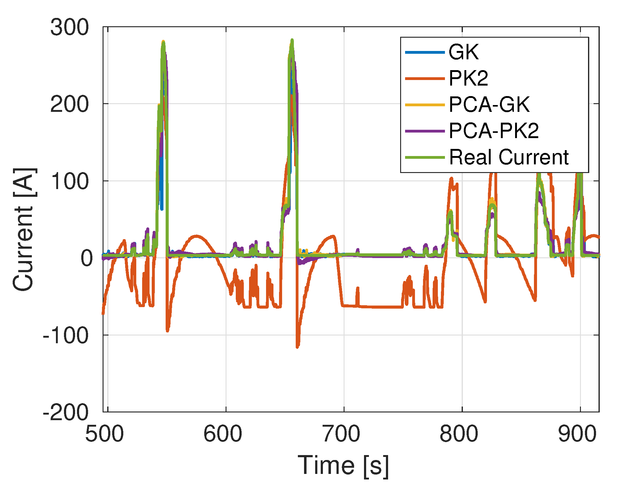
The PCA + GK SVR method offers the best performance on the training sets, with the lowest RMS and MAE values. Additionally, the PCA + PK6 method yields good results, but is in general more expensive in terms of computational requirements. Note also that the route data used for training also has a relevant effect on the final quality of the model. In all cases, note how the use of PCA to pre-process the input variables yields much better results with both the polynomial and the Gaussian kernels. Figure 3 shows the result for each method, except PCA + PK6, over a portion of the training data, in this case extracted from Route 1.

The MAE and RMSE indices in Table 2 and Table 3 only show the average error in model operation and do not give any information about the error distribution. To overcome this problem we propose to use the developed discrepancy ratio (DDR) index, proposed in the literature for evaluating prediction models; see, e.g., [22,23,24,25].

DDR is defined as:

$${DDR}_k=\frac{PredictedValu{e}_k}{MeasuredValu{e}_k}-1$$

(12)

where the optimal result is zero for every sample k.

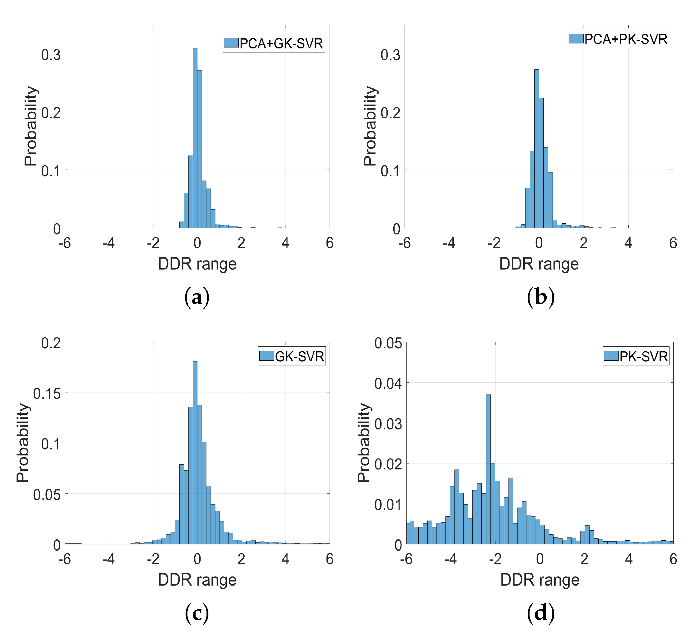
The error distribution can be visually described by drawing the histogram of the DDR for each one of the four different approaches considered. These results (see Figure 4) show that during the training stage, the DDR values for the PCA + GK method vary between −0.9 and 1; those for the PCA + PK2 method between −1 and 2; those for the GK method between −1 and 2; and those for the PK2 model between −5 and 5. Moreover, as it can be seen, the distribution for PCA + GK, and to a lesser degree, for PCA + PK2, has a smaller variance around the optimal zero value, and is thus more reliable than the other methods that do not rely on a preliminary PCA of input variables.

According to the results shown in Table 2 and Table 3, and to the distribution of DDR values shown in Figure 4, only the methods based on PCA “preprocessing” deserve being considered.

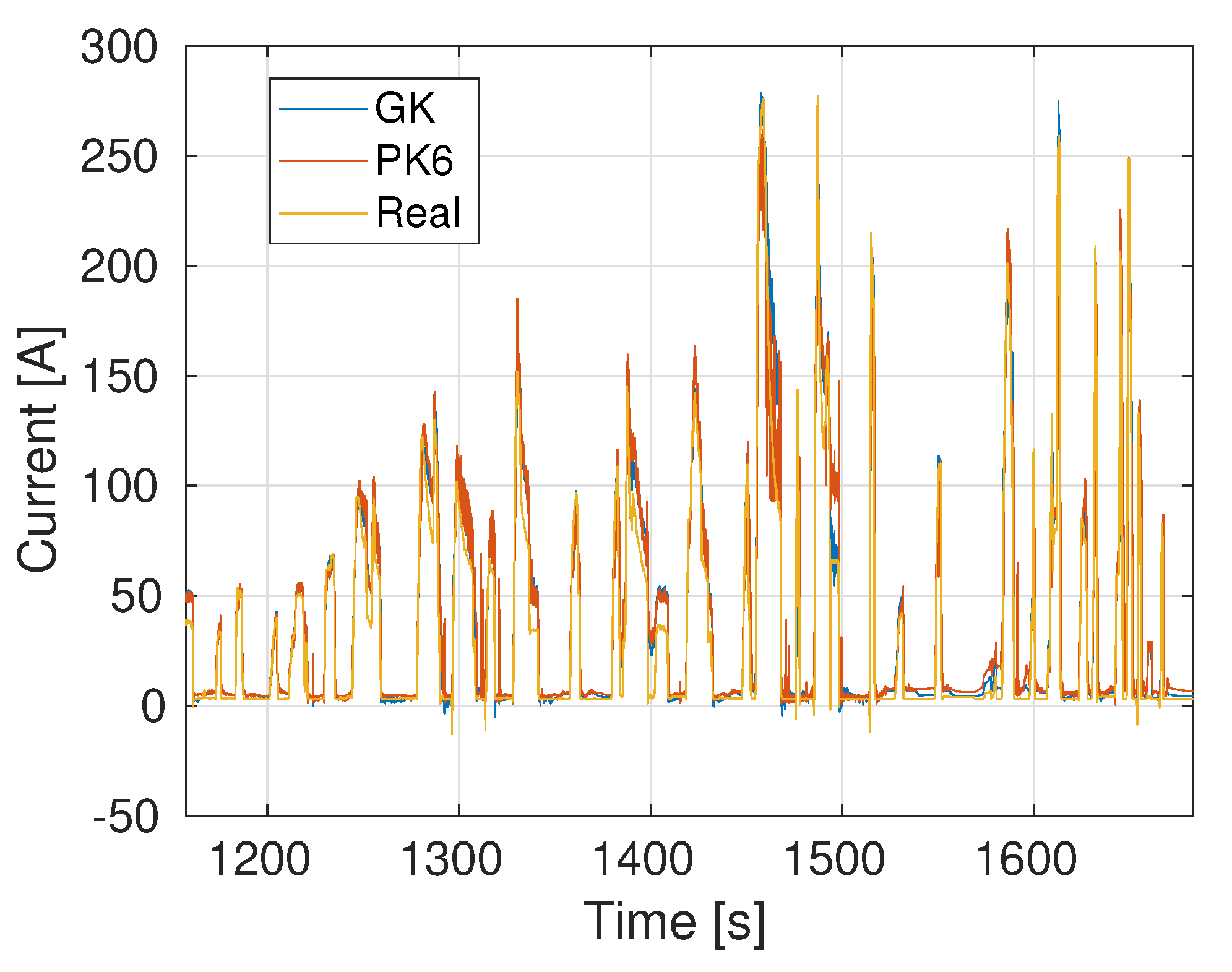
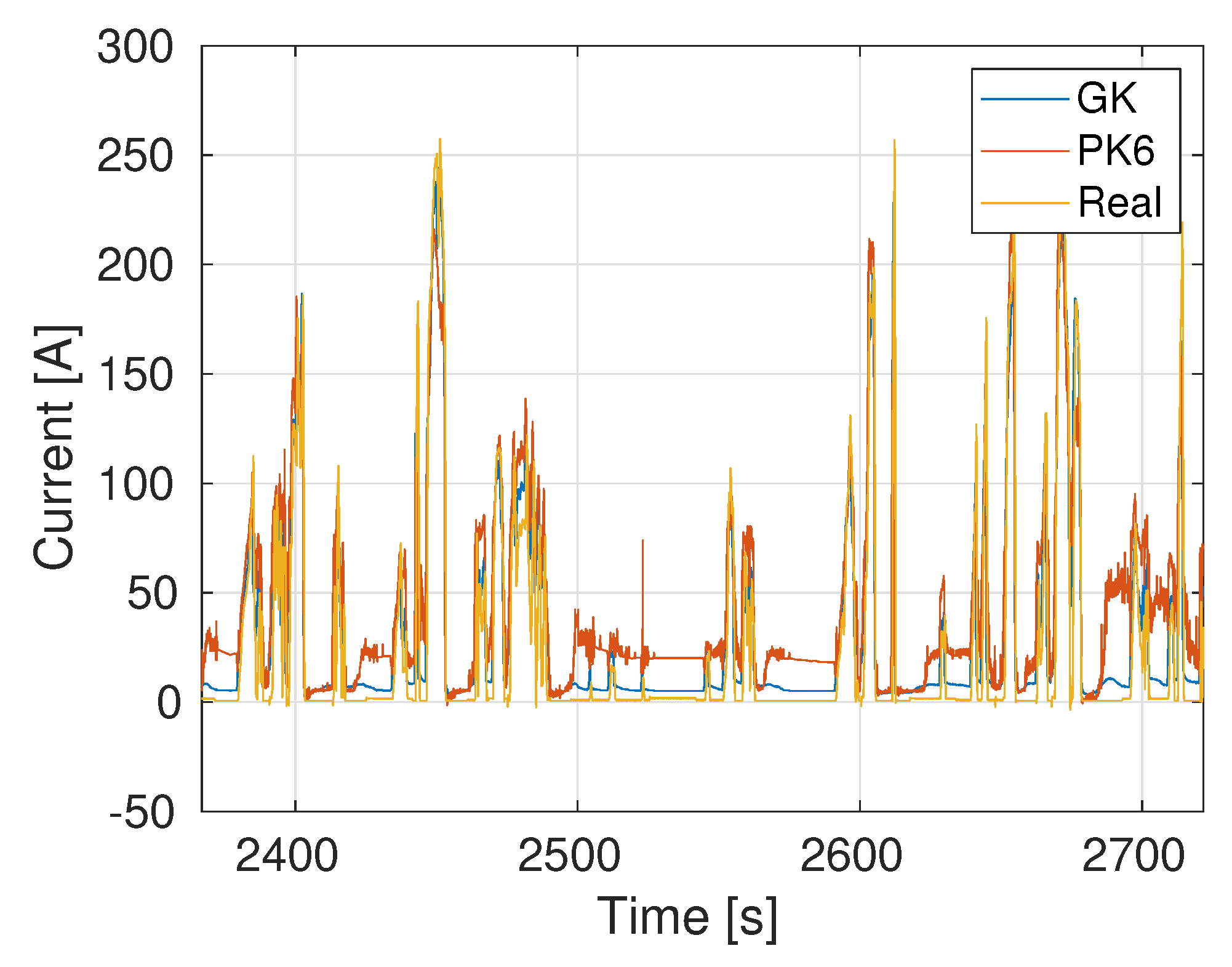
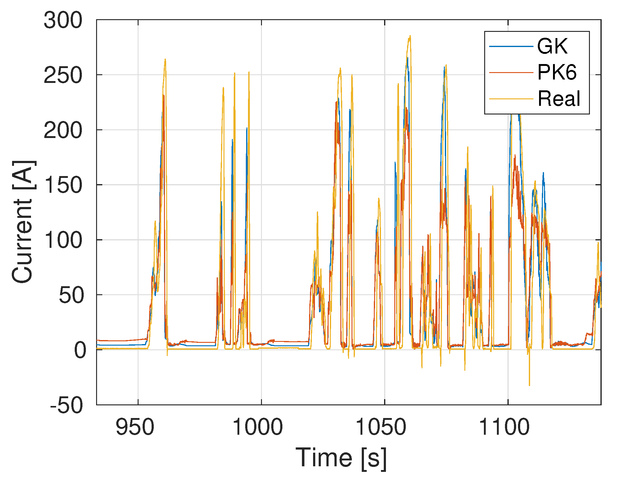
As noted previously, training sets extracted from each one of the four routes considered result in different qualities of virtual sensor. Using, for example, data extracted from Route 1 (900 s) to train the model, the battery current estimations obtained using the data from Routes 2, 3 and 4 are shown, respectively, in Figure 5, Figure 6 and Figure 7. As expected, the Gaussian kernel based model PCA + GK yields the best results, even if the PCA + PK6 model still gives accurate results.

The RMSEs and MAEs of the three models considered, i.e., PCA + GK, PCA + PK2 and PCA + PK6, trained using a 15’ section of each route in the data set, and then tested on the complete data of the four routes, are reported in

Table 4. RMSEs of SVR PCA + GK, PCA + PK2 and PCA + PK6 models trained using four routes tested against the other routes.

Training		Test Route
Model-Route		1	2	3	4	Score
PCA + GK	1	3.98	14.44	14.77	16.91	12.53
	2	9.16	8.03	17.38	19.83	13.6
	3	16.93	19.71	12.21	16.18	16.26
	4	17.04	39.08	13.13	9.26	19.63
PCA + PK2	1	12.75	17.80	19.77	31.84	20.54
	2	19.49	15.30	19.85	18.88	18.38
	3	26.39	29.02	21.07	26.52	25.75
	4	22.26	24.32	21.32	19.43	21.83
PCA + PK6	1	4.99	15.80	14.26	27.33	15.60
	2	11.13	9.55	17.55	12.47	12.68
	3	20.97	20.13	15.01	16.58	18.17
	4	18.36	25.75	16.37	12.33	18.20

and

Table 5. MAEs of SVR PCA + GK, PCA + PK2 and PCA + PK6 models trained using four routes tested against the other routes.

Training		Test Route
Model-Route		1	2	3	4	Score
PCA + GK	1	1.74	6.89	7.17	7.12	5.73
	2	5.21	3.01	10.18	11.22	7.40
	3	8.38	10.01	7.13	7.83	8.34
	4	8.90	13.23	7.75	4.59	8.62
PCA + PK2	1	5.88	17.80	19.77	16.19	14.91
	2	9.22	8.13	11.00	9.99	9.59
	3	13.45	16.01	10.76	12.15	13.09
	4	10.07	13.11	10.13	9.93	10.81
PCA + PK6	1	2.01	7.98	7.15	14.98	8.03
	2	6.84	4.96	8.25	6.64	6.67
	3	11.09	10.33	7.56	8.28	9.32
	4	8.88	14.00	8.22	6.17	9.32

. In each table the column “score” represents the average by row of the RMSE and MAE. Note that the best results were obtained by using the PCA-GK method trained using Route 1 followed by the PCA-PK6 method trained using Route 2. This shows that the characteristics of the routes chosen for the training of the virtual sensors should be carefully chosen to obtain a good representation of the behavior in different situations.

3. Battery Model and SOC Estimation

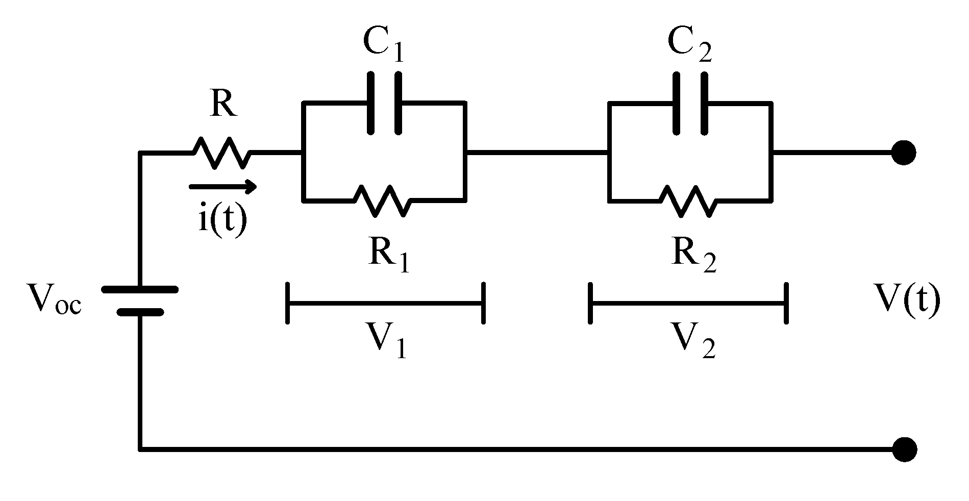
In order to estimate the SOC, the first step is to develop a reliable battery modeling. In this work a model based on the dual polarization (DP) equivalent circuit model is employed to simulate the behavior of the battery cells [10,11]. The DP model is composed of three parts, as shown in Figure 8:

• An ideal voltage source representing the open circuit voltage of the battery $V_{oc}$; this voltage has a non linear relation with the state of charge of the battery. This relation depends on the type of battery, but also on its temperature and age.
• Internal resistors, specifically the “ohmic” resistance represented by R and the polarization resistances $R_1$ and $R_2$.
• Capacitors that, in combination with the polarization resistances, are used to characterize the transient response during the transfer of power, represented by $C_1$ and $C_2$.

Assuming the current through the battery as an independent variable, i.e., the battery model in Figure 8 is connected to an independent current source of value $i\left(t\right)$, modeling battery discharge or charge, the battery terminal voltage can be expressed in terms of the state equation and output relation in Equation (13)

$$\begin{array}{c}\left[\begin{array}{c}\dot{V_1}\\ \dot{V_2}\end{array}\right]=\left[\begin{array}{cc}-\frac{1}{R_1{C}_1}& 0\\ 0& -\frac{1}{R_2{C}_2}\end{array}\right]\left[\begin{array}{c}{V}_1\\ V_2\end{array}\right]+\left[\begin{array}{c}\frac{1}{C_1}\\ \frac{1}{C_2}\end{array}\right]i\left(t\right)\\ V\left(t\right)=V_{oc}+i\left(t\right)R+V_1+V_2\end{array}$$

(13)

where $V_1$ and $V_2$ are the voltages in $C_1$ and $C_2$ respectively; $V\left(t\right)$ is the voltage at the battery terminal; and $i\left(t\right)$ is the current in the battery. The state of the battery is represented by $V_1$ and $V_2$ and by the state of charge $SOC$ that defines the open circuit voltage $V_{oc}$.

The $SOC$ is the ratio of the remaining capacity to the nominal capacity of the battery cell and is obtained from the current $i\left(t\right)$ as:

$$SOC\left(t\right)=SOC\left(t_0\right)-\frac{\eta }{Q}{\int }_{t_0}^{t}i\left(\tau \right)·d\tau$$

(14)

where $i\left(\tau \right)$ is the instantaneous current of the battery, considered as positive for discharge and negative for charge; $\eta$ represents the Coulomb efficiency [26]; and Q is the nominal capacity measured in $Ah$, whose value for the EV used in this work is 150 Ah.

Parameter Estimation

In this section a nonlinear least square (NLS) adaptive algorithm is used to estimate the parameters of the battery. Other methods could be in principle be used, but since in our problem NLS converges quickly and with low computational effort, it has been preferred to alternative methods. In order to minimize the squared error between the measured and calculated voltage, we define as the minimization target function, the error criterion known as chi square, and define it as follows:

$${\chi }^2\left(\psi \right)=\sum _{i=1}^M{\left[\frac{V\left(t_i\right)-\widehat{V}(t_i,\psi )}{{\sigma }_{Vi}}\right]}^2$$

(15)

where $\widehat{V}(\psi ,t)$ is the estimated value of the $V\left(t\right)$ value defined in the output relation of (13) and based on the parameter vector $\psi =\left[R{R}_1{C}_1{R}_2{C}_2{V}_{oc}\right]$; M is the number of data samples used; and ${\sigma }_{Vi}$ is the expected measurement error for the i-th sample $V\left(t_i\right)$.

By collecting all calculated and measured voltages $\widehat{V}\left(t_i\right)$ and $V\left(t_i\right)$ in the $M\times 1$ vectors $\widehat{V}$ and V, respectively, and collecting the reciprocal of all ${\sigma }_{Vi}$ in the $M\times M$ diagonal matrix W, Equation (15) reduces to the quadratic form:

$${\chi }^2\left(\psi \right)={(V-\widehat{V})}^{T}W(V-\widehat{V})$$

(16)

The minimum of the chi square error is searched by repeated use of the Levenberg-Marquardt algorithm, which we briefly recall in the following, on small m sample sized partitions of the M sized available data.

In our setting, the Levenberg-Marquardt algorithm is used to update the parameter vector $\psi$ iteratively by solving the nonlinear optimization problem described in (15). The algorithm adaptively updates the parameter estimates by combining the gradient descent update and the Gauss-Newton update [27] by tuning a damping parameter $\lambda$. The Marquardt’s update equation is given by:

$$[J^{T}WJ+\lambda \mathrm{diag}\left(J^{T}WJ\right)]h=J^{T}W(V-\widehat{V})$$

(17)

where h is the parameter update vector; $\mathrm{diag}(·)$ is an operator that extracts the diagonal from a matrix; J is the Jacobian matrix of $V-\widehat{V}$ with respect to $\psi$; and $\lambda$ is the damping parameter acting on the diagonal of $J^{T}WJ$, and was initially chosen to be large, so that initially, small steps in the steepest descent direction would be taken. The Jacobian can be quickly updated using the Broyden formula [28].

$$J_{new}=J+\frac{(\widehat{V}(\psi +h)-\widehat{V}\left(\psi \right)-Jh)h^T}{\left(h^{T}h\right)}$$

(18)

The damping factor $\lambda$ is adjusted by checking the values obtained with the new parameter set against the previous values. One possible way to do this is by using a $\rho$ factor [27,29,30] defined in (19).

The step is accepted if $\rho$ is larger than a user-specified threshold and rejected otherwise; in this case, $\lambda$ is increased.

$$\rho \left(h\right)=\frac{{\chi }^2\left(\psi \right)-{\chi }^2(\psi +h)}{h^T(\lambda \mathrm{d}iag\left(J^{T}WJ\right)h+J^{T}W(V-\widehat{V}\left(\psi \right))})$$

(19)

Different convergence criteria may be used based on limit values for the gradient, for the chi square error or for the norm of the update vector; or simply, by the number of iterations.

An adaptive algorithm was developed based on the above criterion. Given M time samples of current and voltage data $i\left(t\right)$ and $V\left(t\right)$, the sequence was initially split in sub-sequences of length m. The algorithm optimizes, for each sub-sequence, the ${\chi }^2$ cost function (16), obtained by estimating the electric parameter vector $\psi$ of the battery and then calculating the voltage from the electrical parameters in $\psi$. The operation is repeated for each following sub-sequence using as the initial condition for $\psi$, the values obtained in the previous iteration. This process updates and adjusts the electrical parameters of the battery.

The identification results of electric parameters for the DP battery model are shown in

Table 6. Battery parameters’ estimation.

Identified Item	Value
R	0.0056 $\Omega$
R1	0.040858 $\Omega$
R2	0.025259 $\Omega$
C1	9484 F
C2	71.049 F

.

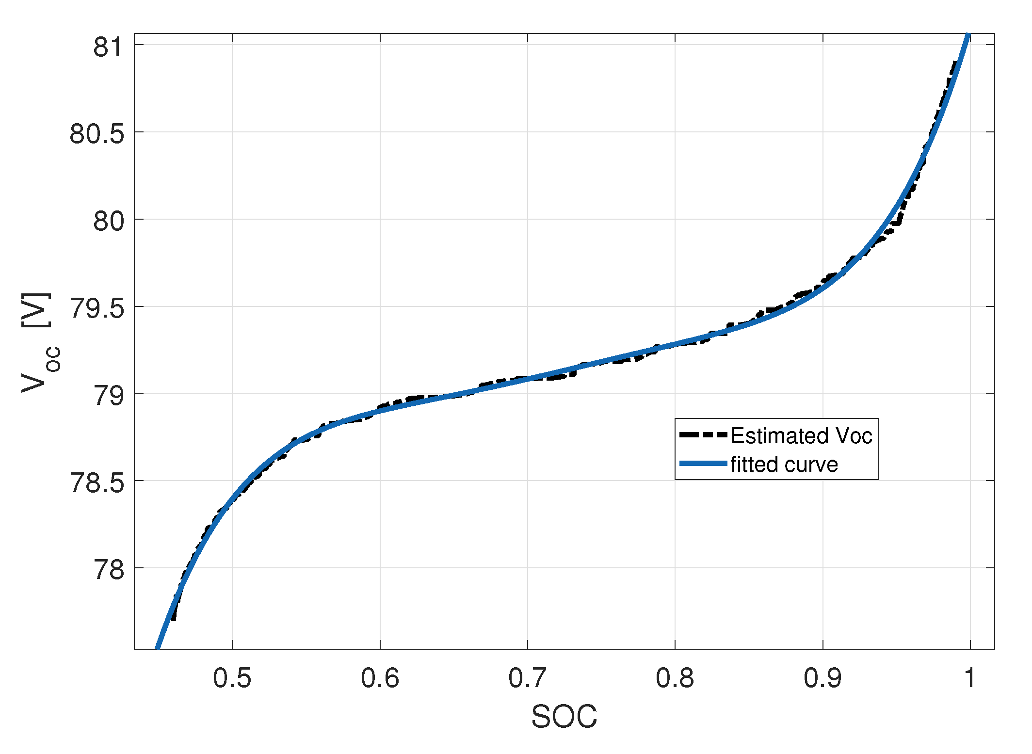
Finally, the relation between $SOC$ and $V_{oc}$ is determined. The relationship between the $V_{oc}$ and the SOC can be described through polynomial data fitting. The fitted curve for the relationship between $V_{oc}$ and SOC is shown in Figure 9, where the $V_{oc}$ from the estimated data is fitted to the SOC value using the $4th$ order regression polynomial in (20).

$$\begin{array}{cc}\hfill V_{oc}\left(SOC\right)& =-157.9SO{C}^4+554.3SO{C}^3-696SO{C}^2+\hfill \\ \hfill & 378.3SOC+4.81\hfill \end{array}$$

(20)

4. Analysis Of Results and Discussion

In this section, the performance of the SOC estimation using the current virtual sensor based on the PCA + GK and PCA + PK2 methods and the DP battery model is evaluated.

The voltage, the pedal position, the speed and the acceleration were measured and were used as input data to the model. PCA was applied, reducing the dimension of the inputs from $R^4$ to $R^3$. Then, the data were injected to the SVR model to estimate the current. Finally, the current provided by the virtual sensor was used as input for the DP battery model, to finally determine the SOC.

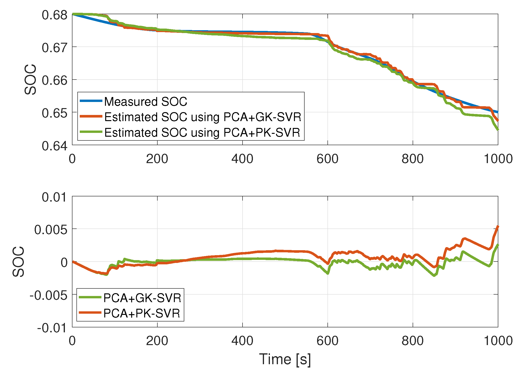
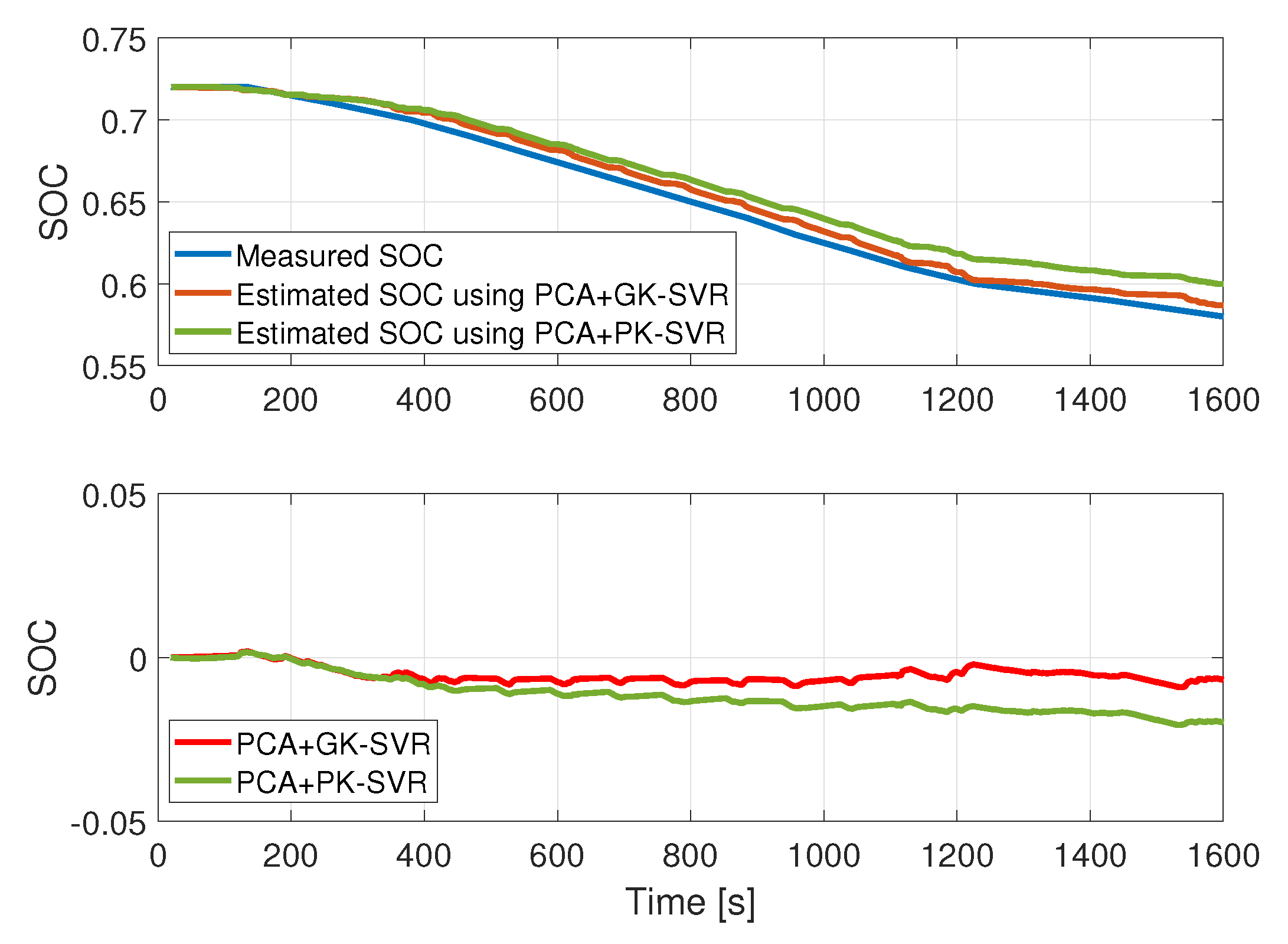
The estimation methods were validated with two routes, and the results can be seen in Figure 10 and Figure 11, where the performance of the estimation methods vs. data reported by the existing BMS is shown.

The FIT index was used to evaluate the quality of the proposed SOC estimation algorithm. This index is defined as

$$FIT=100\left(1-\frac{∥SO{C}_m-SO{C}_e∥}{∥SO{C}_m-\overline{SO{C}_m}∥}\right)\%$$

(21)

where $∥*∥$ is the euclidean norm of the argument, $SO{C}_e$ is the SOC obtained with the proposed estimation method, $SO{C}_m$ the measurement provided by the BMS and $\overline{SO{C}_m}$ is the average of $SO{C}_m$ during the experiment.

Table 7. SOC estimation results for Route 1.

	PCA + GK-SVR	PCA + PK2-SVR
FIT	91.80%	85.423%
RMSE	0.007	0.014
MAE	0.005	0.011

shows a comparison of the methods according to the FIT, RMSE and MAE indices for Route 1. The obtained indices make it clear that the estimation using the PCA + GK method shows higher prediction performance than the PCA + PK2 model, with $FIT=91.8\%$.

For Route 2, results are shown in

Table 8. SOC estimation results for Route 2.

	PCA + GK-SVR	PCA + PK2-SVR
FIT	87.49%	71.76%
RMSE	0.058	0.127
MAE	0.053	0.114

. Once more, the PCA + GK model shows better performance than the PCA + PK2 model, with $FIT=87.49\%$.

Note that both models, PCA + GK and PCA + PK2, provide adequate virtual current measurements that allow the estimation of the battery SOC from the battery voltage, accelerator pedal position and vehicle speed.

5. Conclusions

We have presented a solution for state of charge estimation in electric vehicle applications. The proposed strategy makes use of virtual sensors for the battery current estimation, replacing the physical sensor in case of failure. The models are derived from experimental data captured from the CAN bus of an actual electric vehicle and use the battery voltage, vehicle speed and acceleration pedal position to recover the current signal if the actual measurement is not available.

Support vector regressions and principal component analysis have been employed to build the virtual sensors. Gaussian and polynomial functions have been employed as kernel functions, and it was observed that the Gaussian kernel offers better performance on the available data sets. A principal component analysis allows one to reduce by one the dimension of the input to the virtual sensor, significantly increasing the final performance.

The estimated current signal is used as input to a dual polarization equivalent circuit model of the battery to estimate the state of charge and open circuit voltage during the vehicle’s operation. The parameters of the equivalent circuit have been obtained through a non-linear least squares adaptive algorithm, using experimental data from the vehicle.

The joint operation of the virtual sensor and the battery model allows one to estimate the state of charge with a fit higher than $87\%$ when evaluated on fresh data not employed for the model adjustment.

The methods herein proposed are scalable and can integrate knowledge from other sensors, such as temperature and torque, and can be combined with other machine learning methodologies.

One of the limitations that we noticed in the the method is related to specific properties of the driving segments. Analyzing the entire route can lead to incorrect patterns due to different links between the magnitudes considered by the virtual sensor. For example, accelerations and currents have a very different relation if the vehicle is traveling uphill or on flat terrain, or even downhill. The next extension of our work is to create a mixed method of classification and machine learning, to recognize specific peculiarities of the driving segment and select the correct model to apply.

References

- Tannahill, V.R.; Sutanto, D.; Muttaqi, K.M.; Masrur, M.A. Future vision for reduction of range anxiety by using an improved state of charge estimation algorithm for electric vehicle batteries implemented with low-cost microcontrollers. IET Electr. Syst. Transp. 2015, 5, 24–32. [Google Scholar] [CrossRef]
- Sautermeister, S.; Falk, M.; Bäker, B.; Gauterin, F.; Vaillant, M. Influence of Measurement and Prediction Uncertainties on Range Estimation for Electric Vehicles. IEEE Trans. Intell. Transp. Syst. 2018, 19, 2615–2626. [Google Scholar] [CrossRef]
- Scheubner, S.; Thorgeirsson, A.T.; Vaillant, M.; Gauterin, F. A Stochastic Range Estimation Algorithm for Electric Vehicles Using Traffic Phase Classification. IEEE Trans. Veh. Technol. 2019, 68, 6414–6428. [Google Scholar] [CrossRef]
- Kontou, E.; Yin, Y.; Lin, Z. Socially optimal electric driving range of plug-in hybrid electric vehicles. Transp. Res. Part D Transp. Environ. 2015, 39, 114–125. [Google Scholar] [CrossRef] [Green Version]
- Srinivasa Raghavan, S.; Tal, G. Influence of User Preferences on the Revealed Utility Factor of Plug-In Hybrid Electric Vehicles. World Electr. Veh. J. 2019, 11, 6. [Google Scholar] [CrossRef] [Green Version]
- Hannan, M.A.; Hoque, M.M.; Hussain, A.; Yusof, Y.; Ker, P.J. State-of-the-Art and Energy Management System of Lithium-Ion Batteries in Electric Vehicle Applications: Issues and Recommendations. IEEE Access 2018, 6, 19362–19378. [Google Scholar] [CrossRef]
- Xiong, R.; Cao, J.; Yu, Q.; He, H.; Sun, F. Critical Review on the Battery State of Charge Estimation Methods for Electric Vehicles. IEEE Access 2018, 6, 1832–1843. [Google Scholar] [CrossRef]
- Fotouhi, A.; Auger, D.J.; Propp, K.; Longo, S.; Wild, M. A review on electric vehicle battery modelling: From Lithium-ion toward Lithium–Sulphur. Renew. Sustain. Energy Rev. 2016, 56, 1008–1021. [Google Scholar] [CrossRef] [Green Version]
- Liu, Z.; He, H. Model-based Sensor Fault Diagnosis of a Lithium-ion Battery in Electric Vehicles. Energies 2015, 8, 6509–6527. [Google Scholar] [CrossRef]
- Barcellona, S.; Ciccarelli, F.; Iannuzzi, D.; Piegari, L. Modeling and Parameter Identification of Lithium-Ion Capacitor Modules. IEEE Trans. Sustain. Energy 2014, 5, 785–794. [Google Scholar] [CrossRef]
- Hongwen, H.; Xiong, R.; Jinxin, F. Evaluation of Lithium-Ion Battery Equivalent Circuit Models for State of Charge Estimation by an Experimental Approach. Energies 2011, 4, 582–598. [Google Scholar] [CrossRef]
- Li, Z.; Jiang, S.; Dong, J.; Wang, S.; Ming, Z.; Li, L. Battery capacity design for electric vehicles considering the diversity of daily vehicles miles traveled. Transp. Res. Part C Emerg. Technol. 2016, 72, 272–282. [Google Scholar] [CrossRef] [Green Version]
- Bascetta, L.; Gruosso, G.; Gajani, G. Analysis of Electrical Vehicle behavior from real world data: A V2I Architecture. In Proceedings of the 2018 International Conference of Electrical and Electronic Technologies for Automotive, AUTOMOTIVE 2018, Milan, Italy, 9–11 July 2018. [Google Scholar] [CrossRef]
- Storti Gajani, G.; Gruosso, G.; Valladolid, J.D. Electric Vehicle speed, pedal, accel, voltage and current data over four different roads. IEEE Dataport 2019. [Google Scholar] [CrossRef]
- Archanah, T.; Deshmukh, S. Dimensionality Reduction and Classification through PCA and LDA. Int. J. Comput. Appl. 2015, 122, 4–8. [Google Scholar] [CrossRef]
- Vapnik, V.N. Statistical Learning Theory; Wiley-Interscience: Hoboken, NJ, USA, 1998. [Google Scholar]
- Salcedo-Sanz, S.; Rojo-Álvarez, J.L.; Martinez-Ramon, M.; Camps-Valls, G. Support vector machines in engineering: An overview. Wiley Interdiscip. Rev. Data Min. Knowl. Discov. 2014, 4. [Google Scholar] [CrossRef]
- Drucker, H.; Burges, C.J.C.; Kaufman, L.; Smola, A.J.; Vapnik, V. Support Vector Regression Machines. In Advances in Neural Information Processing Systems 9; Mozer, M.C., Jordan, M.I., Petsche, T., Eds.; MIT Press: Cambridge, MA, USA, 1997; pp. 155–161. [Google Scholar]
- Schölkopf, B.; Smola, A. Learning with Kernels: Support Vector Machines, Regularization, Optimization, and Beyond; Adaptive Computation and Machine Learning, Parts of this book, including an introduction to kernel methods, can be downloaded; MIT Press: Cambridge, MA, USA, 2002; p. 644. [Google Scholar]
- Ding, Y.; Cheng, L.; Pedrycz, W.; Hao, K. Global Nonlinear Kernel Prediction for Large Data Set With a Particle Swarm-Optimized Interval Support Vector Regression. IEEE Trans. Neural Netw. Learn. Syst. 2015, 26, 2521–2534. [Google Scholar] [CrossRef] [Green Version]
- Rojo-Álvarez, J.L.; Martínez-Ramón, M.; Muñoz-Marí, J.; Camps-Valls, G. Advances in Kernel Regression and Function Approximation. In Digital Signal Processing with Kernel Methods; John Wiley and Sons, Ltd.: Hoboken, NJ, USA, 2018; Chapter 8; pp. 333–385. Available online: http://xxx.lanl.gov/abs/https://onlinelibrary.wiley.com/doi/pdf/10.1002/9781118705810.ch8 (accessed on 4 February 2020).
- Noori, R.; Khakpour, A.; Omidvar, B.; Farokhnia, A. Comparison of ANN and principal component analysis-multivariate linear regression models for predicting the river flow based on developed discrepancy ratio statistic. Expert Syst. Appl. 2010, 37, 5856–5862. [Google Scholar] [CrossRef]
- Haghiabi, A.H.; Parsaie, A.; Ememgholizadeh, S. Prediction of discharge coefficient of triangular labyrinth weirs using Adaptive Neuro Fuzzy Inference System. Alex. Eng. J. 2018, 57, 1773–1782. [Google Scholar] [CrossRef]
- Hooshyaripor, F.; Tahershamsi, A.; Behzadian, K. Estimation of peak outflow in dam failure using neural network approach under uncertainty analysis. Water Resour. 2015, 42, 721–734. [Google Scholar] [CrossRef] [Green Version]
- Huang, Y.; Clerckx, B. Relaying Strategies for Wireless-Powered MIMO Relay Networks. IEEE Trans. Wirel. Commun. 2016. [Google Scholar] [CrossRef] [Green Version]
- Sidhu, A.; Izadian, A.; Anwar, S. Adaptive Nonlinear Model-Based Fault Diagnosis of Li-Ion Batteries. IEEE Trans. Ind. Electron. 2015, 62, 1002–1011. [Google Scholar] [CrossRef] [Green Version]
- Bellavia, S.; Gratton, S.; Riccietti, E. A Levenberg–Marquardt method for large nonlinear least-squares problems with dynamic accuracy in functions and gradients. Numerische Mathematik 2018. [Google Scholar] [CrossRef] [Green Version]
- Mohammad, H.; Waziri, M.Y. On Broyden-like update via some quadratures for solving nonlinear systems of equations. Turk. J. Math. 2015, 39, 335–345. [Google Scholar] [CrossRef]
- Transtrum, M.K.; Sethna, J.P. Improvements to the Levenberg-Marquardt algorithm for nonlinear least-squares minimization. arXiv 2012, arXiv:physics.data-an/1201.5885. [Google Scholar]
- Qiao, J.; Wang, L.; Yang, C.; Gu, K. Adaptive Levenberg-Marquardt Algorithm Based Echo State Network for Chaotic Time Series Prediction. IEEE Access 2018, 6, 10720–10732. [Google Scholar] [CrossRef]
Figure 1.
General description of the architecture used for state of charge estimation (SOC) estimation.
Figure 2.
Input variable vector representation in the principal components’ space.
Figure 3.
A sample of predicted current on the same route used for training—in this case Route 1. The PCA + PK6 model is not shown.
Figure 4.
Normalized histogram of the developed discrepancy ratio (DDR) values for the four methods in the training stage. (a) PCA + GK-SVM, (b) PCA + PK2-SVM, (c) GK-SVM and (d) PK2-SVM.
Figure 5.
Current prediction: Training using a 15’ sample of Route 1 and Testing on a small portion of Route 2.
Figure 6.
Current prediction: Training using a 15’ sample of Route 1 and Testing on a small portion of Route 3.
Figure 7.
Current prediction: Training using a 15’ sample of Route 1 and Testing on a small portion of Route 4.
Figure 8.
Thevenin battery model (2RC model).
Figure 9.
Estimated and fitted vs. SOC (DP model).
Figure 10.
SOC model for Route 1. Top panel: SOC value; bottom panel: Error.
Figure 11.
SOC model for Route 2. Top panel: SOC value; bottom panel: Error.