On the Introduction of Canny Operator in an Advanced Imaging Algorithm for Real-Time Detection of Hyperbolas in Ground-Penetrating Radar Data

Abstract

This paper focuses on the use of the Canny edge detector as the first step of an advanced imaging algorithm for automated detection of hyperbolic reflections in ground-penetrating radar (GPR) data. Since the imaging algorithm aims to work in real time; particular attention is paid to its computational efficiency. Various alternative criteria are designed and examined, to fasten the procedure by eliminating unnecessary edge pixels from Canny-processed data, before such data go through the subsequent steps of the detection algorithm. The effectiveness and reliability of the proposed methodology are tested on a wide set of synthetic and experimental radargrams with promising results. The finite-difference time-domain simulator gprMax is used to generate synthetic radargrams for the tests, while the real radargrams come from GPR surveys carried out by the authors in urban areas. The imaging algorithm is implemented in MATLAB.

1. Introduction

Ground-penetrating radar (GPR) is the most effective and mature non-destructive inspection method for the detection of underground objects and for the high-resolution imaging of soil structures [1]. Among its numerous applications in different fields, GPR enables the localization (position, depth) and characterization (size, material) of hidden utilities, even when the signal-to-noise ratio is quite low [2,3,4]. Utilities made of different materials can be found using a GPR, including metal, plastic, concrete, and asbestos; other underground features can be mapped, too, such as cavities, basements, foundations, concrete layers, and more. GPR detection of utilities has important limitations, too. In particular, a GPR signal cannot always be unambiguously associated with a specific kind of utility and an accurate estimation of the target size is not straightforward. Moreover, the penetration of GPR signals in the soil is limited by electromagnetic emission restrictions established by law, in addition to being strongly dependent on the frequency band of the employed antennas and environmental conditions, which implies that sometimes deep services cannot be found. The minimum size of detectable targets and the minimum distance between distinguishable targets depend on the resolution of the GPR, which is related to the gain and frequency band of the used antennas. In the presence of many scattered fragments (such as stones and debris), tree roots, or other disturbing targets, it may be very difficult to distinguish the responses of the sought utilities.

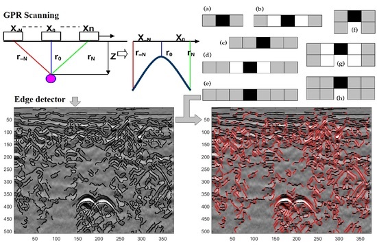
According to a nomenclature widely accepted by the GPR community, the term ‘A-scan’ refers to an array of electric-field amplitude values measured by the GPR in a fixed position and in N consecutive instants [5]. The term ‘B-scan’, instead, corresponds to a matrix of electric-field amplitude values measured by the GPR in N time instants and in M different positions, meaning a set of M A-scans (the B-scan is also called ‘radargram’ or ‘profile’). In the common-offset method, which is the data acquisition strategy used most often, a B-scan is recorded by moving a GPR along a line, e.g., parallel to the air-soil interface, and by recording M A-scans in equally spaced positions.

The presence of a circular-section cylindrical target in the subsurface, with axis orthogonal to the acquisition line, generates a hyperbolic signature in a B-scan [1,6]. From the coordinates of the hyperbola vertex and from the slope of its asymptotes, the position and size of the target can be estimated [5,7]. From the slope of the asymptotes it is also possible to infer the relative permittivity of the material hosting the target [1]. Smaller targets produce smaller hyperbolas, larger targets produce larger hyperbolas; if the GPR acquisition line crosses a target orthogonal to its axis, the hyperbola is narrower than it would be if the GPR were moved along a line forming an angle smaller than 90° with the target axis. A fixed target, buried in the same material at different depths, yields different hyperbolas: the shallower the target is, the narrower the hyperbola, while hyperbolas are broader for deeper targets. A fixed target buried at a given depth but in different materials, produces different hyperbolas, too: in a high-permittivity material (e.g., wet clay), the hyperbolas are narrower than in materials with a lower permittivity (e.g., dry sand).

The most commonly used approaches to identify and classify hyperbolic signatures in radargrams are manual, which is time-consuming [8,9,10]. In particular, most software tools for the processing of GPR data, such as GPRslice [11], Reflexw [12], and matGPR [13], allow the hyperbolic signatures visible in radargrams to be analyzed in an immediate graphical way. Typically, the user can superimpose on each hyperbolic signature a modeled hyperbola; the parameters involved in the fitting process are the propagation velocity of electromagnetic waves in the medium hosting the target, the radius of the target, and the coordinates of its centre (depth and location along the scan line); such parameters can be changed interactively and thus the properties of the modeled hyperbola can be varied, until the superposition looks accurate enough. The quality of fitting is determined by the eye and depends on the experience of the user. The hyperbola fitting method is based on the assumption on non-dispersive propagation in a uniform half-space and provides accurate results when dealing with point diffractors or small circular-section targets.

The development of efficient, robust, and accurate algorithms capable of automatically finding hyperbolas in radargrams is currently a subject of high interest in the GPR scientific community [14], especially for real-field applications. To this aim, various supervised and unsupervised procedures have been proposed in the scientific literature; they make use of: Hough transform [15,16,17], radon transformation [18], wavelet transform [19], the Viola-Jones learning algorithm [20], or standard algorithms for pattern recognition, such as support vector machines [21,22,23] and artificial neural networks [24,25,26]. A novel method for the detection and localization of target signatures in radargrams, denominated SPOT-GPR (sub-array processing open tool for GPR applications), implements a sub-array processing method based on the use of smart-antenna and radar techniques [27,28,29]. Another interesting approach is proposed and tested in [30]: the apices of well- and ill-shaped hyperbolas are automatically detected in radargrams by fitting an analytical function of a hyperbola to the profile edge dots detected with the Canny filter. The recently-proposed algorithm APEX (automated point extraction from radargrams) [14] is capable of finding the coordinates of hyperbola apices and extract the points on hyperbola prongs; it is based on the use of a cascade object detector (COD) to identify segments of interest that contain hyperbolic reflections and on a simple but smart procedure for the local search of apices. APEX has been successfully tested on synthetic data and experimental data recorded in complex urban environments during real GPR utility surveys [31,32,33]. A comparative analysis of APEX and SPOT-GPR is presented in [34].

While the goal of various quantitative microwave imaging techniques for GPR applications (including APEX and SPOT-GPR) is to detect, localize and characterize discrete buried objects, other approaches aim at an overall electromagnetic reconstruction of the underground structures, and more specifically at a qualitative or quantitative estimation of the geometrical distribution of the physical properties of media (dielectric permittivity, electric conductivity) in the subsurface [35,36]. Such methods are promising for the analysis of radargrams obtained in highly heterogeneous environments [37]. Sparse reconstruction algorithms find application in the imaging of targets embedded in stratified dielectric media [38,39]. Moreover, fast and accurate forward solvers [40,41,42,43,44] are of high interest in this area of research, too, because they can be combined with imaging algorithms and full-wave inversion techniques [45,46].

In this complex and variegated framework of microwave imaging techniques for GPR applications, the present paper investigates the possibility to upgrade the aforementioned APEX algorithm by introducing the Canny edge detector in its first stage. The primary motivation for this upgrade was to make the algorithm faster and suitable to be employed in real-time applications, however the upgrade has turned out to be useful for improving the robustness and effectiveness of the algorithm, too.

As is known, an edge can be defined as a set of connected pixels lying on the border line between two different regions [47]. Edge detection is the forefront of image processing for object detection and is crucial for computer vision: in fact, various algorithms have been developed through the decades to detect edges in images.

Roberts Cross operator, initially proposed by Lawrence Roberts in 1963, was one of the first edge detectors [48]; this algorithm performs a simple gradient measurement on the image, namely it approximates the image gradient through discrete differentiation which is achieved by calculating the sum of the squares of the differences between diagonally adjacent pixels. In this way, Roberts Cross operator highlights regions of high spatial frequency, which often correspond to edges. The main reasons for using Roberts Cross operator are its computational speed and the absence of parameters to set; the main disadvantage is that the algorithm is very sensitive to noise and produces weak responses to genuine edges unless they are very sharp.

Sobel operator [49] is based on convolving the image with a small, separable, and integer valued filter in both the horizontal and vertical directions; it is slower to compute than Robert Cross, but has the advantage of simultaneously providing differentiation (which gives the edge response) and gaussian smoothing (which reduces noise), so it is less sensitive to noise and normally produces considerably higher output values for similar edges, compared with Roberts Cross.

Prewitt gradient edge detector [50] works in a very similar way to Sobel but uses slightly different kernels: it produces similar results but is less isotropic in its response.

Laplacian operator [51] is somewhat different from the filters mentioned so far and computationally faster; it uses only one kernel and it calculates second order derivatives in a single pass. It sometimes produces exceptional results but is very sensitive to noise and to correct this issue images are often Gaussian smoothed before applying Laplacian filter.

Canny operator [52] was proposed by John F. Canny in 1986 and is the most commonly used edge detection method. It is more complex than the algorithms mentioned above and works in a multi-stage process. First, the image is Gaussian smoothed. Then, a first derivative operator based on Roberts Cross is applied to highlight image regions with high first spatial derivatives; here, edges cause the presence of ridges in the gradient magnitude image. Canny algorithm tracks the top of these ridges and sets to zero all pixels that are not on the ridge top, to provide a thin line in the output image (this step of the algorithm is called non-maximal suppression). The tracking process exhibits hysteresis controlled by two thresholds, where tracking can only begin at a point on a ridge higher than the lowest threshold and continues in both directions out from that point until the height of the ridge falls below the highest threshold (hysteresis is useful to ensure that noisy edges are not broken up into multiple edge fragments). Canny operator is computationally more expensive compared to Roberts Cross, Prewitt, Sobel, and Laplacian; however, it performs better than all those operators and many others under almost all scenarios and it is widely recognized as the most effective edge-detection method [53,54,55]. For these reasons, and because of the successful application of Canny operator to GPR data shown in [30], Canny operator has been identified as the most favorable edge-detection algorithm to be embedded into APEX.

As far as the methodology presented in this paper is concerned, when embedding Canny edge operator into APEX, special attention has been paid to optimizing the time needed by the edge detector to operate on the entire radargram. Moreover, it has been observed that Canny-processed radargrams still contain many unwanted edge pixels, which are not useful for the purposes of finding and analyzing hyperbolas. Therefore, suitable test conditions have been conceived and tested, to delete unnecessary edge pixels from Canny-processed radargrams before they are passed to the next steps of the hyperbola detection algorithm. Canny edge operator and the proposed test conditions have been applied to a wide set of experimental and synthetic data: experimental data were recorded over different urban scenarios, with various radar settings; synthetic data were calculated by using the finite-difference time-domain simulator gprMax [40,56], sometimes with the aid of an in-house computer-aided design tool [40,57]. Promising results have been obtained.

In Section 2, materials and methods are presented: the basic principles of APEX (Section 2.1) and Canny edge operator (Section 2.2) are resumed; the introduction of Canny operator into APEX is explained (Section 2.3); and, the synthetic and experimental datasets used to test the proposed procedure are presented (Section 2.4). In Section 3, the results obtained are reported and discussed. The paper is concluded with Section 4, where final remarks are given and future work is envisaged.

2. Materials and Methods

2.1. Automated Point Extraction from Radargrams (APEX) Algorithm

APEX (automated point extraction from radargrams) was recently developed with the primary objective of automatically detecting hyperbolic signatures in radargrams [14,31,32,33].

Only small portions of a radargram usually contain objects of interest. Therefore, in the first stage of the algorithm, APEX uses a trained COD [58] to pick out of a radargram the regions that might contain objects of interest; such regions are denominated segments of interest (SOIs) (see Figure 1). The COD is trained on a dataset containing positive and negative samples, where positive samples are hyperbolic reflections and negative samples are different signatures (for example, reflections by soil layers and non-cylindrical objects). Then, APEX carries out a coarse analysis of the SOIs and deletes the redundant segments (i.e., SOIs corresponding to regions already included in other SOIs). The remaining SOIs are sent to the next stage of the algorithm.

Now APEX carries out a pixel analysis of each SOI, which aims at finding the coordinates of the apices of all hyperbolas and at identifying all pixels lying on hyperbola prongs.

For the hyperbola apex search, each SOI is divided column-wise into three equal parts. In the pixel column at the edge between the first and second part, the pixel with highest intensity is found. This pixel becomes the starting point for the apex search. The subsequent search is not limited to the selected SOI but is conducted on the entire radargram. Assuming that the sought apex is on the right side with respect to the starting pixel, a first search goes in that direction. A 3 × 2 submatrix is created, with the starting pixel in the second row and first column. The local maximum is found within the other five pixels. Such a local maximum becomes the new starting pixel and a new 3 × 2 submatrix is created, with this new starting pixel in the second row and first column. The local maximum is again found within the other five pixels; and the procedure continues until the apex is found. The submatrix is expected to move up and right; when it moves downwards, this probably means that the apex was already found, hence a constraint is checked to eventually cancel a further search. In particular, each time the submatrix remains in the same row or moves down, a parameter denominated “sum of moves” is increased by 1, or else it is set to zero. This parameter is used to constrain further searches: when the “sum of moves” exceeds a threshold, the search is stopped. The threshold does not have the same value for every radargram, and it mostly depends on the number of samples per scan: the bigger the number of samples per scan, the higher the value of the threshold [14]. It is possible that a SOI includes the right prong of hyperbolic reflection as well; thus, a second search is carried out where the starting pixel is between the second and third part of the SOI, instead of being between the first and second parts, and the search is conducted in the left segment of the radargram, with the starting pixel in the second row and second column of a 3 × 2 submatrix; the constraint is defined in the same manner as in the previously outlined case.

When the constraint is satisfied and the search is stopped, the algorithm provides the row and column of the hyperbola apex. The local maxima found in the previous steps are used as input data for this purpose. In particular, considering that the hyperbola’s concavity is surely facing down for physical-geometrical reasons, the row with the lowest index is taken as the row of the apex. The column containing the pixel from input data with the lowest row index is declared to be the approximate column of the apex. If there are more pixels fulfilling this condition, then the mean value of their column indexes is calculated. After that, the input set of pixels is divided into left and right subsets: all pixels with the column index lower than the index of the approximate column of the apex are included in the left subset, while those with higher index are included in the right subset. If the search stopped on the right side, all pixels on the penultimate row in the right subset are found and the mean value of their column indexes is calculated (Col_right). Then, the pixels in the same row but from the left subset are found and the mean value of their column indexes is calculated as well (Col_left). The index of the final column is calculated as the average between Col_right and Col_left.

In the next step, the algorithm finds the points on the prongs of hyperbolic reflections and removes interfered hyperbolas, if any. To determine the coordinates of the prong pixels, a 2 × 2 submatrix is used. The process starts from the apex, determined in the previous step. When searching for prong pixels towards the right of the apex, the apex pixel occupies the upper left position in the 2 × 2 submatrix; when searching for prong pixels towards the left of the apex, instead, the apex pixel occupies the upper right position in the 2 × 2 submatrix. The pixel corresponding to the local maximum value of the electric field amplitude within the 2 × 2 submatrix is identified as a prong pixel. The next 2 × 2 submatrix will have the found prong pixel in the position previously occupied by the apex pixel, and the process will continue. More details regarding the APEX algorithm are in [13,30,31]. Finding prong pixels is important to estimate the size of a target, and to detect interfered hyperbolas; these tasks are not in the focus of this paper and are therefore not further described.

In previous papers [31,32,33,34], APEX was successfully tested on synthetic and experimental radargrams obtained by using antennas with 200-MHz, 400-MHz and 900-MHz central frequencies. The performed tests showed that the algorithm works very well at different frequencies and also that, with minor modifications, it can be applied to radargrams containing reflections from non-cylindrical objects, such as a concrete channel; furthermore, the algorithm is time efficient and worth developing further for real-time applications.

2.2. Canny Edge Detector

Canny established three qualitative measures for the ideal edge-detection filter: clear detection and accurate localization of edge pixels, and unique filter response. His aim was to discover the optimal edge detection algorithm which would reduce the probability of detecting false edges and yield to sharp edges in the filtered image. The algorithm proposed by Canny is based on grayscale pictures; therefore, the pre-requisite is to convert the original image to grayscale before applying the algorithm. The algorithm is nowadays considered as the best edge-detection algorithm for images corrupted by noise and can be broken down to five different steps, as shortly resumed in the following paragraphs.

First, the image is convolved with a Gaussian filter of size $\left(2\mathrm{k}+1\right)$ × $\left(2\mathrm{k}+1\right)$, given by:

$$\mathrm{G}\left(\mathrm{i},\mathrm{j}\right)=\frac{1}{2\mathsf{\pi }{\sigma }^2}{\mathrm{e}}^{-\frac{{\left(\mathrm{i}-\mathrm{k}-1\right)}^2+{\left(\mathrm{j}-\mathrm{k}-1\right)}^2}{2{\mathsf{\sigma }}^2}}$$

(1)

where $1\le \mathrm{i},\mathrm{j}\le 2\mathrm{k}+1$. This step slightly smooths the image to reduce the effects of noise (which causes the presence of unwanted details and textures in the image) on the edge detection and to prevent false detection. The larger the size of the Gaussian kernel, the lower the edge detector’s sensitivity to noise; on the other hand, the edge localization error is slightly higher with the increase of the Gaussian filter kernel size, since the blurring effect is stronger. A 5 × 5 kernel (i.e., $\mathrm{k}=2)$. is a good size for most cases, but this also varies depending on specific situations.

The second step consists in calculating the gradient intensity of the Gaussian-smoothed image. Initially, an edge detection operator is applied (such as Roberts Cross [48]), which returns a value for the first derivative in the horizontal direction (say $I_x$) and in the vertical direction (say $I_y$). The gradient intensity image is determined as:

$$I=\sqrt{I_x^2+I_y^2}$$

An edge in an image may point in a variety of directions and the Canny algorithm aims at distinguishing between horizontal, vertical and diagonal edges in the image (this information is used in the next steps of the algorithm). To this aim, the gradient angle is determined as:

$$\theta ={\tan }^{-1}\left(l_y/l_x\right)$$

and it is rounded to one of four angles representing vertical, horizontal and the two diagonal directions (0°, 45°, 90° and 135°, respectively)—for instance a direction $\theta$ in [0°, 22.5°] or [157.5°, 180°] maps to 0°.

In the gradient intensity image, the edges are already visible, but some of them are thick and others are thin. The application of a non-maximal suppression procedure (third step of Canny edge algorithm) will help to mitigate the thick ones. Moreover, in the gradient intensity image the gradient intensity level is obviously not uniform: the weak edges should be removed and on the final Canny-processed image all edges should have the same intensity (binary image); this is accomplished during the fourth and fifth steps of the algorithm.

The third step of the Canny edge detector consists in the application of an edge-thinning technique, namely the non-maximal suppression: this step aims at suppressing all the gradient values by setting them to 0, except the local maxima that indicate locations with the sharpest change of intensity value. To do so, the algorithm checks whether each non-zero pixel in the gradient intensity image has a higher value than its two neighbors along the rounded gradient angle: if so, the pixel is kept unchanged, otherwise it is set to 0. More in detail, for every non-zero pixel:

• if the rounded gradient angle is 0° (i.e., the edge is along the y, say north-south, direction) the pixel is considered to be on the edge if its gradient intensity is greater than the gradient intensity of pixels in the east and west directions;
• if the rounded gradient angle is 90° (i.e., the edge is along the x, or east-west, direction) the pixel is considered to be on the edge if its gradient intensity is greater than the gradient intensity of pixels in the north and south directions;
• if the rounded gradient angle is 135° (i.e., the edge is along the northeast-southwest direction) the pixel is considered to be on the edge if its gradient intensity is greater than the gradient intensity of pixels in the northwest and southeast directions;
• if the rounded gradient angle is 45° (i.e., the edge is in the north west–south east direction) the pixel is considered to be on the edge if its gradient intensity is greater than the gradient intensity of pixels in the northeast and southwest directions.

In this explanation, the sign of the direction is obviously irrelevant, i.e., north–south is the same as south–north, and so on.

The fourth step of Canny edge algorithm is the double-threshold application. After the application of non-maximal suppression, the remaining edge pixels provide a more accurate representation of the real image edges. However, some unwanted edge pixels are still present, caused by noise. In order to account for these spurious responses, it is essential to filter out edge pixels with a weak gradient intensity value and preserve edge pixels with a high gradient intensity value. This is accomplished by selecting and applying two suitable high and low threshold values. If the gradient intensity value of an edge pixel is higher than the high threshold value, the pixel is marked as a strong edge pixel. If the gradient intensity value of an edge pixel is smaller than the high threshold value and larger than the low threshold value, the pixel is marked as a weak edge pixel. If the gradient intensity value is smaller than the low threshold value, the pixel is suppressed (i.e., its gradient intensity value is set to 0). It is obvious that when the threshold values are higher, the resulting image has less noise and fewer false edges but greater gaps between edge segments.

Finally, the fifth step of Canny edge algorithm is the edge tracking by hysteresis, to remove gaps between edge segments and bring all the final edge pixels to the same intensity value. All pixels marked as strong edge pixels in the fourth step of the algorithm shall certainly be involved in the final edge image. A weak edge pixel, instead, is retained only when it fills a gap between strong edge pixels (assuming that noise responses are unconnected). In particular, to track edge connections, for every weak edge pixel the algorithm considers a 3 × 3 portion of the image centered on it and checks whether among the eight pixels surrounding the central weak edge pixel there is at least one strong edge pixel: in such case, the weak edge pixel is identified as one that shall be preserved and its value is changed to the value of the strong edge pixel. This kind of analysis is also called connected-component labelling or blob extraction [59].

2.3. Introduction of Canny Edge Detector in APEX

As mentioned in the Introduction, this paper focuses on the introduction of Canny operator into APEX for a fast and effective processing of GPR radargrams. In particular, to speed up the execution of APEX or other algorithms for automated hyperbola detection and characterization, it is obviously useful to eliminate as many unimportant pixels as possible from the radargram under test, in the initial stage of the procedure; Canny edge detector looks like an excellent candidate to achieve this objective.

An example of application of Canny edge detector to an experimental GPR radargram is presented in Figure 2 (the edge pixels found by the Canny operator are represented in black and superimposed on the original radargram). A preliminary step of our work actually consisted in applying Canny edge detector to several experimental radargrams, mostly recorded in urban areas, to familiarize with its effects, whereupon it was possible to make the following observations:

• Canny edge detector significantly reduces the number of pixels in GPR radargrams.
• For the purposes of finding hyperbolic reflections in radargrams, the retained number of edge points is still too large, after the application of Canny edge detector, in most of the considered cases.

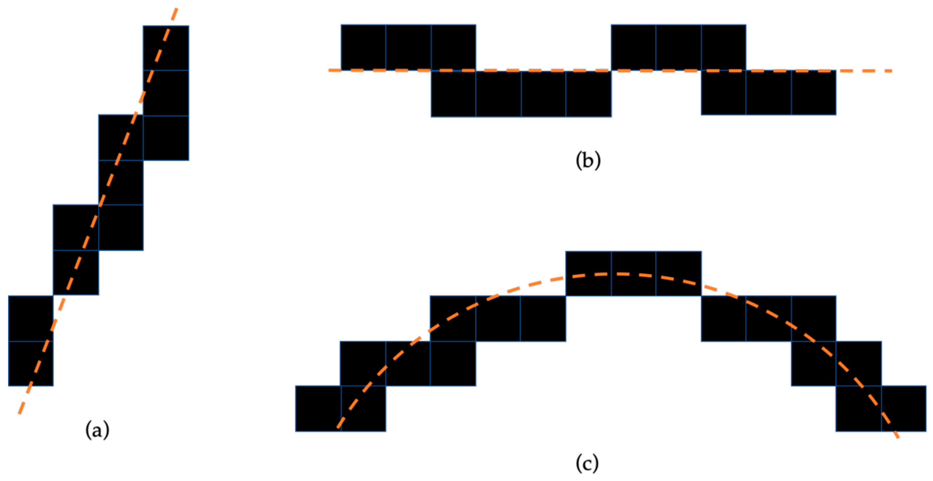
In Canny-processed images, several edge pixels are present in the vicinity of hyperbolic reflections (on prongs and apices): these are useful edge pixels, for the purposes of identifying and characterizing hyperbolas. Further edge pixels are present, which can be considered as noise; some of these pixels, e.g., lay on horizontal reflections generated by the interfaces between different soil layers and by the air–soil interface; for various reasons, there may be further edge pixels that are not in the vicinity of hyperbolic reflections. More specifically, the presence of the following categories of pixel groups was observed in Canny-filtered radargrams:

• Groups of edge pixels that can be fitted by using linear functions with non-zero slope (Figure 3, case a).
• Groups of edge pixels that can be fitted by using linear functions with zero slope (Figure 3, case b).
• Groups of edge pixels that can be fitted by using second-order curves (Figure 3, case c).

Taking these three groups into consideration, the next step of our study consisted in designing a procedure that could be effectively used to segregate only the edge pixels located in the vicinity of the apices of hyperbolic reflections. To achieve this goal, it was decided to consider a small portion of the image around each edge pixel, containing the edge pixel itself and a few pixels in its vicinity. A condition was then sought, to be tested on such image portion, which would be satisfied if the edge pixel under test were located on the apex of a hyperbolic reflection, while it would not be satisfied by an edge pixel positioned on hyperbola prongs, or by an isolated edge pixel. Not only do we need to identify an effective condition but also an appropriate size and shape of the image portion. Edge pixels satisfying the chosen condition would be retained for the next stage of the APEX algorithm, while the other edge pixels would be suppressed.

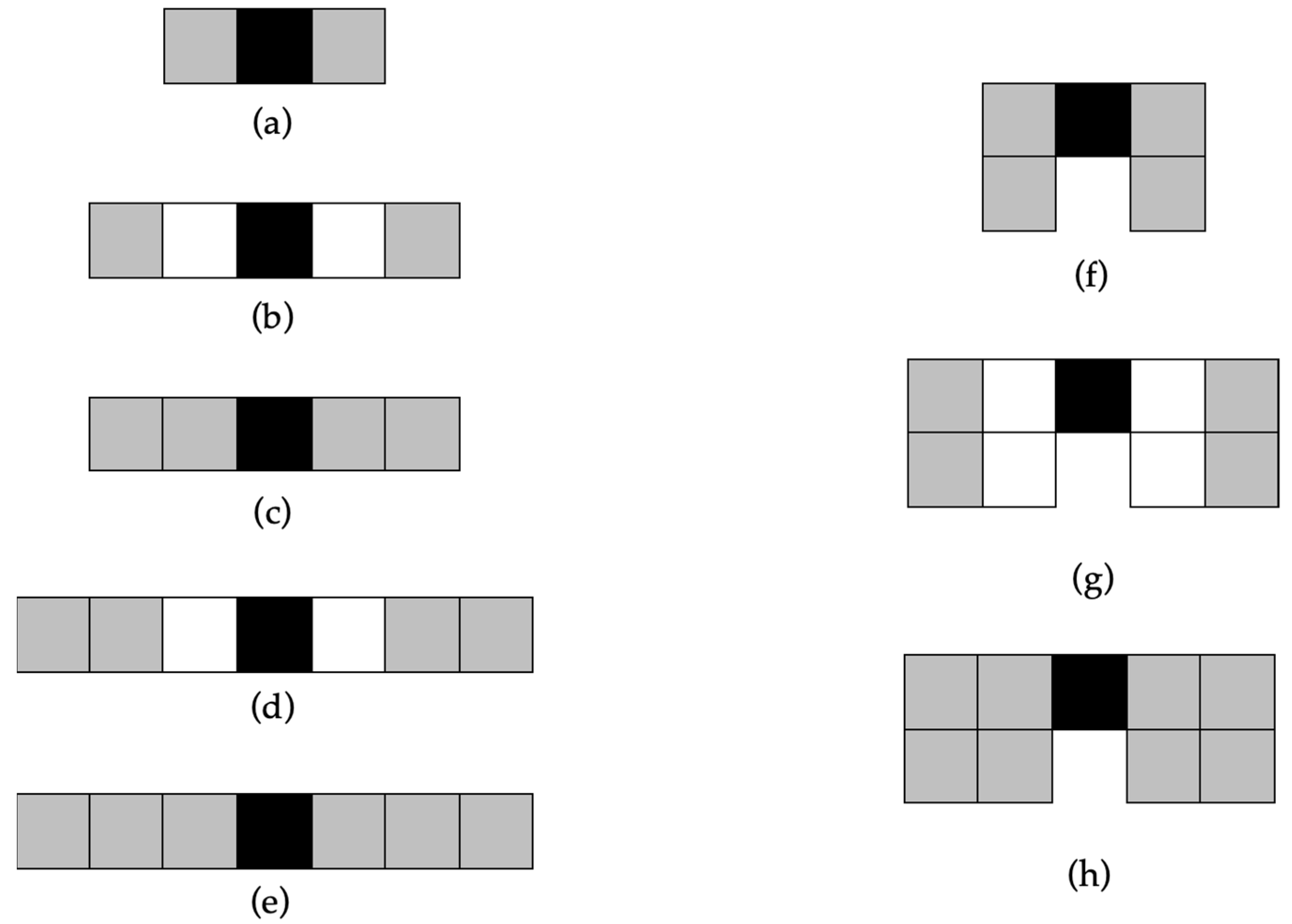
To find an appropriate size and shape of the image portion (hereinafter called “search zone”), the alternatives shown in Figure 4 were considered. In those pixel combinations, the black square is a given edge pixel, grey squares represent pixels included in the proposed search, and white squares represent other image pixels (grey and white squares can, therefore, be edge pixels, or not). From (a) to (e), the search zone extends over a single image line and three to seven columns: in (a) and (b) the number of pixels included in the search zone is the same, but the search zone occupies a wider area in (b); in (c), the search zone extension is the same as in (b), but more pixels are considered; in (d), the number of pixels is the same as in (c), but the search zone is further extended; in (e), the search zone extension is the same as in (d), but more pixels are considered. From (f) to (g), the search zone extends over two image lines and three to five columns: in (f) and (g) the number of pixels included in the search zone is the same, but the search zone occupies a wider area in (g); in (h), the search zone extension is the same as in (g), but more pixels are considered.

Among the combinations depicted in Figure 4, the one to be chosen would meet the following requirements:

• A large number of unwanted edge points is removed from the input dataset.
• Edge pixels located in the vicinity of hyperbolic reflection apices are retained.
• The implemented algorithm is time efficient.
• It is preferable to suppress fewer pixels than to suppress pixels that are useful for identifying apices of hyperbolic reflection.

As far as the condition to be tested on the search zone is concerned, a simple but effective procedure was conceived, which consists in checking whether further edge pixels are present within its search zone. In fact, it is likely that an edge pixel close to the apex of a hyperbolic reflection has at least two edge pixels in its search zone. Absence of further edge pixels in the search zone, most probably implies that the considered edge pixel is not in the vicinity of a hyperbola apex, hence the edge pixel can be removed because it is not useful for the final objectives of the algorithm (hyperbola detection and characterization).

2.4. Experimental and Synthetic Datasets Used to Test the Proposed Algorithms

Numerical tests were performed on 10 synthetic and real radargrams, to verify the effectiveness and performance of the proposed procedure and to identify the most convenient search zone among those depicted in Figure 4. The electromagnetic simulator gprMax [40,56], implementing the finite-difference time-domain technique, was used to generate synthetic radargrams; the experimental radargrams, instead, were recorded in real field surveys carried out in urban areas.

In

Table 1. Fundamental properties of the considered radargrams.

Radargram	Time Samples	Traces	Pixels 1	Experimental or Synthetic	Central Frequency (MHz)
#1	505	120	60,600	Experimental	400
#2	505	372	187,860	Experimental	900
#3	505	584	294,920	Experimental	400
#4	505	688	347,440	Experimental	900
#5	1017	538	547,146	Experimental	900
#6	505	457	230,785	Experimental	500
#7	505	325	164,125	Experimental	400
#8	505	568	286,840	Experimental	400
#9	777	1483	1,152,291	Synthetic	1500
#10	777	1483	1,152,291	Synthetic	1500

¹ Time instants × Traces.

, the basic properties of the considered radargrams are resumed. The smallest one (#1) has 60,600 pixels (120 traces with 505 electric-field amplitudes per trace); the largest radargrams (#9 and #10) have 115,2291 pixels (1483 traces with 777 electric-field amplitude values per trace). The antennas were always ground-coupled, the central frequencies were 400 MHz, 500 MHz and 900 MHz in the experimental cases, 1500 MHz in the simulations.

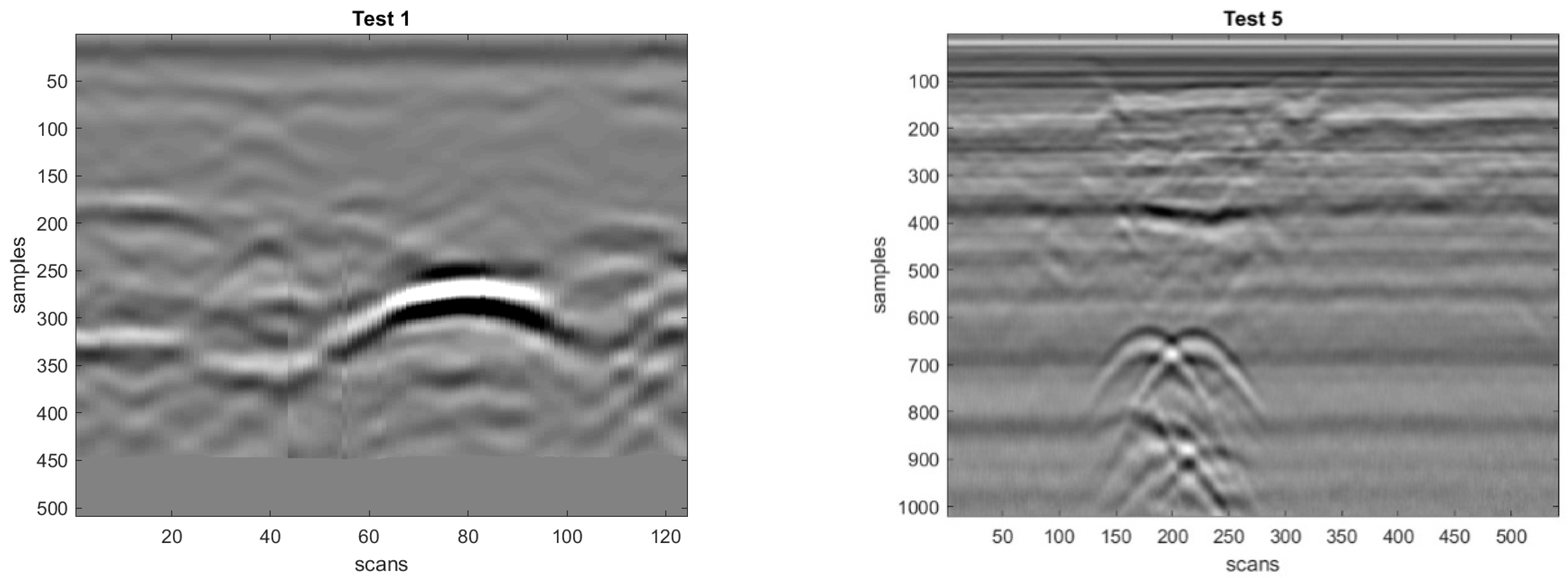
All radargrams are shown in Figure 5 and Figure 6. The eight experimental radargrams presented in Figure 5 were obtained during real GPR surveys carried out in urban areas, in Belgrade, in the presence of different utilities. The two synthetic radargrams of Figure 6 belong to the Open Database of Radargrams of COST (European Cooperation in Science and Technology) Action TU1208 [6], namely Radargram #9 is obtained by scanning Concrete Cell 1.1 proposed in [60], whereas Radargram #10 is obtained by scanning an enlarged version of the same structure [28].

Overall, the considered test radargrams can be divided into three groups:

• Simple radargrams with one hyperbolic reflection (Radargram #1, see Table 1 and Figure 5);
• Medium complexity radargrams, with two or three hyperbolic reflections (Radargrams #2-#5, see Table 1 and Figure 5);
• Complex radargrams with a higher level of noise (Radargrams #6 and #7, see Table 1 and Figure 5) and/or a larger number of reflections (Radargrams #6-#10, see Table 1 and Figure 5 and Figure 6).

In the paper, stronger emphasis is put on experimental data and indeed 80% of test radargrams are experimental.

3. Results and Discussion

The whole procedure outlined in Section 2.3 was applied eight times to every radargram presented in Section 2.4, each time with a different search zone (i.e., overall 80 tests were carried out).

Table 2. Number of edge pixels found in the Canny-processed radargrams.

Radargram	Pixels 1	Edge Pixels
#1	60,600	4564 (7.53%)
#2	187,860	19,909 (10.60%)
#3	294,920	11,445 (3.88%)
#4	347,440	10,312 (2.97%)
#5	547,146	27,044 (4.94%)
#6	230,785	26,987 (11.69%)
#7	164,125	20,271 (12.35%)
#8	286,840	27,492 (9.58%)
#9	1,152,291	77,046 (6.69%)
#10	1,152,291	77,278 (6.71%)

¹ Time instants × Traces.

resumes the number of edge pixels found in every radargram after Canny edge filtering. The smallest radargram (#1) happens to have the smallest number of edge pixels (4564) and one of the two largest radargrams (#10) has the largest number of edge pixels (77,278). The percentage of edge pixels in the various radargrams ranges from 2.97% (radargram #4) to 12.35% (radargram #7), with an average of 7.69%.

In Figure 7, an example is presented, where the procedure described in Section 2.3 is applied to Radargram #8. Showing the complete set of results for every radargram and every search zone would be redundant; since Radargram #8 is among the most complex experimental datasets considered in this paper, the results of Figure 7 are representative enough. In the figure, the edge pixels found by the Canny edge detector are superimposed to the grey-scale map of the original radargram. The proposed procedure for the removal of unnecessary edge pixels is applied by using the eight search zones of Figure 4. The black edge pixels are retained, whereas the red pixels do not satisfy the condition and are removed before sending the radargram to the next steps of the APEX algorithm. A visual inspection of the results presented in Figure 7 reveals that the degree of pixel elimination using search zones (a), (c), (e), (f), and (h) is significantly lower than when search zones (b), (d), and (g) are used. Whether the pixels adjacent to the central one are included or not in the search zone, has turned out to be a distinguishing property that has significant consequences on the number of pixels removed. It can be also appreciated that no edge pixels located in the vicinity of hyperbola apices are removed. This is important for the effectiveness of the subsequent stages of the APEX algorithm, when the exact positions of the apices have to be found. The largest number of eliminated pixels (more than 50% on average) belong to the hyperbola prongs and to other irregular reflections or noise existing in the radargram considered.

The results obtained for the other radargrams are rather consistent with those presented in Figure 7. From a careful analysis of all the results obtained, we have observed that the only “error” (i.e., removal of useful pixels) occurred when processing Radargram #7 by using search zone (b): in that unfortunate case, all pixels in the vicinity of a hyperbola apex were removed. For this reason, we think that search zone (b) should not be used. Search zones (d) and (g) appear to be more robust than (b), and this is obviously due to the fact that they include a higher number of pixels; at the same time, they are more effective than search zones (a), (c), (e), (f), and (h), which produce the removal of a number of pixels that is too low for our purposes.

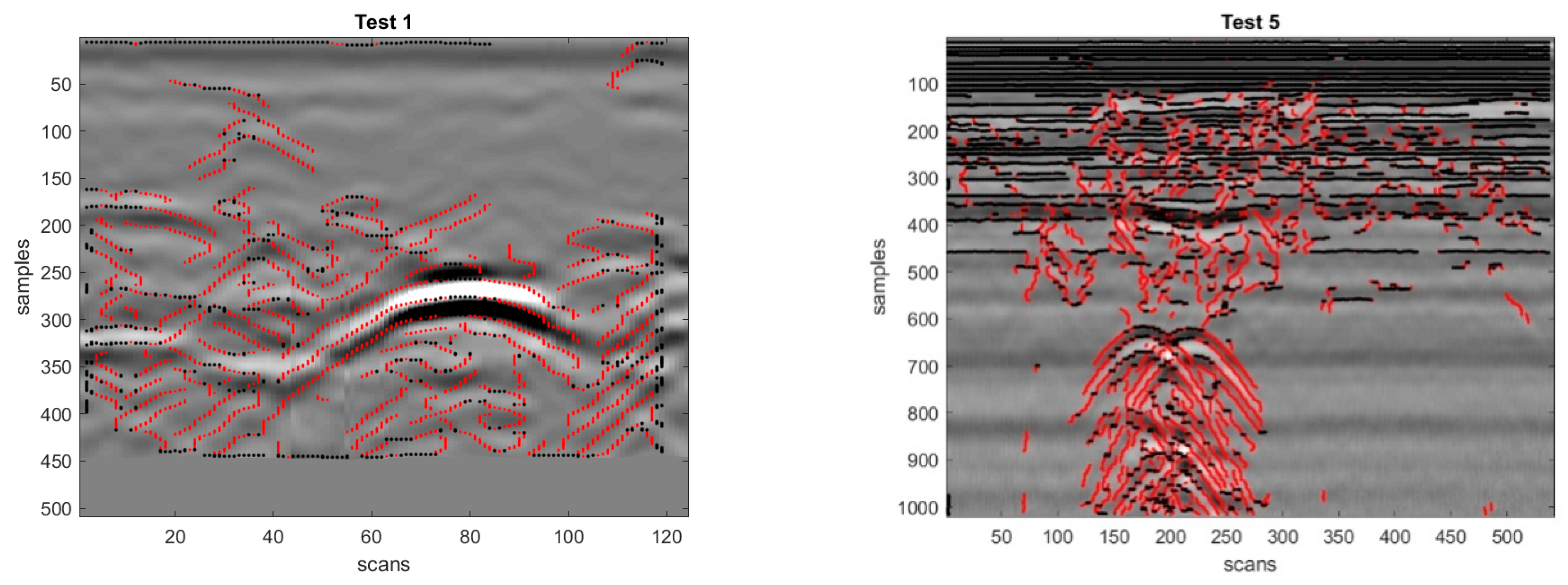
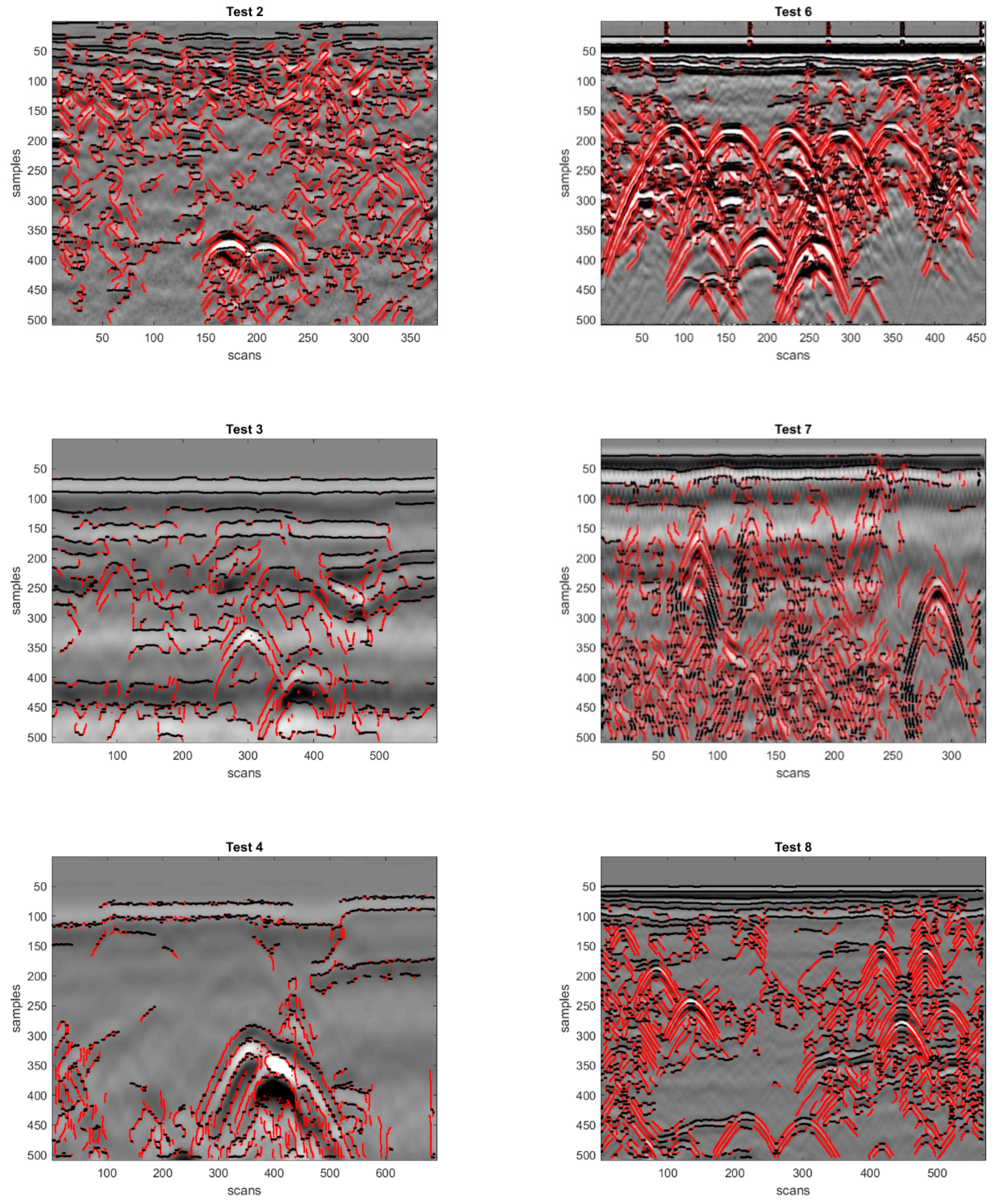
In Figure 8, the edge removal results obtained for the eight experimental radargrams by using search zone (d) are presented (obviously, the bottom right image included in this figure is identical to Figure 7d). In Figure 9, the same as in Figure 8 is presented for the two synthetic radargrams. Based on the tests that we have carried out so far, we think that search zone (d) can be considered as the best solution (search zone (g) does not seem to yield advantages compared to (d), and being larger it implies a slightly longer execution time). We plan to carry out additional tests with other radargrams in the near future, to further consolidate this conclusion.

We have also noted that the edge pixels originated from horizontal reflections always remain in the radargrams (see, e.g., Radargram #5 in Figure 8, or Radargrams #9 and #10 in Figure 9). For the removal of such edge pixels, we envisage to conceive and implement a dedicated procedure in the near future.

Figure 10 shows the percentage of edge pixels removed by the procedure presented in Section 2.3, for all the considered radargrams and all the search zones. Figure 11 shows the processing time for all the considered radargrams and all the search zones.

By observing Figure 11, it is apparent that the smallest search zones (a) and (b) correspond to the shortest execution times, while the execution of the procedure takes a slightly longer time when a wider search zone is used (as expected). However, it can be noticed that there are no significant differences in terms of execution time when different search zones are used, especially for radargrams that contain a not too high number of edge pixels. The processing time is longer in the presence of a higher number of edge pixels in the Canny processed radargram; usually, larger radargrams contain a higher number of edge pixels (as shown in Table 2). The average processing time for the search zones that remove the highest number of pixels are: 0.01 s, 0.08 s, and 0.14 s, respectively, for search zones (b), (d), and (g). It has to be mentioned that the processing time plotted in Figure 11 includes the Canny edge detection, as well. If this process would be excluded, the time would decrease of approximately two thirds; i.e., the application of the procedure for the removal of unwanted edge pixels takes about one third of the time shown in Figure 11. Since the maximum processing time is less than half a second, it can be concluded that the proposed processing approach is an excellent candidate to become the initial stage of an upgraded version of APEX, which will be capable of yielding results in near real-time. To calculate the processing time shown in Figure 11, the embedded MATLAB function etime was used.

Concerning the search for pixels lying on hyperbola prongs (see Section 2.1), it is worth pointing out that the procedures presented in this paper (i.e., Canny edge filtering followed by removal of unnecessary edge pixels) are used to extract pixels that are in the vicinity of hyperbola apices and to estimate the coordinates of the apices in near real time. The removed pixels of course include many prong pixels, as it should be (see Figure 7, Figure 8 and Figure 9). When the hyperbola apices are found, and the targets are therefore detected and localized, the execution of APEX can continue with an analysis of further hyperbola properties. In particular, if there is an interest into estimating the target size and/or the soil relative permittivity, APEX can perform a tracing of the hyperbola prongs. This task is fulfilled on the entire original radargram, not on the Canny processed one, in the same manner as was done in the original version of APEX.

For the sake of completeness, an example of detection, localization and prong tracing results obtained by using APEX is now presented. In

Table 3. Coordinates of hyperbola apices (in terms of pixels) found in Radargram #8 by using the original and upgraded versions of the APEX algorithm.

Hyperbola Apex	Apex Coordinates
	Original Algorithm	Upgraded Algorithm
1	Row: 122 Column: 35	Row: 118 Column: 35
2	Row: 158 Column: 419	Row: 154 Column: 418
3	Row: 160 Column: 486	Row: 156 Column: 484
4	Row: 190 Column: 85	Row: 185 Column: 84
5	Row: 243 Column: 137	Row: 238 Column: 135
6	Row: 280 Column: 450	Row: 275 Column: 449
7	Row: 257 Column: 514	Row: 253 Column: 513
8	Row: 436 Column: 219	Row: 432 Column: 218
9	Row: 444 Column: 305	Row: 440 Column: 304

, the coordinates of the hyperbola apices found by APEX in Radargram #8 are reported in terms of image pixels; results obtained with the original and upgraded versions of APEX are compared (for the upgraded version of the algorithm, search zone (d) was used). First of all, it can be noticed that both versions of the algorithm detected nine apices. The horizontal coordinates of the apices are almost the same (i.e., the column values, which indicate the spatial position along the radar acquisition line): in fact, the absolute difference between original and new results is between 0 and 2 pixels. As far as the vertical coordinates of the apices are concerned (i.e., the row values, which indicate the position along the time axis), the absolute difference between original and new results is between 4 and 5 pixels. Since the time window for this radargram is 56 ns and the number of rows is 505 (Table 1), one pixel corresponds to 0.11 ns. In Figure 12, the apices found by the new version of APEX are represented by green dots and superimposed to Radargram #8; moreover, the black pixels are the hyperbola prongs traced by APEX. This figure clearly illustrates the effectiveness and accuracy of the algorithm.

Finally, we would like to emphasize some less evident advantages arising from the introduction in APEX of the Canny edge detector followed by the procedure for the removal of unnecessary edge pixels.

We have already mentioned how the use of the procedures presented in this paper is useful to accelerate the execution of APEX and obtain near real-time results, since the search for hyperbola apices is performed on a smaller number of pixels. However, there is more. In particular, thanks to the introduction of these procedures in APEX, the overall algorithm becomes fast enough to make it possible to avoid the use of a trained neural network to find the SOIs (see Section 2.1). In fact, it is envisaged that in the final version of the upgraded APEX the hyperbola detection algorithm will be run over the entire radargram, directly (after Canny edge filtering and removal of unnecessary pixels), not only on the SOIs. In this way, the upgraded APEX will become more robust than the original APEX, especially in the presence of interfering targets and highly complex radargrams. In this regard, it is worth noticing that, in the original version of APEX, false positive detections of SOIs may occur, as well as failures to detect actual SOIs (i.e., false negative detections of SOIs). In fact, based on our experience, it is not realistically possible to create a universal training set for the neural network, which would provide excellent and uniform results for all possible input data (taking into account all possible kinds and dimensions of utilities, burial depths, soil properties and structures, various effects due to the electromagnetic interference between adjacent targets, etc). While the false positive detections of SOIs in the original version of APEX are not a big problem, because they are normally overrun in the subsequent stages of the algorithm, the false negative detections have a negative impact on the accuracy of the algorithm. In particular, whenever an existing hyperbolic reflection is not detected by the trained neural network, as a consequence the relevant target cannot be localized and registered by APEX. By avoiding the use of a trained neural network, this problem can be overcome.

Another advantage of using the Canny edge detector is that APEX becomes less susceptible to noise, which is especially important in the context of GPR and through-the-wall applications, as evidenced by the significant efforts being made by various research teams to reduce clutter levels in surface penetration radar data [61,62,63].

In a future work, specific examples will be presented to highlight and demonstrate these advantages.

4. Conclusions

The research work presented in this paper investigated the use of the Canny edge detector in the initial stage of APEX (automated point extraction from radargrams), a previously proposed advanced algorithm for the automatic detection and characterization of hyperbolic reflections in ground-penetrating radar (GPR) radargrams. The implementation solution described in this paper largely decreases the number of unnecessary edge pixels in Canny edge processed radargrams and correctly retains edge pixels that are in the vicinity of hyperbolic reflections’ apices.

The procedures presented herein have been successfully tested over eight experimental and two synthetic radar images with different levels of complexity and noise, obtained with antennas working at various central frequencies ranging from 400 MHz to 1.5 GHz. Based on the promising findings of this study, the introduction of the new procedures into APEX has proved to be a robust upgrade of the algorithm, which is extremely useful for reducing its overall execution time. To further improve this upgrade of APEX and make the algorithm even faster, future steps will include the implementation of suitable procedures to remove also the unnecessary edge pixels originating from horizontal reflections (e.g., due to road and soil layers) and the definition of additional criteria to eliminate other unwanted edge pixels (e.g., due to noise and small reflections generated by debris or stones in the soil). Finally, only the edge pixels in the vicinity of the apices of hyperbolic reflections will be retained for the purposes of estimating the coordinates of the apices.

It is worth emphasizing that the original version of the APEX algorithm makes use of a trained neural network to identify the so-called “segments of interest”, i.e., small regions of the radargram under test containing the sought objects (hyperbolas). The final version of the upgraded APEX will be made independent of the use of a trained neural network, and this is expected to increase its effectiveness and accuracy. The upgraded algorithm will provide results in near real-time and, thanks to the use of the Canny operator, it will also be less susceptible to noise than the original algorithm.