Abstract
Intelligent anomaly detection is a promising area to discover anomalies as manual processing by human are generally labor-intensive and time-consuming. An effective approach to deal with is essentially to build a classifier system that can reflect the condition of the infrastructure when it tends to behave abnormally, and therefore the appropriate course of action can be taken immediately. In order to achieve aforementioned objective, we proposed to build a dual-staged cascade one class SVM (OCSVM) for water level monitor systems. In the first stage of the cascade model, our OCSVM learns directly on single observation at a time, 1-g to detect point anomaly. Whereas in the second stage, OCSVM learns from the constructed n-gram feature vectors based on the historical data to discover any collective anomaly where the pattern from the n-gram failed to conform to the expected normal pattern. The experimental result showed that our proposed dual-staged OCSVM is able to detect anomaly and collective anomalies effectively. Our model performance has attained remarkable result of about 99% in terms of F1-score. We also compared the performance of our OCSVM algorithm with other algorithms.
1. Introduction
Anomaly detection has been playing a very crucial part in large industries like gas, oil, power plant, water, and telecommunication system. Effective anomaly detectors are capable of picking up subtle unusual behaviours or abnormal data patterns which are not supposed to occur under normal operating conditions [1]. These anomalies can be caused by malicious attacks in the physical environment, unintentional human factors, bugs in the system’s components, etc. Therefore, we need to facilitate the process of development, maintenance and overhaul when certain events are seen abnormal. These research areas have been widely studied and discussed in [2,3,4,5].
Any anomaly pattern detected in the water level system such as substantial surge, abrupt decline, stagnated level or any patterns deviated significantly from the normal behaviour have to be captured and flagged out instantly in the anomaly detection system. However, manual examinations by human are generally labor-intensive and time-consuming, thus smart effective diagnosis on these anomalies is extremely imperative [6]. Coupled with anomaly detection system, a proactive course of action can be taken to remedy the anomalies in the early stage. Not only does it enhance the reliability of the system under monitoring, but it also reduces the costs for the overhaul of the infrastructure.
Although many classification problems have been dealing with two or more classes, some real-world issues like anomaly detection are best devised as one-class classification approach. These one-class classifiers are trained mostly with majority class and never encounter those from the minority class. Hence, it has to estimate a decision boundary which can separate the minority class from the majority class. This paper presents an unsupervised machine learning approach called one-class support vector machine in a dual-staged cascade to discover the anomalies in the water level system.
2. Materials and Methods
An anomaly detector provides an efficient way to detect anomalous behaviors based on the analysis of traffic patterns of the water level traffic data. It can be used to evaluate whether the scenarios or situations are under non-optimal operating conditions. Anomalous behaviors essentially indicate that the current water level deviates from the norm. The ability to discover such behaviors in the infrastructure application is non-trivial as the impact of an abnormal water supply to the infrastructure can be potentially severe. The deployment of an anomaly detector on water level systems is paramount because it can fix the vulnerability of being attacked or failing.
2.1. Data Description
We used water level traffic datasets from an IT-based infrastructure company, Infranics, located in the capital of South Korea. Infranics gathers a stream of data which are generated from several sensor devices and provides solutions like intelligent safety diagnosis and disaster prediction services for safety management on underground communication systems. In this paper, the data we were dealing with were obtained from water tank level sensors. The sensors were wired on the surrounding of the infrastructure in order to attain a real-time reading of the water level. Our acquired data were a complete one-day operative data which were captured at a 1 Hz sampling rate. It had both the minimum and maximum threshold for the inflow and outflow of the waterworks. Other than identifying the anomalous behavior of the water going beyond those thresholds, we also needed to identify the peculiar behaviors that did not conform to the expected patterns.
2.2. Artificial Data Generation
Since we had a data stream containing only the normal class (majority class), we deliberately injected some amount of abnormal class (minority class). In order to learn the latent patterns of the water level, we adopted autoencoder [7]. It essentially tries to learn the identity function and makes predictions of future patterns. The predicted patterns will be subsequently transformed with the scaling factor and treated as abnormal class.
Autoencoder is made up of two neural networks, namely encoder and decoder. In the encoder network, it learns from the input data, x, and constructs an encoded representation via a function. Whereas the decoder will reconstruct the data, , as close as to the input data, x, given the encoded representation. Figure 1 illustrates how an autoencoder works.
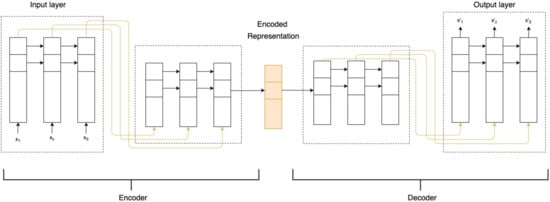
Figure 1.
Illustration of the LSTM autoencoder.
More specifically, the input normal data is being normalized and reshaped into a 3-dimensional array (numSample, timestep, numFeature) before feeding into the encoder layer of an autoencoder. We explain the terminology in the aforementioned array: numSample denotes the total number of training data observations in one time step, timestep denotes the number of observations at each time step, and lastly numFeature indicates the number of features in the dataset, where the feature is the water level itself. An encoded feature will be extracted and compressed by going through the LSTM hidden layer of our autoencoder. Subsequently, the decoder reconstructs the water level pattern to be mostly normal based on the reconstruction probability. We minimize the reconstruction error with the objective function as shown in Equation (1).
We process the output of the decoder layer with a scaling factor, to generate the anomalous data. The mixture of both normal and anomalies will be fed as the input data for the dual-staged cascade one class support vector machine (OCSVM) system. We designed our system flow in two stages. The former stage detects the point anomalies via 1-g as the feature vector in the data instances. It analyses the water level system whether any specific components are performing within the optimal operating range. Subsequently, in the latter stage, the algorithm constructs a sliding window from the historical data and learns n-gram feature vectors to detect collective anomalies. This is to identify an unexpected or abnormal manner based on the historical data.
2.3. One-Class Classifier
Support vector machine, also known as SVM [8,9] was a learning technique based on the principle of structural risk minimization from statistical learning theory. The idea was first introduced to solve classification problems on two classes. It was also devised and adapted to handle one-class classification problems by [10,11,12].
2.3.1. Support Vector Data Description
Support vector data description (SVDD) [12] is an algorithm which creates a hypersphere in the high-dimensional space. Given a set of data points, the hypersphere defined by the algorithm can encompass the data. Therefore, it is able to separate the data points from the outliers and discover the anomalies. SVDD has been widely practiced in handwritten digit recognition, face recognition and anomaly detection. Its mathematical function is expressed as follows:
where R and a denote radius and centre of the hypersphere respectively, C is a hyperparameter that controls the number of data points falls outside the hypersphere, whereas denotes a mapping function to high dimensional space, and represents a slack variable.
2.3.2. One-Class Support Vector Machine
In our work, we employ one-class support vector machine and build it in two stages. We are going to use one-class information (normal class) to learn a classifier that is potential to identify instances belonging to its own class and rejecting unseen classes as outliers. The OCSVM algorithm was implemented using scikit-learn library [13], which was based on LIBSVM [10]. Assume , where , and consider every instances from the training set are distributed under a certain probability distribution, P. We want to find if the instances from testing set are distributed according to the distribution of training set, P. A region of feature space will be determined in such a way that the probability of the test instance being drawn from P falls outside of that region is confined by a specific parameter, . Thus, the decision function is estimated to infer the instances within the region to be positive and negative elsewhere.
The input data are transformed into a high-dimensional space from the original space via a non-linear kernel function. Therefore in this case, one-class SVM algorithm creates a decision boundary in the high-dimensional space and linearly separates the data points with the outliers. Its quadratic equation [14] is expressed as follows:
where is a parameter controls the upper bound for the outliers, is an offset that characterizes a hyperplane , represents a mapping function and denotes a slack variable.
We apply radial-basis function (RBF) kernel for our algorithm, as shown in Equation (2). It is primarily because RBF can create a non-linear curve that encompasses the data well. Thus it is able to identify any outliers in the original space. The data points belonging to normal class will lie within the boundary, whereas the abnormal class will be on the other side. We performed OCSVM on the data with different parameters, , to evaluate the accuracy performance of our model. The mathematical expression for RBF is given as:
where is L2 norm of two feature vectors (i.e., x and ) and is a parameter that controls deviation of the kernel function.
As the input data of our water level system is time series data (which incorporates temporal dependence among the elements), we employ sliding window approach [15] to transform data into n-gram feature vectors. Let as t-th input sequence of the data points and n as the size of the sliding window, then we obtain a set of window, . Take 3-g, for example—if the water level dataset has the sequence of {2, 3, 4, 6, 3, 1}, then the set created from this sequence would be {(2, 3, 4), (3, 4, 6), (4, 6, 3), (6, 3, 1)}. These n-grams form a set of feature vectors for the water level dataset. The sliding window of fixed size n will be progressively slid across the entire input sequence from the beginning till the end to construct a bag of n-gram feature vectors [16,17], as illustrated in Figure 2. One-class SVM classifier will label the window as a whole to be abnormal if there is at least one input instance lies as an outlier, otherwise it will be labeled as normal. Given the data points, the aim of the machine learning algorithm is to generate a hypothesis that estimates the inference, , where denotes the corresponding class label with +1 as “normal” and −1 as “abnormal”.
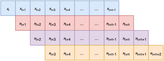
Figure 2.
Illustration of n-gram feature vectors.
Together, we have a dual-staged cascade one-class support vector machine (OCSVM) by making use of both 1-g and n-gram feature vectors. The overall architecture of our proposed method is illustrated in Figure 3. The former identifies a particular data point that deviates significantly from the normal data pattern, whereas the latter implies a collection of data in a consecutive time intervals which behaves anomalously with respect to the entirety of the data stream. The goal is to detect both point anomalies, such as an abrupt change between and , and collective anomalies like a peculiar pattern within a specified window.
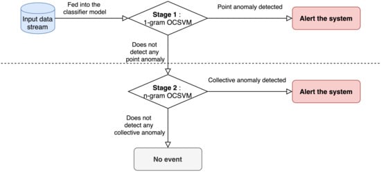
Figure 3.
Architecture of dual-staged cascade one class support vector machine (OCSVM).
During the first stage of the cascade model, the learning algorithm fits OCSVM model from point observation and the generated OCSVM detects if particular data instance is outlier—this stage is called point anomaly detection stage. For the second stage, the observational data is constructed into n-gram feature vectors and fed into the SVM learning algorithm to learn OCSVM model for them. The generated classifier predicts whether a given n-gram feature is an outlier or not. The purpose of building this second stage is to manage the continuous pattern of water level, so that any peculiar behavior failed to discover in point anomaly detection stage can be detected—this stage is called the collective anomaly detection stage. A more in-depth explanation will be described in Section 3.
2.4. Evaluation Metric
In order to monitor the performance of our proposed system, we generate a confusion matrix from our experimental results. For our anomaly detection problem, we form a 2 × 2 confusion matrix as shown in Table 1. It computes the number of true positive (TP), false positive (FP), false negative (FN), and true negative (TN) results.

Table 1.
The illustration of the confusion matrix for binary classification problem. a, b, c, and d denotes the number of true positive (TP), false negative (FN), false positive (FP) and true negative (TN), respectively. TP: actual class, anomaly (True = Yes) and prediction class, anomaly (True = Yes); FN: actual class, anomaly (True = Yes) and prediction class, normal (False = Yes); FP: actual class, normal (False = Yes) and prediction class, anomaly (True = Yes); TN: actual class, normal (False = Yes) and prediction class, normal (False = Yes).
From the confusion matrix, we can compute the score of precision and recall, as shown in Equations (3) and (4) respectively.
Moreover, F1-score in Equation (5) is described as a harmonic mean of precision and recall [18]. Its mathematical formula is derived as below:
3. Experiments
First of all, we partitioned our entire dataset (as shown in Figure 4) to form a training set and a testing set with the ratio of 70:30. In other words, the classifier is trained with novelty data (70% of the dataset) and the rest, 30% of the dataset will be held out from the entire dataset for testing our trained one-class SVM model. The training set contains only normal data, whereas the testing set is comprised of mixture of normal and abnormal data.
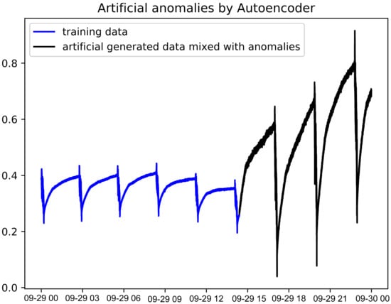
Figure 4.
Illustrated graph of the water level dataset after mixing with artificial anomalous data.
One-class SVM infers each of observational data as +1 or −1 to tell whether does it belong to inlier or outlier respectively. For the evaluation of our model performance, we compare the predicted label against the defined ground truth label. To demonstrate the practical effectiveness of the anomaly detection system, we deployed our dual-staged cascade one-class SVM model to the web framework via Flask REST API.
In our dual-staged cascade system, we designed our classifier in an optimized manner. First, our anomaly detection model treats every single input data as an individual feature vector and evaluates them in discrete point form. Next, the second stage reconstructs the dataset into n-gram feature vector, where n = {60, 120, 180, 300}, which spans over 1 min, 2 min, 3 min and 5 min, respectively, in our designed system. The choice of having this window size is to enable the system to learn the pattern and discover the anomalies in a short turnaround time. Note that overly large window size tends to increase the chances of being overfitted. A group of n-grams feature vectors is created through fixed-size sliding window from the input data and fed into the model for inference. The model receives the data in JSON format and makes inference on them to decide whether it is normal or abnormal. We proposed this dual-staged anomaly detection system to discover these point anomalies and collective anomalies [19] in the water level monitoring system.
We employed the RBF kernel (based on Equation (2)) in our dual-staged one-class SVM classifier and experimented with two different parameters, which are n, and . The former denotes the size of the sliding window whereas the latter, parameter, is known as an upper bound for the outliers—it controls the compromise between the mislabeled normal class and the vector-norm of the learned weight. We ran a grid search method on these parameters to choose the best combination with respect to F1-score.
4. Results
4.1. Data Preparation
Data Preparation and Preprocessing
Before feeding the data to train the classifier model, it is vital to preprocess the raw data. The performance of the classifier model boils down to the data preprocessing. Since not all of the data collected are useful, we need to perform important steps such as data cleaning, data transformation and noise identification beforehand. After that, we extract the appropriate features from the raw data which gives significant impact on the performance of machine learning algorithm. It is because constructing an appropriate number of gram on the dataset will impact the experimental results as it is time-dependent.
4.2. Experiment Result
We have used test data containing 34,400 observations to evaluate the performance of the model. We have explored different parameters with the combination of and to attain the optimal performance result. Table 2 summarizes the result for the one-class SVM classifier on the water level anomaly detection with respect to precision, recall and F1-score, according to Equations (3)–(5). The precision, recall and F1-score on the 1-g and n-gram one-class support vector machine have been computed to assess their model performance.
Table 2.
Precision, recall, and F1-score of different gram and parameters on OCSVM. Best performance of the F1-score is highlighted in bold.
5. Discussion
Table 2 presents the results of the dual-staged one-class SVM by varying different parameters, n and . We focus on improving the F1-score by performing a series of experiments on these parameters. High value of F1-score describes the model has the best possible performance given with the optimal parameter values.
As we can see from Table 2, the model achieved the highest F1-score of 99.48% with configuration of = 0.25 on 1-g. On the subsequent stage for 60-g in Table 2, it attained a F1-score up to 98.55% at = 0.25. We can conjecture that it can detect the anomalous behavior effectively in the 1-min trend window, although there might trigger minor amount of false alarms sporadically. Generally, it still showed relatively high precision and recall score. Our OCSVM model of 300-g configuration achieved even higher F1-score than the models with 60-g, 120-g and 180-g. We can clearly observe that it has 99.06% at = 0.3, which was quite satisfactory. It reduced the rates of false positives and false negatives. The comparison of dual-staged OCSVM on 60-g, 120-g, 180-g and 300-g is illustrated in Figure 5a–d. As shown in Figure 5, 600-g OCSVM was able to detect more anomalies and trigger less false alarm compared to those of 60, 120, and 180-g collectively.
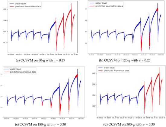
Figure 5.
Comparison of dual-staged one-class SVM on the anomaly detection.
Besides, we experimented additional techniques like sampling technique to study the inference on the population. Two different sampling methods we used are average sampling and random sampling. Each instance was sampled averagely or randomly from every 60-observations interval window to form a set of observational data. According to the Figure 6a,b, the performance results were not that satisfactory as the population had been significantly down-sampled. It could only detect a handful of anomalous data due to the sparse filtering. Another factor that led to poor performance was attributed to the small training dataset.
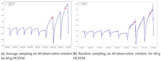
Figure 6.
Comparison of sampling techniques (average and random) of 60-observations window on the population.
We also performed a series of experiments with SVDD algorithm [12] to compare the performance with dual-stage OCSVM system. For fair comparison with our OCSVM which is based on LIBSVM, we adopted SVDD extension of LIBSVM. Table 3 illustrates the precision, recall and F1-score evaluated with various values of C parameter. On the first stage for 1-g, the model showed the F1-score of 94.04% when the parameter C = 0.0001, whereas on the subsequent stage for 60-g, 120-g, 180-g and 300-g, the F1-score gave the highest F1-scores of 92.75%, 93.56%, 92.82% and 92.88% respectively. Figure 7 illustrates the comparison of SVDD of different n-gram = {60, 120, 180, 300}. It can be clearly seen that their results were pretty much comparable among each other and there exists a certain amount of false alarms. In overall, we conjectured OCSVM algorithm outperforms SVDD in our water level anomaly detection task.
Table 3.
Precision, Recall, F1-score of different grams on SVDD algorithm. Best performance of the F1-score is highlighted in bold.
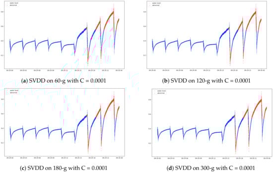
Figure 7.
Comparison of support vector data description (SVDD) anomaly detection on different gram configurations.
It should also be noted that we compared our method with two other different algorithms—Elliptic Envelope and Isolation Forest. What the Elliptic Envelope algorithm does is that it assumes the data is drawn from a Gaussian distribution and the shape is defined based on the data distribution. Any instances which lie outside the variance will be treated as outliers. Isolation Forest, on the other hand, performs random partition on the data instances and computes the split value between the maximal and minimal value of the selected observation. Instances will be classified as anomalies if and only if the path length of the partitioned observation is short.
From the results in Table 4, it was worth noting that one-class SVM has achieved outstanding result over those of using Elliptic Envelope and Isolation Forest. We made the comparisons in the aspect of precision and recall, finding that one-class SVM obtained the best performance result among them. It has emitted lesser false positives and false negatives than the other two algorithms. Elliptic Envelope algorithm has appeared to be have high rate of false negatives and led to unsatisfactory performance. The performance on Isolation Forest algorithm is promising when it is evaluated with 1-g configuration. However, as the n-gram grows larger, we noticed that precision and recall have started to degrade, with more and more data instances being misclassified. Our dual-staged cascade system built with OCSVM algorithm still generally outperforms these two algorithms.
Table 4.
Comparison of Elliptic Envelope, Isolation Forest and one-class SVM algorithms. Best performance is highlighted in bold.
6. Conclusions
In this work, we have presented our method—dual-staged cascade OCSVM for anomaly detection on water level system. It comprises of two stages, the first one detects any point anomalies by running 1-g on the observational data, and the subsequent stage runs n-gram to identify collective anomalies in the broader perspective. We tuned the parameters of the model and the window size configuration to seek for the best performance out of the model. Our dual-staged OCSVM technique achieved excellent result of 99.06% F1-score with the parameter = 0.3. Other than that, additional comparison with other algorithms like SVDD, Isolation Forest and Elliptic Envelope were evaluated. Our implemented technique has outperformed those state-of-the-art algorithms in this application. It was thus found that our proposed dual-staged OCSVM technique can detect different kinds of anomalies in different scenarios effectively. The use of dual-staged technique is able to isolate both point anomalies and collective anomalies, and therefore gives higher yield.
In our future work, we plan to explore and extend our study in several directions. First of all, we are actively doing research to further enhance and increase our model performance. In addition, we need to investigate on more corner cases as the dataset we used contains deliberately injected anomalies. Different anomalies should have their distinct characteristic for the classifier model to detect.
Author Contributions
Conceptualization, F.H.S.T. and D.-K.K.; Data curation, J.R.P.; Formal analysis, F.H.S.T. and D.-K.K.; Funding acquisition, D.-K.K., K.J. and J.S.L.; Investigation, J.R.P.; Methodology, D.-K.K.; Project administration, D.-K.K., K.J. and J.S.L.; Resources, J.R.P.; Software, F.H.S.T.; Supervision, D.-K.K.; Validation, D.-K.K., J.R.P., K.J. and J.S.L.; Visualization, F.H.S.T.; Writing—original draft, F.H.S.T.; Writing—review & editing, D.-K.K. All authors have read and agreed to the published version of the manuscript.
Funding
This research was supported by the MSIT (Ministry of Science, ICT), Korea, under the IISD (Intelligence Information Service Diffusion) support program (NIPA-2019-A0602-19-1050) supervised by the NIPA (National IT Industry Promotion Agency).
Acknowledgments
The authors wish to thank members of the Dongseo University Machine Learning/Deep Learning Research Lab., members of Infranics R&D Center at Infranics Co., Ltd., and anonymous referees for their helpful comments on earlier drafts of this paper.
Conflicts of Interest
The authors declare no conflict of interest.
Abbreviations
The following abbreviations are used in this manuscript:
| SVM | Support Vector Machine |
| OCSVM | One Class Support Vector Machine |
| RBF | Radial Basis Function |
| SVDD | Support Vector Data Description |
| DOAJ | Directory of open access journals |
References
- Chandola, V.; Banerjee, A.; Kumar, V. Anomaly detection: A survey. ACM Comput. Surv. 2009, 41, 15:1–15:58. [Google Scholar] [CrossRef]
- Jones, A.; Kong, Z.; Belta, C. Anomaly detection in cyber-physical systems: A formal methods approach. In Proceedings of the 53rd IEEE Conference on Decision and Control, Los Angeles, CA, USA, 15–17 December 2014; pp. 848–853. [Google Scholar] [CrossRef]
- Harada, Y.; Yamagata, Y.; Mizuno, O.; Choi, E. Log-Based Anomaly Detection of CPS Using a Statistical Method. In Proceedings of the 2017 8th International Workshop on Empirical Software Engineering in Practice (IWESEP), Tokyo, Japan, 13 March 2017; pp. 1–6. [Google Scholar] [CrossRef]
- Inoue, J.; Yamagata, Y.; Chen, Y.; Poskitt, C.; Sun, J. Anomaly Detection for a Water Treatment System Using Unsupervised Machine Learning. In Proceedings of the 2017 IEEE International Conference on Data Mining Workshops (ICDMW), New Orleans, LA, USA, 18–21 November 2017; pp. 1058–1065. [Google Scholar] [CrossRef]
- Li, Z.; Li, J.; Wang, Y.; Wang, K. A deep learning approach for anomaly detection based on SAE and LSTM in mechanical equipment. Int. J. Adv. Manuf. Technol. 2019, 103. [Google Scholar] [CrossRef]
- Lei, Y.; Jia, F.; Lin, J.; Xing, S.; Ding, S. An Intelligent Fault Diagnosis Method Using Unsupervised Feature Learning Towards Mechanical Big Data. IEEE Trans. Ind. Electron. 2016, 63. [Google Scholar] [CrossRef]
- Kramer, M.A. Nonlinear principal component analysis using autoassociative neural networks. AIChE J. 1991, 37, 233–243. [Google Scholar] [CrossRef]
- Vapnik, V. Statistical Learning Theory, 1st ed.; Wiley-Interscience: New York, NY, USA, 1998. [Google Scholar]
- Cortes, C.; Vapnik, V. Support-Vector Networks. Mach. Learn. 1995, 20, 273–297. [Google Scholar] [CrossRef]
- Chang, C.C.; Lin, C.J. A Library for Support Vector Machines. Available online: http://www.csie.ntu.edu.tw/~cjlin/libsvm (accessed on 11 September 2019).
- Schölkopf, B.; Platt, J.C.; Shawe-Taylor, J.C.; Smola, A.J.; Williamson, R.C. Estimating the Support of a High-Dimensional Distribution. Neural Comput. 2001, 13, 1443–1471. [Google Scholar] [CrossRef] [PubMed]
- Tax, D.M.; Duin, R.P. Support Vector Data Description. Mach. Learn. 2004, 54, 45–66. [Google Scholar] [CrossRef]
- Pedregosa, F.; Varoquaux, G.; Gramfort, A.; Michel, V.; Thirion, B.; Grisel, O.; Blondel, M.; Prettenhofer, P.; Weiss, R.; Dubourg, V.; et al. Scikit-learn: Machine Learning in Python. J. Mach. Learn. Res. 2011, 12, 2825–2830. [Google Scholar]
- Schölkopf, B.; Williamson, R.; Smola, A.; Shawe-Taylor, J.; Platt, J. Support Vector Method for Novelty Detection. In Proceedings of the 12th International Conference on Neural Information Processing Systems (NIPS’99); MIT Press: Cambridge, MA, USA, 1999; pp. 582–588. [Google Scholar]
- Dietterich, T.G. Machine Learning for Sequential Data: A Review. In Structural, Syntactic, and Statistical Pattern Recognition; Caelli, T., Amin, A., Duin, R.P.W., de Ridder, D., Kamel, M., Eds.; Springer: Berlin/Heidelberg, Germany, 2002; Volume 2396, pp. 15–30. [Google Scholar] [CrossRef]
- Kang, D.K. Lightweight and Scalable Intrusion Trace Classification Using Interelement Dependency Models Suitable for Wireless Sensor Network Environment. Int. J. Distrib. Sens. Netw. 2013, 9, 904953. [Google Scholar] [CrossRef]
- Peng, F.; Schuurmans, D. Combining Naive Bayes and N-gram Language Models for Text Classification. In Proceedings of the 25th European Conference on IR Research (ECIR’03); Springer-Verlag: Berlin/Heidelberg, Germany, 2003; pp. 335–350. [Google Scholar]
- Xu, H.; Feng, Y.; Chen, J.; Wang, Z.; Qiao, H.; Chen, W.; Zhao, N.; Li, Z.; Bu, J.; Li, Z.; et al. Unsupervised Anomaly Detection via Variational Auto-Encoder for Seasonal KPIs in Web Applications. In Proceedings of the 2018 World Wide Web Conference on World Wide Web (WWW’18), Lyon, France, 23–27 April 2018. [Google Scholar] [CrossRef]
- Ramotsoela, D.; Hancke, G.; Abu-Mahfouz, A. Attack detection in water distribution systems using machine learning. Hum. Cent. Comput. Inf. Sci. 2019, 9. [Google Scholar] [CrossRef]
© 2020 by the authors. Licensee MDPI, Basel, Switzerland. This article is an open access article distributed under the terms and conditions of the Creative Commons Attribution (CC BY) license (http://creativecommons.org/licenses/by/4.0/).