
On Minimal Entanglement Wedge Cross Section for Holographic Entanglement Negativity
by
Jaydeep Kumar Basak
1,2,
Vinay Malvimat
3,
Himanshu Parihar
4,5,
Boudhayan Paul
6 and
Gautam Sengupta
6,* 1
Department of Physics, National Sun Yat-Sen University, Kaohsiung 80424, Taiwan
2
Center for Theoretical and Computational Physics, Kaohsiung 80424, Taiwan
3
Asia Pacific Center for Theoretical Physics, Pohang 37673, Republic of Korea
4
Center of Theory and Computation, National Tsing-Hua University, Hsinchu 30013, Taiwan
5
Physics Division, National Center for Theoretical Sciences, Taipei 10617, Taiwan
6
Department of Physics, Indian Institute of Technology, Kanpur 208016, India
*
Author to whom correspondence should be addressed.
Universe 2024, 10(3), 125; https://doi.org/10.3390/universe10030125
Submission received: 3 January 2024
/
Revised: 23 February 2024
/
Accepted: 1 March 2024
/
Published: 5 March 2024
(This article belongs to the Special Issue Quantum Field Theory in Curved Spacetime and Its Implications for Cosmology, Blackholes and Quantum Gravity)
Abstract
:We demonstrate the equivalence of two different conjectures in the literature for the holographic entanglement negativity in AdS3/CFT2, modulo certain constants. These proposals involve certain algebraic sums of bulk geodesics homologous to specific combinations of subsystems, and the entanglement wedge cross section (EWCS) backreacted by a cosmic brane for the conical defect geometry in the bulk gravitational path integral. It is observed that the former conjectures reproduce the field theory replica technique results in the large central charge limit whereas the latter involves constants related to the Markov gap. In this context, we establish an alternative construction for the EWCS of a single interval in a CFT2 at a finite temperature to resolve an issue for the latter proposal involving thermal entropy elimination for holographic entanglement negativity. Our construction for the EWCS correctly reproduces the corresponding field theory results modulo the Markov gap constant in the large central charge limit.
1. Introduction
Quantum entanglement has evolved as one of the dominant themes in diverse disciplines from many body condensed matter systems to black holes and quantum gravity. In this context, the entanglement entropy (EE), defined as the von Neumann entropy of the reduced density matrix, has been central to the characterization of pure state entanglement. For mixed states, however, the EE fails to correctly capture the entanglement as it involves irrelevant classical and quantum correlations (e.g., for finite temperature configurations, it includes the thermal correlations). Hence, the characterization of mixed state entanglement has been a significant issue in quantum information theory leading to proposals of various entanglement and correlation measures in the recent past. In this connection, Vidal and Werner [1] proposed a computable mixed state entanglement measure termed entanglement (logarithmic) negativity (EN), which characterized an upper bound on the distillable entanglement.1 It was defined as the logarithm of the trace norm for the partially transposed reduced density matrix. Subsequently, Plenio [2] established that despite being non convex, the entanglement negativity was an entanglement monotone under local operations and classical communication (LOCC), which justified its utility for the characterization of mixed state entanglement.
In a series of communications [3,4,5,6], the authors formulated a replica technique to compute the entanglement entropy in two-dimensional conformal field theories (CFT2s). The procedure was later extended to configurations with multiple disjoint intervals in [7,8], where it was shown that the entanglement entropy receives non-universal contributions depending on the full operator content of the theory, which were sub-leading in the large central charge limit. A variant of the above replica technique was developed in [9,10,11] to compute the entanglement negativity of bipartite states in CFT2s. It was also shown in [12] that for the mixed state of two disjoint intervals, the entanglement negativity was non-universal; however, it was possible to isolate a universal contribution in the large central charge limit. Interestingly, the entanglement negativity for this configuration was numerically shown to exhibit a phase transition depending upon the separation of the two intervals [12,13].
In a major development, Ryu and Takayanagi (RT) [14,15] proposed a holographic conjecture for the EE of a subsystem in a dual CFTd involving the area of a homologous bulk codimension-two static minimal surface (RT surface), in the context of the AdSd+1/CFTd correspondence. This significant proposal led to the emergence of the field of holographic quantum entanglement (for a detailed review, see [15,16,17,18]). The RT conjecture was proved initially for the AdS3/CFT2 scenario, with later generalization to the AdSd+1/CFTd framework in [19,20,21,22]. Hubeny, Rangamani and Takayanagi (HRT) extended the RT conjecture to covariant scenarios in [23], a proof of which was established in [24].
Naturally, the above developments motivated the investigation of a corresponding holographic characterization for the entanglement negativity. One of the first steps in this direction was proposed in [25] for the pure vacuum state of a CFTd dual to a bulk pure AdSd+1 geometry although a general prescription for arbitrary bipartite states remained elusive. This significant issue was addressed in [26,27], where a holographic entanglement negativity conjecture and its covariant extension were advanced for bipartite mixed state configurations in the AdS3/CFT2 scenario, with the generalization to higher dimensions reported in [28]. These proposals involved certain algebraic sums of bulk geodesics homologous to appropriate combinations of subsystems. A large central charge analysis of the entanglement negativity through the monodromy technique for holographic CFT2s was established in [29], which provided a strong substantiation for the proposals described above. Subsequently, in a series of works, the above holographic conjectures and their covariant extensions were utilized to obtain the entanglement negativity of various bipartite states in CFT2s and their higher dimensional generalizations [30,31,32,33,34].
On a different note, motivated by the quantum error correcting codes, an alternate approach involving the backreacted entanglement wedge cross section (EWCS) to compute the holographic entanglement negativity for configurations with spherical entangling surfaces was advanced in [35]. Furthermore, a proof for this proposal, based on the reflected entropy [36], was established in another communication [37]. The entanglement wedge was earlier shown to be the bulk subregion dual to the reduced density matrix of the dual CFTs in [38,39,40,41,42]. Also, the EWCS has been proposed to be the bulk dual of the entanglement of purification (EoP) [43,44] (for recent progress, see [45,46,47,48,49,50,51,52,53,54,55]). The connection of the EWCS to the odd entanglement entropy (OEE) [56] and the reflected entropy [36,57,58,59] has also been explored.
As mentioned above, in [35,37], the authors proposed that for configurations involving spherical entangling surfaces, the holographic entanglement negativity may be expressed in terms of the EWCS backreacted by a cosmic brane for the conical defect of the replicated bulk geometry in a gravitational path integral. Utilizing this conjecture, the authors computed the holographic entanglement negativity for bipartite states in CFT2s dual to bulk pure AdS3 geometries and planar BTZ black hole, through the construction described in [43]. Their results for the holographic entanglement negativity following the above construction reproduced the corresponding field theory replica technique results in the large central charge limit, up to certain constants involving the Markov gap between the reflected entropy and the mutual information [60], except for the configuration of a single interval in a finite temperature CFT2 described in [11]. Specifically, their result for this mixed state configuration missed the subtracted thermal entropy term in the expression for the entanglement negativity [11]. Given that their construction exactly reproduces the replica technique results for all the other mixed state configurations, the mismatch described above requires a resolution.
In this article, we demonstrate the equivalence of the two holographic proposals up to constants involving the Markov gap. In this connection, we also address the intriguing issue of the missing thermal entropy term for the single interval configuration at a finite temperature for the second proposal based on the EWCS through an alternative construction. Our construction is inspired by that of Calabrese et al. [11] and involves two symmetric auxiliary intervals on either side of the single interval under consideration. In this construction, we have utilized certain properties of the EWCS along with a specific relation valid for the dual bulk BTZ black hole geometry. Finally, we implement the bipartite limit, where the auxiliary intervals are allowed to be infinite and constitute the rest of the system, to arrive at the correct minimal EWCS for the configuration in question. The holographic entanglement negativity computed using the conjecture advanced in [35,37] through our alternative construction for the EWCS correctly reproduces the corresponding replica result in [11] mentioned earlier. In particular, we are able to obtain the missing thermal entropy term in the expression for the holographic entanglement negativity described in [11]. We further observe that the monodromy analysis employed by the authors in [37] and that in [29] lead to identical functional forms for the relevant four point correlation function for the twist fields, in the large central charge limit for the mixed state configuration of the single interval at a finite temperature.
This article is organized as follows. In Section 2, we briefly review the definition and holographic constructions involving the bulk geodesics for the entanglement negativity in the AdS3/CFT2 scenario. In Section 3, we review the entanglement wedge construction in [43]. In Section 4, we describe the computation of the holographic entanglement negativity based on the EWCS in [35,37] and demonstrate the equivalence of their results with those obtained from the former proposal. Following this, in Section 5, we describe an issue with the holographic entanglement negativity for a single interval at a finite temperature obtained from the EWCS, involving a subtracted thermal entropy term. We further propose an alternative construction of the EWCS for this configuration, which resolves this issue and restores the missing thermal entropy term. Finally, we summarize our results in Section 6 and present our conclusions. In Appendix A, we have included a short review of the derivation for the entanglement negativity of two disjoint intervals in a CFT2. Additionally, in Appendix B and Appendix C, we briefly describe a sketch of a plausible proof of the holographic entanglement negativity proposal based on bulk geodesics from a gravitational path integral perspective and the issue of the holographic Markov gap.
2. Review of Earlier Literature
In this section, we review the holographic proposals for the entanglement negativity involving certain algebraic sums of the holographic Rényi entropies of order half described by the lengths of backreacting cosmic branes homologous to the subsystems, as described in [61].
2.1. Rényi Entanglement Entropy
Here, we briefly recapitulate the holographic construction for the Rényi entropy which was proposed in [62]. The author in [62] utilized the gravitational path integral technique developed in [22] to demonstrate that the holographic Rényi entropy of a subsystem in a CFT is related to the area of a codimension-two cosmic brane with tension in the replicated bulk geometry, homologous to the subsystem under consideration as
where is the Rényi entanglement entropy of order n for the subsystem A. Note that is related to as follows:
In the replica limit , the tension vanishes and Equations (1)–(3) reduce to that of the usual RT proposal as
where denotes the area of the minimal surface homologous to the subsystem Y and is the dimensional gravitational constant. However, for , the backreaction from the brane is non-zero and it is difficult to determine the area of a cosmic brane homologous to a subsystem of an arbitrary geometry. Interestingly, for subsystems with spherical entangling surfaces, the backreaction was explicitly computed2 in [63], where the holographic Rényi entanglement entropy of a subsystem A in a CFTd was expressed as
In Equation (5), the proportionality constant has the following form:
where
In the AdS3/CFT2 scenario, the holographic Rényi entropy of order half is given as
where in the second line, we have used Equations (6) and (7) to determine the constant and denotes the length of the geodesic homologous to the subsystem A.
2.2. Entanglement Negativity (EN) in a CFT2
In this subsection, we provide a brief review of the definition of the entanglement negativity and its computation in a CFT2. In this connection, we consider a tripartite system in a pure state, comprising the subsystems A, B, and C. The reduced density matrix for the mixed state bipartite configuration may then be obtained by tracing over the subsystem C. The relevant Hilbert space is given by , where represents the Hilbert space for the subsystem respectively. The partial transpose of the reduced density matrix , denoted by , may then be defined as follows:
where describes the basis for , respectively. The entanglement negativity between the subsystems A and B is then defined in terms of the trace norm3 of the partially transposed reduced density matrix as follows:
In this context, we introduce below the definition of the Rényi entanglement negativity (REN) of order k following [9,10] as
where k is a positive integer. The EN as defined in Equation (10) may then be expressed in terms of the REN as
Note that the right-hand side of Equation (12) indicates the analytic continuation of the REN of even orders, denoted by , to .
For a CFT2, the authors in [9,10,11] developed a replica technique involving replicas of the original complex manifold with branch cuts along A and B. The trace in Equation (12) may then be evaluated in terms of certain twist field correlators involving the end points of A and B. For example, in a zero-temperature CFT2, when the subsystems (intervals in a CFT2) and are disjoint, the entanglement negativity is given by the following four-point twist correlator:
where and are twist and anti-twist operators, respectively.
2.3. Holographic Entanglement Negativity (HEN)
As discussed earlier, a replica technique proposed in [9,10] was utilized to compute the entanglement negativity for various pure and mixed state configurations of a CFT2. Following this, several holographic proposals for the entanglement negativity of various configurations were advanced in [26,30,32] in terms of appropriate algebraic sums of the lengths of bulk geodesics in the AdS3/CFT2 framework. For example, the holographic entanglement negativity of two disjoint intervals A and B in proximity is given by [32]
where C denotes the interval sandwiched between A and B. From the discussion in Section 2.1, it is clear that we may re-express the conjecture given in Equation (14) as follows:
In the AdS3/CFT2 scenario, we now utilize the result given in Equation (8) to rewrite the above expression in the following way:
Following the same procedure as above, we may re-express the holographic conjecture for the entanglement negativity of two adjacent intervals in [30] as
Similarly, the holographic conjecture for the entanglement negativity of a single interval described in [26] may be expressed as follows:
A plausible derivation of these proposals as expressed in Equations (17)–(19), based on the replica symmetry breaking saddles for a gravitational path integral for spherical entangling surfaces, is described briefly in Appendix B.4
As mentioned earlier in Section 1, the above holographic proposals for the entanglement negativity were further generalized to covariant scenarios in [27,31,33]. Additionally, these holographic proposals were extended to the general AdSd+1/CFTd framework in terms of similar algebraic sums of the areas of bulk RT surfaces for certain combinations of the subsystems [28,34].
3. Entanglement Wedge Cross Section (EWCS)
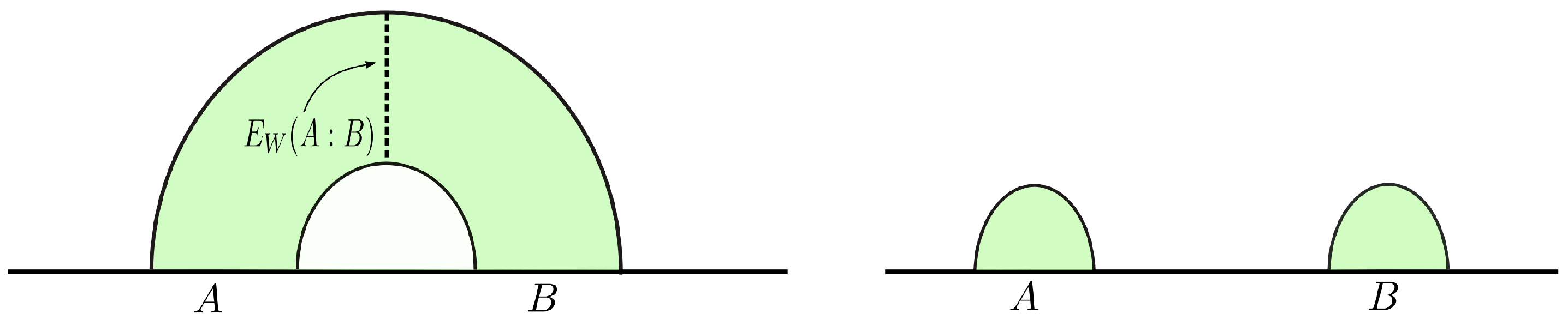
We begin this section by reviewing the construction for the bulk entanglement wedge cross section (EWCS) in AdS/CFT described in [43,44]. To this end, spatial subsystems A and B need to be considered in a CFTd dual to static bulk AdSd+1 geometry. Let be a constant time slice in the bulk and be an RT surface for the subsystem . Then, the codimension-one spatial region in bounded by is described as the entanglement wedge for subsystems A and B. Finally, we consider the minimal area surface which terminates on the boundary of the entanglement wedge, dividing the total entanglement wedge into two parts, as illustrated in Figure 1.
The entanglement wedge cross section (EWCS), denoted by , may then be defined as5
where is the Newton constant. The reduced density matrix is dual to the corresponding entanglement wedge [38,39,40]. Note that the entanglement wedge includes the bulk region, which is defined as the domain of dependence for the space-like homology surface bounded by subsystem A and its RT surface . Some of the properties of the EWCS are listed below [43,44].
- For a pure state , is equal to the entanglement entropy:
- For a mixed state , is bounded above by the entanglement entropy:
- For a mixed state , is bounded below by half the mutual information:
- is monotonic, i.e., it never increases upon discarding a subsystem:
- For a tripartite system, has the following bound:
- In a bipartite state that saturates the Araki–Lieb inequality, , we have .
- For a tripartite pure state, the is polygamous:
Note that these properties conform to the properties of the entanglement of purification (EoP) described in quantum information theory [64].
3.1. Computation of the EWCS
We now proceed to review the computation of the EWCS in the AdS3/CFT2 scenario. For this purpose, a configuration of two subsystems A and B at zero temperature needs to be considered in the dual CFT2 vacuum. These subsystems are described by spatial intervals and with lengths and , respectively, and are separated by distance d. The bulk dual for this case is a pure AdS3 geometry in Poincaré coordinates whose metric on a constant time slice is given by
where we have set the AdS3 radius . When the mutual information , the entanglement wedge remains connected; otherwise, it is disconnected. The EWCS for this configuration may be expressed as [43]
where the conformal cross ratio z is given by
Note that Equation (28) may be rewritten in the following form [35,65]:
where the cross ratio
is related to z through .
For a finite temperature state in a CFT2 defined on an infinite line, the bulk dual is a planar BTZ black hole (black string) whose metric is given as
where the event horizon is located at and is related to the inverse temperature as . The EWCS corresponding to the intervals and in a dual CFT2 is given as follows [43]:
with given as
3.1.1. EWCS for Two Disjoint Intervals
For this configuration, we will only describe the scenario where the two disjoint intervals are in proximity, which corresponds to the regime following [10,12]. It was shown there that the entanglement negativity obtained through a replica technique in a CFT2 was non-universal, and a dominant universal form could be obtained only for the above proximity regime in the large central charge limit. Note that, as explained in [10,12], the regime involves .6 In this regime, the EWCS for the two disjoint intervals in proximity is then obtained from Equation (30) as follows:
The EWCS for two disjoint intervals in proximity at zero temperature in a dual CFT2 may be derived by substituting Equation (31) into Equation (35) as follows:
For the intervals A and B in a finite size system of length L at zero temperature, the EWCS may be obtained via the conformal map from the plane to cylinder from Equation (35) as
The EWCS for two disjoint intervals in proximity at a finite temperature may be obtained from Equation (35) by employing the conformal transformation from the plane to the cylinder. It is then given by
3.1.2. EWCS for Two Adjacent Intervals
The mixed state configuration of two adjacent intervals may be constructed from the corresponding disjoint setup by taking the adjacent limit , where is the UV cutoff of the CFT2 in the boundary. The EWCS for this configuration may now be obtained from Equation (36) as follows:
By taking the adjacent limit in Equation (37), the EWCS for two adjacent intervals in a finite size system of length L may expressed as
The EWCS for two adjacent intervals at a finite temperature may be computed from Equation (38) by taking the adjacent limit as follows:
3.1.3. EWCS for a Single Interval
The EWCS for a pure state configuration of a single interval A of length l at zero temperature may be obtained from the property of the EWCS for a pure state, as described in Equation (21). It is given as
Similarly, the EWCS for a pure state configuration of a single interval A in a finite size system of length L may be computed using Equation (21) and given by
Subsequently, the authors in [43] proposed the EWCS for a mixed state configuration of a single interval A of length l at finite temperature as the minimum of two possible candidates, as expressed below:
The EWCS construction for this configuration will be described in detail in Section 4.3.3.
4. HEN from EWCS in AdS3/CFT2
In this section, we describe the construction in [35,37], which proposed the entanglement wedge cross section as the holographic dual of entanglement negativity. The authors in [43,44] had demonstrated that the EWCS was dual to the entanglement of purification (EoP) and followed all the properties of the EoP in quantum in formation theory [64]. Motivated by these developments and results from quantum error correcting codes, the authors in [35,37] conjectured that the EWCS backreacted by a bulk cosmic brane for the conical defect geometry is also dual to the entanglement negativity for configurations involving spherical entangling surfaces. The holographic entanglement negativity for the corresponding dual CFTs was then expressed in terms of the bulk EWCS as follows [35,37]:
where is the same dimension-dependent constant described in Section 2.1. The above conjecture was substantiated more concisely for holographic CFTs as [37]
where is a correlation measure termed as the reflected entropy and is the Rényi reflected entropy of order half. In the next few subsections, we briefly review the computation of the holographic entanglement negativity from the EWCS for various bipartite states described by two disjoint intervals, two adjacent intervals, and a single interval in the context of the AdS3/CFT2 scenario.
4.1. Negativity for Two Disjoint Intervals
4.1.1. Zero Temperature
The computation of the entanglement negativity for two disjoint intervals involves the four-point twist correlator whose explicit form contains an arbitrary non-universal function of the cross ratio and depends on the full operator content of the corresponding CFT2. Using Zamolodchikov recursion relations, the authors in [37] have numerically shown that the entanglement negativity for disjoint intervals is proportional to the EWCS. However, a recent development indicates the presence of an extra additive constant in the EWCS for two disjoint intervals in a CFT2, which may be determined through careful bulk computation [60]. As described earlier in Section 3.1.1, the entanglement negativity for two disjoint intervals in a CFT2 is non-universal for general values of the cross ratio x and a universal divergent behavior in the large central charge limit may be obtained for the regime , where the intervals are in proximity ().7 For this regime on using Equations (35) and (45), the holographic entanglement negativity for the mixed state of two disjoint intervals in proximity at zero temperature may be expressed as
where , are lengths of the intervals, and d is the length of the separation between intervals A and B. Note that the above result is cutoff-independent. The above result matches with the corresponding CFT2 replica result [9,10,12] obtained with the monodromy technique for the t channel in the regime modulo the second constant term. As discussed in Section 1, the constant second term in Equation (47) arises from the Markov gap.8 However, the result of holographic entanglement negativity for the two disjoint intervals obtained in [32] matches exactly with the corresponding field theory replica technique results. This illustrates the equivalence of the two holographic proposals for the entanglement negativity expressed in Equations (17) and (45) up to an additive constant.
4.1.2. Finite Size
The holographic entanglement negativity for the configuration of two disjoint intervals in a finite size CFT2 may be obtained using Equations (37) and (45) as
Note again that the result in Equation (48) is cutoff-independent. We observe again that apart from the constant term, the holographic entanglement negativity for two disjoint intervals in Equation (48) matches with the corresponding result from an earlier alternative proposal described in Equation (17) [32], demonstrating their equivalence.
4.1.3. Finite Temperature
For the mixed state configuration of two disjoint intervals at a finite temperature, the holographic entanglement negativity may be computed using Equations (38) and (45) as
Note that the expression in Equation (49) is once again cutoff-independent. The above equation matches with the entanglement negativity obtained by the field theory replica technique in CFT2s [10], modulo the additive constant in the large central charge limit. Once again, we observe that the holographic entanglement negativity in Equation (49) matches with that obtained from the alternative proposal described in Equation (17) [32] modulo the constant term, establishing their equivalence.
4.2. Negativity for Two Adjacent Intervals
4.2.1. Zero Temperature
The holographic entanglement negativity for the bipartite mixed state configuration described by two adjacent intervals at zero temperature in a CFT2 may be obtained from the backreacted EWCS using Equations (39) and (45) as follows:
where is the UV cutoff. We observe that the above result matches with the entanglement negativity obtained by the field theory replica technique in the large central charge limit [10] modulo the constant term related to the holographic Markov gap (see Appendix C). Note, however, that the holographic entanglement negativity for this mixed state configuration obtained through the alternate conjecture involving an algebraic sum of lengths of bulk geodesics in [30] matches exactly with the field theory results in the large c limit. This demonstrates the equivalence of the two holographic proposals for the entanglement negativity modulo the constant from the Markov gap.
4.2.2. Finite Size
The holographic entanglement negativity for the configuration of two adjacent intervals for a finite size CFT2 may be obtained using Equations (40) and (45) as
where is the UV cutoff. The above result also matches with the corresponding replica technique results [10] in the large central charge limit up to the Markov gap constant. Note that the above result in Equation (51) modulo the constant may also be obtained using the alternative proposal described in Equation (18) [30] which involves an algebraic sum of lengths of the bulk geodesics homologous to appropriate combinations of the intervals and illustrates their equivalence.
4.2.3. Finite Temperature
The EWCS for two adjacent intervals at a finite temperature may be computed from Equation (33) by taking the adjacent limit . Now, using Equation (45), the holographic entanglement negativity for the finite temperature mixed state configuration of two adjacent intervals in a CFT2 may be expressed as
where is the UV cutoff. As discussed earlier, the constant second term in the above equation may be related to the holographic Markov gap. The first term in Equation (52) matches with the corresponding result for holographic entanglement negativity in [30] using the alternate construction given in Equation (18) and the CFT2 replica technique result [10] in the large central charge limit. This once again demonstrates the equivalence of the two holographic entanglement negativity proposals modulo the Markov gap constant.
4.3. Negativity for a Single Interval
In this section, we consider the bipartite configuration of a single interval in a dual CFT2. To this end, the system , which includes the interval A of length l, with the rest of the system denoted as B, needs to be considered.
4.3.1. Zero Temperature
The holographic entanglement negativity for the pure state of a single interval A in a CFT2 at zero temperature may be obtained by considering the property of the EWCS described in Equation (21). Utilizing the holographic prescription from Equation (45) and the expression for the corresponding EWCS in Equation (42), the entanglement negativity for this pure state is given as
The above result matches exactly with the corresponding CFT2 replica technique result, as described in [9,10], in the large central charge limit. Interestingly, here, we observe the absence of any contribution related to the holographic Markov gap as the configuration of a single interval in zero temperature CFT2 is in a pure state. Thus, the holographic entanglement negativity in Equation (53) matches with that obtained from the alternative proposal in Equation (19) [26], once again illustrating their equivalence.
4.3.2. Finite Size
The holographic entanglement negativity for the pure state configuration of a single interval in a finite size system may be computed using Equations (43) and (45) as follows:
Note that the above result may also be obtained using the alternative holographic proposal, as described in Equation (19).
4.3.3. Finite Temperature
We begin with a brief review of the entanglement wedge construction in the context of a single interval in a CFT2 at a finite temperature, dual to a bulk planar BTZ black hole, as described in [43]. The authors in [43] considered the bipartition (Figure 2) comprising a single interval (of length l), denoted by A, with the rest of the system denoted by B. Note that in [43], , the minimal cross section of the entanglement wedge for the intervals A and B, has two possible candidates. The first one, denoted by , is the union of the two dotted lines depicted in Figure 2, while the other one, , is given by the RT surface . Then, the EWCS is given as [43]
where is the UV cutoff and is the inverse temperature.
Using the result of Equation (56), the authors in [35,37] described the holographic entanglement negativity of the single interval in a CFT2 at a finite temperature as
The authors substantiated their results utilizing the monodromy technique to extract the dominant contribution in the s and t channels for the relevant four-point twist correlator. However, the above results do not exactly reproduce the corresponding replica technique results for the mixed state configuration in question described in [11] except in the low- and high-temperature limits. Specifically, the subtracted thermal entropy term is missing from the holographic entanglement negativity and this issue requires further analysis. In Section 5, we will carefully investigate the above issue for the computation of the holographic entanglement negativity from the EWCS in [35,37] for the configuration in question.
5. Issue with the Thermal Entropy Term
Calabrese, Cardy, and Tonni in a significant communication [11] computed the entanglement negativity of a single interval (of length l) for a CFT2 at a finite temperature, which is given by
where is the UV cutoff. Here, f is an arbitrary function and is a constant, which are non-universal and depend on the full operator content of the theory.
Comparing Equation (57) with Equation (58), we note that the holographic entanglement negativity, as computed from Equation (45), does not match exactly9 with the corresponding replica technique result reported in [11], in the large central charge limit. Specifically, the subtracted thermal entropy term in the large c replica technique result is missing in the expression for the holographic entanglement negativity of a single interval at a finite temperature described in [35,37]. One may further observe that the entanglement negativity in Equation (58) reduces to that in Equation (57) only in the specific limits of low temperature () and high temperature (). In the next subsection, we briefly describe the monodromy analysis of the four-point twist correlator relevant for this configuration towards a resolution of the above issue with the subtracted thermal entropy term for the entanglement negativity.
5.1. Large Central Charge Limit
We begin by reviewing the results obtained through the monodromy technique employed in [37] to compute the entanglement negativity of a single interval, as given in Equation (57). To this end, two auxiliary intervals and on either side of the single interval (see [11] for details) need to be considered. The rest of the system is denoted by . Finally, we implement the bipartite limit through to arrive at the required configuration for the single interval A and the rest of the system . The entanglement negativity of a single interval at zero temperature in a CFT2 may then be described by the following four-point twist correlator on the complex plane [11]
Through a suitable conformal transformation (see [32] for a detailed review), Equation (59) may be recast as [37]
For a CFT2 at a finite temperature , the entanglement negativity for a single interval may be computed from Equation (59) or Equation (60) through the conformal transformation from the complex plane to the cylinder. The entanglement negativity for a single interval in a thermal CFT2 may then be obtained as follows [11,37]:
where the cross ratio x is specified by .
In the large central charge limit, the four-point twist correlator in Equation (61) may be expressed in terms of a dominant single conformal block in the s and t channels depending on the cross ratio x, as described in [29].
For the s channel (described by ), the authors in [37] have computed the four point function on the complex plane as
Utilizing the above four-point twist correlator, the entanglement negativity may be computed from Equation (61) as10
For the t channel (given by ), the authors in [37] have obtained the following four-point function:
from which the entanglement negativity may be obtained Equation (61):
We note that the four-point functions on the complex plane given in Equations (62) and (64), utilized to compute the entanglement negativity for both the channels, match those obtained in [29]. We further observe that the monodromy technique employed in [26,29] and the monodromy method utilized by the authors in [37] all produce identical large central charge limits for the four-point function.
However, we would like to emphasize here that the authors in [37], motivated by the large c computations for the entanglement entropy in [7,8], assumed that the s and t channel results are valid beyond their usual regimes and , that is, for and , respectively. In other words, their computation involves an assumption that there is a phase transition for the large central charge limit for the entanglement negativity of a single interval at . Although this is true for the entanglement entropy [7,8], for this specific case of the entanglement negativity for a single interval, this assumption is not valid, as the required four-point twist correlator is obtained from a specific channel for the corresponding six-point correlator, as described in [29]. The above conclusion is also supported by an alternate EWCS construction for this configuration proposed in Section 5.2 to resolve the issue with the missing thermal term for the holographic entanglement negativity in [35,37].
5.2. Alternate EWCS Construction
In this subsection, we propose an alternative construction to that described in [43] for the mixed state configuration of a single interval at a finite temperature in AdS3/CFT2. To this end, we consider the following properties [refer to Equation (26)] of the EWCS for tripartite pure state configurations comprising subsystems A, B, and C (see [43,44] for a review):
where is the mutual information between A and B. For two adjacent intervals A and B at a finite temperature in a CFT2 dual to a bulk planar BTZ black hole, the EWCS may be explicitly computed through the adjacent limit in the corresponding disjoint interval result derived in [43]. The holographic mutual information for these adjacent intervals may also be explicitly calculated from the corresponding entanglement entropies. Comparing these results, we obtain the following relation for this specific configuration:
Substituting the result described in Equation (68) into Equation (67) and comparing them with Equation (66), we arrive at the following equality for the bulk BTZ black hole configuration:
where B and C are adjacent to A.
Following the construction in [11], we now consider a tripartition (see Figure 3) consisting of interval A of length l, with two auxiliary intervals and , each of length L, on either side of A where . Next, we implement the bipartite limit to recover the original configuration with a single interval A and the rest of the system given by . Note that in the bipartite limit, describes the full system, which is in a pure state and obeys Equation (69). Thus, for this configuration (in the bipartite limit),
Computing the right-hand side of Equation (70), we obtain the EWCS for the bipartition involving the interval A and the rest of the system as follows:
The holographic entanglement negativity for the mixed state configuration of a single interval A in a CFT2 at a finite temperature dual to the bulk planar BTZ black hole may now be obtained by utilizing Equations (45) and (71) as follows:
The above expression matches exactly with the corresponding field theory replica technique result for the entanglement negativity described in Equation (58) in the large central charge limit up to a constant related to the Markov gap. Interestingly, the result for the holographic entanglement negativity for this mixed state configuration utilizing the alternate holographic construction involving the algebraic sum of bulk geodesics as reported in [26] matches exactly with the corresponding field theory replica technique results in the large c limit without the constant. This once again indicates the equivalence of the two proposals up to a constant.
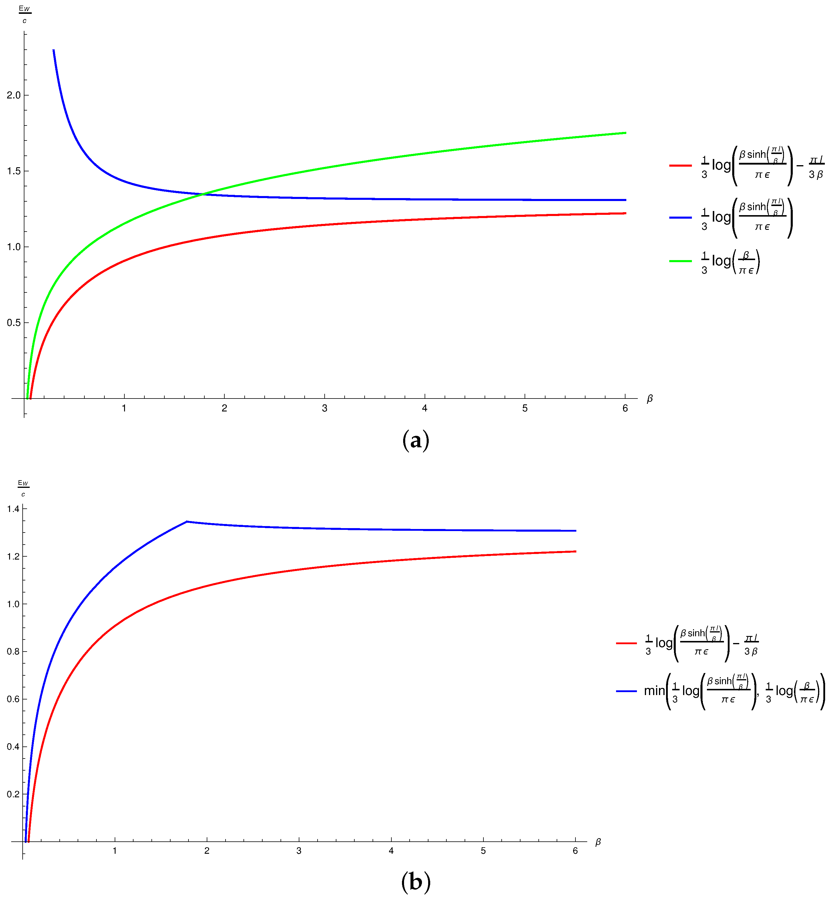
In Figure 4, we have plotted the possible candidates for the EWCS as a function of the inverse temperature to compare our construction with that described in [43] for this configuration. In Figure 4a, the two possible candidates (green and blue curves) for the EWCS described in Equation (56) have been compared with our expression given in Equation (71) without the third term (red curve). In Figure 4b, the proposed EWCS (blue curve), as prescribed in [43], given in Equation (56), has been plotted along with the EWCS modulo the constant (red curve) obtained by utilizing our alternative proposal, as described in Equation (71). It is interesting to note that our proposed EWCS always remains strictly less than that advanced in [43] for the range of used in the plot. This conclusively singles out our construction for the EWCS over the other proposal as the correct minimal EWCS, which also reproduces the replica technique result described in [11], in the large c limit. We also observe that Equations (56) and (71) asymptotically approaches each other in the limits of high () and low () temperatures. Naturally, this resolves the issue with the holographic entanglement negativity for this configuration and restores the missing thermal entropy term.
6. Discussions and Conclusions
To summarize, we have established the equivalence modulo the Markov gap constant of two different proposals in the literature for the holographic entanglement negativity of bipartite states in the context of the AdS3/CFT2 correspondence. The first proposal described in [26,30,32] involved an algebraic sum of the lengths of bulk geodesics homologous to certain combinations of subsystems, and the second one reported in [35,37] was based on the EWCS backreacted by a cosmic brane for the conical defect of the replicated bulk geometry in a gravitational path integral.
In this connection, we have analyzed and compared the results for the holographic entanglement negativity following from the above two proposals for various bipartite state configurations described by two disjoint intervals, two adjacent intervals, and a single interval in dual CFT2s. We observe that the results obtained from these two proposals match each other up to certain constants which arise from the Markov gap for the EWCS, establishing their equivalence.
In this context, we have investigated a critical issue with the proposal involving the backreacted EWCS for the holographic entanglement negativity of a single interval in a finite temperature CFT2 dual to a bulk planar BTZ black hole. Specifically, the holographic entanglement negativity obtained for the above configuration from the backreacted EWCS excluded a subtracted thermal entropy term in the corresponding field theory replica technique result at large c. In this article, we have resolved this significant issue by proposing an alternative construction for the EWCS of this configuration, which is actually the minimal one. Our construction involved the introduction of two large auxiliary intervals adjacent to the single interval in question. Subsequently, a bipartite limit for this configuration was implemented through the consideration of the auxiliary intervals to be infinite and constitute the rest of the system. To this end, we utilized certain polygamy properties to obtain the correct bulk EWCS for the single interval in a holographic CFT2. Interestingly, our results following from the above construction reproduced the excluded thermal term and matched the field theory replica technique result exactly in the large central charge limit in the literature. Naturally, the holographic entanglement negativity proposal involving the backreacted EWCS requires substantiation from explicit higher-dimensional examples for generic AdSd+1/CFTd scenarios. However, the difficulties for the computation of the EWCS for higher dimensions are well known. We hope to address some of these issues in the near future.
Author Contributions
Conceptualization, J.K.B., V.M., H.P., B.P. and G.S.; methodology, J.K.B., V.M., H.P., B.P. and G.S.; formal analysis, J.K.B., V.M., H.P., B.P. and G.S.; writing—original draft preparation, J.K.B., V.M., H.P., B.P. and G.S.; writing—review and editing, J.K.B., V.M., H.P., B.P. and G.S. All authors have read and agreed to the published version of the manuscript.
Funding
The work of J.K.B. is supported by the National Science and Technology Council of Taiwan with the grant 112-2636-M-110-006. The work of V.M. is supported by the NRF grant funded by the Korea government (MSIT) (No. 2022R1A2C1003182) and by the Brain Pool program funded by the Ministry of Science and ICT through the National Research Foundation of Korea (RS-2023-00261799). The work of H.P. is supported by the NCTS, Taiwan. The work of G.S. is partially supported by the Jag Mohan Garg Chair Professor position at the Indian Institute of Technology, Kanpur.
Data Availability Statement
No new data were created or analyzed in this study. Data sharing is not applicable to this article.
Acknowledgments
We acknowledge Jonah Kudler-Flam, Yuya Kusuki, and Shinsei Ryu for their communication, which led to this work. We also thank Saikat Ghosh, Debarshi Basu, and Vinayak Raj for crucial discussions.
Conflicts of Interest
The authors declare no conflicts of interest.
Appendix A. Entanglement Negativity of Two Disjoint Intervals
In this appendix, following [9,10,12], we describe the derivation of the entanglement negativity for two disjoint intervals in a CFT2 through a replica technique in the large central charge limit. The entanglement negativity for this case is described by a four-point twist field correlator involving a non-universal function of the cross ratio x, which depends on the full operator content of the theory. As described in [10], it is not possible to evaluate this non-universal function analytically for general values of the cross ratio x. However, it may be approximated in the large central charge limit for the regimes characterized by and when the intervals are far away and in proximity, respectively.11 These two regimes are described in the s and t channel approximations for the four-point correlator involving the fusion of distinct pairs of the twist fields.12 As shown in [10], the non-universal function vanishes non-perturbatively in the regime for the s channel at a large c. On the other hand, for the regime for the t channel, the four-point twist correlator admits the following conformal block expansion, as described in [12]
where the summation is taken over by all the primary operators with conformal dimensions , and represent the conformal dimensions of the twist operators on the left-hand side of Equation (A1). Note that apart from some particular values of the parameters, it is not possible to analytically derive . In the semi-classical approximation characterized by with fixed, the conformal block exponentiates as follows [66,67]:
The function f in Equation (A2) may be computed through the monodromy properties of the solutions of a second-order differential equation.13 In the semi-classical regime, the dominant contribution was shown to arise from the conformal block for the intermediate operator with the lowest conformal dimension in the exchange channel.
For two disjoint intervals in proximity ( in the t channel), the relevant intermediate operator with the lowest conformal dimension is [12]. Hence, the conformal block with the conformal dimension provides the dominant contribution to the correlator in Equation (A1). Utilizing Equation (A2), the correlator in Equation (A1) may then be expressed at a large c as14
and the function f in this case is determined from a monodromy analysis to be [12]
which describes a universal divergent behavior as x approaches 1. The four-point twist correlator in Equation (A3) may then be expressed at a large c as
The entanglement negativity for two disjoint intervals in proximity () may now be computed from Equation (A5) as follows [12]:
where we have utilized the relation . The solution for a general value of the cross ratio x is not amenable to analytic methods; however, a consistent numerical analysis has been described in [12], although several open issues remain.15
We note here that in [7], the entanglement entropy for two disjoint intervals at a large c limit was shown to display a phase transition from its s channel value to its t channel value at . Interestingly, in [12], a similar phase transition was demonstrated through the numerical analysis described above for the corresponding entanglement negativity at a large c, from its s channel value of zero to its t channel value given by Equation (A6), although the corresponding critical value of x for the transition could not be established. However, due to the existence of a correspondence between the classical geometries dual to the Rényi entanglement entropy and the Rényi entanglement negativity, as shown in [13], it could be expected that this phase transition also occurs at .
Appendix B. HEN and Replica Symmetry Breaking Saddle
In this appendix, we review a plausible derivation of the holographic proposal involving the algebraic sum of the areas of backreacting cosmic branes, as described in [61], which utilized the replica symmetry breaking saddle reported in [68]. As discussed in [9,10], a Rényi generalization for the entanglement negativity may be defined as follows:
where denotes the replicated manifold for the entanglement negativity where different copies of the subsystem A are glued cyclically and the copies of B are glued anti-cyclically, denotes the original manifold, and Z denotes their respective path integrals. The entanglement negativity is then given by the analytic continuation of even Rényi negativities () defined above to as
In holography, this implies that the entanglement negativity at the leading order is related to the corresponding bulk gravitational on-shell actions in the saddle point approximation, as follows:
Note that the odd analytic continuation of Equation (A7) to does not lead to entanglement negativity but simply gives back the trace condition. Quite interestingly, the authors in [68] demonstrated that the replica symmetric gravitational saddle is the same for even and odd k and leads to a vanishing result for the entanglement negativity:
The authors showed that, remarkably, the dominant saddle corresponding to the entanglement negativity breaks the replica symmetry in the bulk spacetime. The holographic construction of the replica non-symmetric saddle is as follows: Consider copies of the bulk manifold which are cut along three non-overlapping codimension-one homology hypersurfaces , and that obey the homology condition , where is the codimension-two hypersurface homologous to X. Now, different homology hypersurfaces are glued as follows:
- : odd-numbered copies of the bulk manifold are glued cyclically, whereas the even ones are glued to themselves;
- : even-numbered copies of bulk manifold are glued anti-cyclically, whereas the odd ones are glued to themselves;
- : all the copies are glued pairwise.
Observe that the above construction respects the replica symmetry in the boundary; however, it is explicitly broken from in the bulk. This led the authors in [68] to consider the quotient of the original manifold:
This quotienting has the following effect on the corresponding gravitational on-shell actions:
where corresponds to the on-shell bulk action for the alternative construction of the quotiented bulk manifold with conical deficits along the codimension-two surfaces and (subscripts 1 and 2 simply indicate in which copy the codimension-two surface is located), and having as its asymptotic boundary. Substituting the above equation in Equation (A9) and utilizing the result obtained in Equation (A7) lead to the following expression for the Rényi entanglement negativity:
Following the above result, in [61], the authors utilized a result for the bulk action away from given in [69,70] to arrive at the following expression for the on-shell action:
Implementing the limit in the above equation, inserting it into Equation (A13), and finally substituting the result obtained into Equation (A8) lead to the following expression for the holographic entanglement negativity:
where in the last line, denotes the holographic Rényi mutual information of order half for the bipartite system . Note that in order to arrive at Equation (A13), the authors in [68] assumed that the subsystems A, B, and are together in a tripartite pure state. Upon imposing this assumption in the holographic constructions for the entanglement negativity of a single interval, two adjacent intervals, and two disjoint intervals [26,30,32], the authors in [61] demonstrated that they all reduce to the above expression.
Appendix C. HEN and Markov Gap
In this appendix, we describe the crucial role of the holographic Markov gap to the holographic entanglement negativity proposals described in [28,32,35,37]. Before we discuss the relation of the Markov gap to the holographic entanglement negativity, let us briefly review the definition of the reflected entropy described in [36] and the holographic Markov gap, as explained in [60]. To this end, consider a bipartite mixed state . There exists a canonical purification in the doubled Hilbert spaces . The von Neumann entropy of the bipartite state , which is obtained from the state by tracing over the degrees of freedom of , is known as the reflected entropy [36]:
Now, consider the action of a quantum channel which acts on the bipartite mixed state to produce a tripartite state :
The Markov recovery process refers to reproducing the quantum state , whose reduction led to the bipartite mixed state through the operation of the above quantum channel , which acts on subsystem B alone. If , the Markov recovery process is said to be perfect and the state is said to be a quantum Markov chain for the ordering . Furthermore, it has been shown through quantum information techniques that this happens when the conditional mutual information vanishes [71]. This result was further refined in [72], where the authors demonstrated that there exists a bound expressed as follows:
where is the quantum fidelity which is in unity when and zero when the two density matrices have support on orthogonal subspaces. This led the authors to examine the above bound for the Markov recovery process of the reduced density matrix that occurs in the canonical purification . This immediately implies the following constraint on the conditional mutual information because of the above inequality:
where in the last line, the conditional mutual information is simply re-expressed in terms of the reflected entropy and the mutual information which the authors in [60] termed as the Markov gap. Furthermore, in the context of AdS3/CFT2, the authors demonstrated that the above bound may be expressed geometrically as follows:
where refers to the AdS radius and the # of boundaries of EWCS denotes the number of end points of EWCS in the bulk AdS3 geometry (boundaries at asymptotic infinity are not considered as they are infinitely far away).
In order to understand the connection of the holographic Markov gap to the holographic entanglement negativity, consider an alternative proposal for it developed in [35,37]. As explained in detail in Section 4, the authors in [35] proposed that the holographic entanglement negativity is given by the area of the backreacting EWCS. This proposal was further refined in [37], where the authors related it to the Rényi reflected entropy of order half as follows:
where the second equality is valid when and share a spherical entangling surface in higher dimensions or when is a continuous interval in AdS3/CFT2 [37]. We have denoted the entanglement negativity computed from this proposal as to distinguish it from that obtained through the proposal involving the mutual information of order half in Equation (A16). Consider now the difference between the holographic entanglement negativity computed using these two proposals:
As discussed in Section 2.1, for subsystems with spherical entangling surfaces and in AdS3/CFT2, the Rényi entropies of order half of A, B, and are proportional to their corresponding von Neumann entropies, as given by Equation (A8), and hence, the above equation reduces to
where in order to arrive at the last line of the above equation, we have utilized the inequality given in Equation (A23) and . Thus, the difference between the entanglement negativities computed from the two proposals is proportional to the Markov gap, which is non-vanishing in a holographic CFT2, as described by the above equation.
| 1 | Several other measures to characterize mixed state entanglement have also been proposed in quantum information theory. However, most of these involve optimization over LOCC protocols and are not directly computable. |
| 2 | The authors in [63] utilized a conformal map from a hyperbolic cylinder to the causal evolution of a subregion enclosed by a spherical entangling surface in flat space. This in turn implies that the entanglement entropy of a spherical region in a CFT on a flat Minkowski space is given by an integral of thermal entropy of a CFT on a hyperbolic cylinder. In the context of AdS/CFT correspondence, this translates to computing the horizon entropy of a certain topological black hole by the well-known Wald formula. |
| 3 | The trace norm for an arbitrary hermitian matrix M is given by . |
| 4 | For details of this proof, refer to [61]. |
| 5 | Note that sometimes the minimal surface itself is referred to as the entanglement wedge cross section. The meaning is usually clear from the context. |
| 6 | In the literature, the regime has been loosely stated as the limit . However, such a limit will force the EWCS to be divergent and implies setting , which is not possible as , where is the UV cutoff in the CFT2. |
| 7 | A brief review of the determination of the entanglement negativity for disjoint intervals from a field theory replica technique approach, as described in [10,12], has been provided in Appendix A. |
| 8 | The holographic Markov gap between the reflected entropy and the mutual information is briefly described in Appendix C. For details, see [60]. |
| 9 | In [43], the authors have indicated that for a single interval at a finite temperature with a length , the extensive contribution is missing in the expression for the EWCS, as described in Equation (56). |
| 10 | Note that we have omitted a Markov gap term on the right-hand side of Equation (63). |
| 11 | Note that, as explained in [10], the proximity regime does not involve setting the separation d between the intervals equal to the UV cutoff in the CFT2 with a clear hierarchy . In particular, it is not equivalent to the limit , which will force . |
| 12 | Note that the s and t channels are characterized by and respectively. |
| 13 | Refer to [12] for details of this monodromy technique and related computations. |
| 14 | |
| 15 | Note that in [35], the corresponding bulk EWCS has been numerically evaluated assuming an ad hoc conformal block-like expansion. As the EWCS is a bulk geometrical quantity, it is not clear from their analysis why such an expansion should be valid. |
References
- Vidal, G.; Werner, R.F. Computable measure of entanglement. Phys. Rev. A 2002, 65, 032314. [Google Scholar] [CrossRef]
- Plenio, M.B. Logarithmic Negativity: A Full Entanglement Monotone That is not Convex. Phys. Rev. Lett. 2005, 95, 090503. [Google Scholar] [CrossRef]
- Calabrese, P.; Cardy, J.L. Entanglement entropy and quantum field theory. J. Stat. Mech. 2004, 0406, P06002. [Google Scholar] [CrossRef]
- Calabrese, P.; Cardy, J. Entanglement entropy and conformal field theory. J. Phys. A 2009, 42, 504005. [Google Scholar] [CrossRef]
- Calabrese, P.; Cardy, J.; Tonni, E. Entanglement entropy of two disjoint intervals in conformal field theory. J. Stat. Mech. 2009, 0911, P11001. [Google Scholar] [CrossRef]
- Calabrese, P.; Cardy, J.; Tonni, E. Entanglement entropy of two disjoint intervals in conformal field theory II. J. Stat. Mech. 2011, 1101, P01021. [Google Scholar] [CrossRef]
- Hartman, T. Entanglement Entropy at Large Central Charge. arXiv 2013, arXiv:1303.6955. [Google Scholar]
- Headrick, M. Entanglement Renyi entropies in holographic theories. Phys. Rev. D 2010, 82, 126010. [Google Scholar] [CrossRef]
- Calabrese, P.; Cardy, J.; Tonni, E. Entanglement negativity in quantum field theory. Phys. Rev. Lett. 2012, 109, 130502. [Google Scholar] [CrossRef]
- Calabrese, P.; Cardy, J.; Tonni, E. Entanglement negativity in extended systems: A field theoretical approach. J. Stat. Mech. 2013, 1302, P02008. [Google Scholar] [CrossRef]
- Calabrese, P.; Cardy, J.; Tonni, E. Finite temperature entanglement negativity in conformal field theory. J. Phys. A 2015, 48, 015006. [Google Scholar] [CrossRef]
- Kulaxizi, M.; Parnachev, A.; Policastro, G. Conformal Blocks and Negativity at Large Central Charge. J. High Energy Phys. 2014, 09, 010. [Google Scholar] [CrossRef]
- Dong, X.; Maguire, S.; Maloney, A.; Maxfield, H. Phase transitions in 3D gravity and fractal dimension. J. High Energy Phys. 2018, 05, 080. [Google Scholar] [CrossRef]
- Ryu, S.; Takayanagi, T. Holographic derivation of entanglement entropy from AdS/CFT. Phys. Rev. Lett. 2006, 96, 181602. [Google Scholar] [CrossRef] [PubMed]
- Ryu, S.; Takayanagi, T. Aspects of Holographic Entanglement Entropy. J. High Energy Phys. 2006, 08, 045. [Google Scholar] [CrossRef]
- Nishioka, T.; Ryu, S.; Takayanagi, T. Holographic Entanglement Entropy: An Overview. J. Phys. A 2009, 42, 504008. [Google Scholar] [CrossRef]
- Rangamani, M.; Takayanagi, T. Holographic Entanglement Entropy. Lect. Notes Phys. 2017, 931, 1. [Google Scholar] [CrossRef]
- Nishioka, T. Entanglement entropy: Holography and renormalization group. Rev. Mod. Phys. 2018, 90, 035007. [Google Scholar] [CrossRef]
- Fursaev, D.V. Proof of the holographic formula for entanglement entropy. J. High Energy Phys. 2006, 09, 018. [Google Scholar] [CrossRef]
- Casini, H.; Huerta, M.; Myers, R.C. Towards a derivation of holographic entanglement entropy. J. High Energy Phys. 2011, 05, 036. [Google Scholar] [CrossRef]
- Faulkner, T. The Entanglement Renyi Entropies of Disjoint Intervals in AdS/CFT. arXiv 2013, arXiv:1303.7221. [Google Scholar]
- Lewkowycz, A.; Maldacena, J. Generalized gravitational entropy. J. High Energy Phys. 2013, 08, 090. [Google Scholar] [CrossRef]
- Hubeny, V.E.; Rangamani, M.; Takayanagi, T. A Covariant holographic entanglement entropy proposal. J. High Energy Phys. 2007, 07, 062. [Google Scholar] [CrossRef]
- Dong, X.; Lewkowycz, A.; Rangamani, M. Deriving covariant holographic entanglement. J. High Energy Phys. 2016, 11, 028. [Google Scholar] [CrossRef]
- Rangamani, M.; Rota, M. Comments on Entanglement Negativity in Holographic Field Theories. J. High Energy Phys. 2014, 10, 060. [Google Scholar] [CrossRef]
- Chaturvedi, P.; Malvimat, V.; Sengupta, G. Holographic Quantum Entanglement Negativity. J. High Energy Phys. 2018, 05, 172. [Google Scholar] [CrossRef]
- Chaturvedi, P.; Malvimat, V.; Sengupta, G. Covariant holographic entanglement negativity. Eur. Phys. J. C 2018, 78, 776. [Google Scholar] [CrossRef]
- Chaturvedi, P.; Malvimat, V.; Sengupta, G. Entanglement negativity, Holography and Black holes. Eur. Phys. J. C 2018, 78, 499. [Google Scholar] [CrossRef]
- Malvimat, V.; Sengupta, G. Entanglement negativity at large central charge. Phys. Rev. D 2021, 103, 106003. [Google Scholar] [CrossRef]
- Jain, P.; Malvimat, V.; Mondal, S.; Sengupta, G. Holographic entanglement negativity conjecture for adjacent intervals in AdS3/CFT2. Phys. Lett. B 2019, 793, 104. [Google Scholar] [CrossRef]
- Jain, P.; Malvimat, V.; Mondal, S.; Sengupta, G. Covariant holographic entanglement negativity for adjacent subsystems in AdS3 /CFT2. Nucl. Phys. B 2019, 945, 114683. [Google Scholar] [CrossRef]
- Malvimat, V.; Mondal, S.; Paul, B.; Sengupta, G. Holographic entanglement negativity for disjoint intervals in AdS3/CFT2. Eur. Phys. J. C 2019, 79, 191. [Google Scholar] [CrossRef]
- Malvimat, V.; Mondal, S.; Paul, B.; Sengupta, G. Covariant holographic entanglement negativity for disjoint intervals in AdS3/CFT2. Eur. Phys. J. C 2019, 79, 514. [Google Scholar] [CrossRef]
- Basak, J.K.; Parihar, H.; Paul, B.; Sengupta, G. Holographic entanglement negativity for disjoint subsystems in AdSd+1/CFTd. arXiv 2020, arXiv:2001.10534. [Google Scholar]
- Kudler-Flam, J.; Ryu, S. Entanglement negativity and minimal entanglement wedge cross sections in holographic theories. Phys. Rev. D 2019, 99, 106014. [Google Scholar] [CrossRef]
- Dutta, S.; Faulkner, T. A canonical purification for the entanglement wedge cross-section. J. High Energy Phys. 2021, 03, 178. [Google Scholar] [CrossRef]
- Kusuki, Y.; Kudler-Flam, J.; Ryu, S. Derivation of holographic negativity in AdS3/CFT2. Phys. Rev. Lett. 2019, 123, 131603. [Google Scholar] [CrossRef]
- Czech, B.; Karczmarek, J.L.; Nogueira, F.; Van Raamsdonk, M. The Gravity Dual of a Density Matrix. Class. Quant. Grav. 2012, 29, 155009. [Google Scholar] [CrossRef]
- Wall, A.C. Maximin Surfaces, and the Strong Subadditivity of the Covariant Holographic Entanglement Entropy. Class. Quant. Grav. 2014, 31, 225007. [Google Scholar] [CrossRef]
- Headrick, M.; Hubeny, V.E.; Lawrence, A.; Rangamani, M. Causality & holographic entanglement entropy. J. High Energy Phys. 2014, 12, 162. [Google Scholar] [CrossRef]
- Jafferis, D.L.; Suh, S.J. The Gravity Duals of Modular Hamiltonians. J. High Energy Phys. 2016, 09, 068. [Google Scholar] [CrossRef]
- Jafferis, D.L.; Lewkowycz, A.; Maldacena, J.; Suh, S.J. Relative entropy equals bulk relative entropy. J. High Energy Phys. 2016, 06, 004. [Google Scholar] [CrossRef]
- Takayanagi, T.; Umemoto, K. Entanglement of purification through holographic duality. Nat. Phys. 2018, 14, 573. [Google Scholar] [CrossRef]
- Nguyen, P.; Devakul, T.; Halbasch, M.G.; Zaletel, M.P.; Swingle, B. Entanglement of purification: From spin chains to holography. J. High Energy Phys. 2018, 01, 098. [Google Scholar] [CrossRef]
- Terhal, B.M.; Horodecki, M.; Leung, D.W.; DiVincenzo, D.P. The entanglement of purification. J. Math. Phys. 2002, 43, 4286. [Google Scholar] [CrossRef]
- Bhattacharyya, A.; Takayanagi, T.; Umemoto, K. Entanglement of Purification in Free Scalar Field Theories. J. High Energy Phys. 2018, 04, 132. [Google Scholar] [CrossRef]
- Bao, N.; Halpern, I.F. Holographic Inequalities and Entanglement of Purification. J. High Energy Phys. 2018, 03, 006. [Google Scholar] [CrossRef]
- Hirai, H.; Tamaoka, K.; Yokoya, T. Towards Entanglement of Purification for Conformal Field Theories. Prog. Theor. Exp. Phys. 2018, 2018, 063B03. [Google Scholar] [CrossRef]
- Espíndola, R.; Guijosa, A.; Pedraza, J.F. Entanglement Wedge Reconstruction and Entanglement of Purification. Eur. Phys. J. C 2018, 78, 646. [Google Scholar] [CrossRef]
- Umemoto, K.; Zhou, Y. Entanglement of Purification for Multipartite States and its Holographic Dual. J. High Energy Phys. 2018, 10, 152. [Google Scholar] [CrossRef]
- Bao, N.; Halpern, I.F. Conditional and Multipartite Entanglements of Purification and Holography. Phys. Rev. D 2019, 99, 046010. [Google Scholar] [CrossRef]
- Umemoto, K. Quantum and Classical Correlations Inside the Entanglement Wedge. Phys. Rev. D 2019, 100, 126021. [Google Scholar] [CrossRef]
- Guo, W.-Z. Entanglement of purification and disentanglement in CFTs. J. High Energy Phys. 2019, 09, 080. [Google Scholar] [CrossRef]
- Bao, N.; Chatwin-Davies, A.; Pollack, J.; Remmen, G.N. Towards a Bit Threads Derivation of Holographic Entanglement of Purification. J. High Energy Phys. 2019, 07, 152. [Google Scholar] [CrossRef]
- Harper, J.; Headrick, M. Bit threads and holographic entanglement of purification. J. High Energy Phys. 2019, 08, 101. [Google Scholar] [CrossRef]
- Tamaoka, K. Entanglement Wedge Cross Section from the Dual Density Matrix. Phys. Rev. Lett. 2019, 122, 141601. [Google Scholar] [CrossRef]
- Jeong, H.-S.; Kim, K.-Y.; Nishida, M. Reflected Entropy and Entanglement Wedge Cross Section with the First Order Correction. J. High Energy Phys. 2019, 12, 170. [Google Scholar] [CrossRef]
- Bao, N.; Cheng, N. Multipartite Reflected Entropy. J. High Energy Phys. 2019, 10, 102. [Google Scholar] [CrossRef]
- Chu, J.; Qi, R.; Zhou, Y. Generalizations of Reflected Entropy and the Holographic Dual. J. High Energy Phys. 2020, 03, 151. [Google Scholar] [CrossRef]
- Hayden, P.; Parrikar, O.; Sorce, J. The Markov gap for geometric reflected entropy. J. High Energy Phys. 2021, 10, 047. [Google Scholar] [CrossRef]
- Basak, J.K.; Basu, D.; Malvimat, V.; Parihar, H.; Sengupta, G. Islands for entanglement negativity. SciPost Phys. 2022, 12, 003. [Google Scholar] [CrossRef]
- Dong, X. The Gravity Dual of Renyi Entropy. Nat. Commun. 2016, 7, 12472. [Google Scholar] [CrossRef]
- Hung, L.-Y.; Myers, R.C.; Smolkin, M.; Yale, A. Holographic Calculations of Renyi Entropy. J. High Energy Phys. 2011, 12, 047. [Google Scholar] [CrossRef]
- Bagchi, S.; Pati, A.K. Monogamy, polygamy, and other properties of entanglement of purification. Phys. Rev. A 2015, 91, 042323. [Google Scholar] [CrossRef]
- Kudler-Flam, J.; Nozaki, M.; Ryu, S.; Tan, M.T. Quantum vs. classical information: Operator negativity as a probe of scrambling. J. High Energy Phys. 2020, 01, 031. [Google Scholar] [CrossRef]
- Belavin, A.A.; Polyakov, A.M.; Zamolodchikov, A.B. Infinite Conformal Symmetry in Two-Dimensional Quantum Field Theory. Nucl. Phys. B 1984, 241, 333. [Google Scholar] [CrossRef]
- Zamolodchikov, A.B. Conformal symmetry in two-dimensional space: Recursion representation of conformal block. Theor. Math. Phys. 1987, 73, 1088. [Google Scholar] [CrossRef]
- Dong, X.; Qi, X.-L.; Walter, M. Holographic entanglement negativity and replica symmetry breaking. J. High Energy Phys. 2021, 06, 024. [Google Scholar] [CrossRef]
- Nakaguchi, Y.; Nishioka, T. A holographic proof of Rényi entropic inequalities. J. High Energy Phys. 2016, 12, 129. [Google Scholar] [CrossRef]
- Kawabata, K.; Nishioka, T.; Okuyama, Y.; Watanabe, K. Replica wormholes and capacity of entanglement. J. High Energy Phys. 2021, 10, 227. [Google Scholar] [CrossRef]
- Petz, D. Sufficient subalgebras and the relative entropy of states of a von Neumann algebra. Commun. Math. Phys. 1986, 105, 123. [Google Scholar] [CrossRef]
- Fawzi, O.; Renner, R. Quantum Conditional Mutual Information and Approximate Markov Chains. Commun. Math. Phys. 2015, 340, 575. [Google Scholar] [CrossRef]
Figure 1.
(Left): The colored region represents the entanglement wedge for subsystem in Poincaré AdS3. The dotted line shows the entanglement wedge cross section. (Right): If A and B are sufficiently far away, the entanglement wedge becomes disconnected and .
Figure 1.
(Left): The colored region represents the entanglement wedge for subsystem in Poincaré AdS3. The dotted line shows the entanglement wedge cross section. (Right): If A and B are sufficiently far away, the entanglement wedge becomes disconnected and .

Figure 2.
EWCS for a single interval A (with rest of the system B) in a thermal CFT2 on the boundary, dual to a bulk planar BTZ black hole geometry.
Figure 2.
EWCS for a single interval A (with rest of the system B) in a thermal CFT2 on the boundary, dual to a bulk planar BTZ black hole geometry.
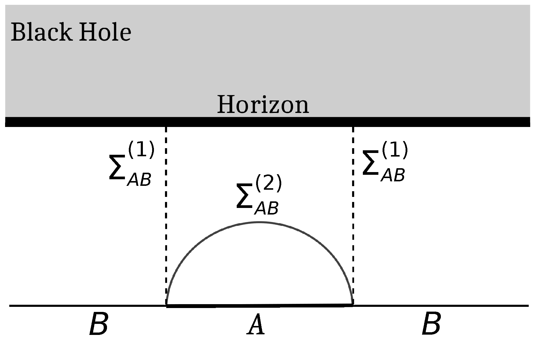
Figure 3.
Alternate computation of the EWCS (dotted lines) for a single interval A (with rest of the system B) in a finite temperature CFT2, dual to a planar bulk BTZ black hole geometry.
Figure 3.
Alternate computation of the EWCS (dotted lines) for a single interval A (with rest of the system B) in a finite temperature CFT2, dual to a planar bulk BTZ black hole geometry.
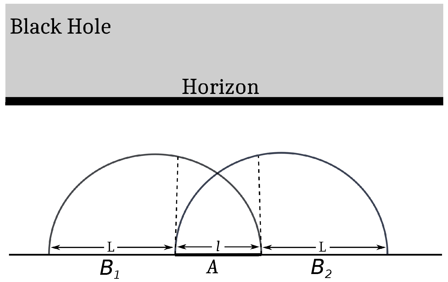
Figure 4.
Plots for different choices of EWCS against the inverse temperature for a single interval at a finite temperature. Here, and . (a) vs. plots for various candidates for EWCS. (b) vs. plots for EWCS utilizing the two different constructions.
Figure 4.
Plots for different choices of EWCS against the inverse temperature for a single interval at a finite temperature. Here, and . (a) vs. plots for various candidates for EWCS. (b) vs. plots for EWCS utilizing the two different constructions.
Disclaimer/Publisher’s Note: The statements, opinions and data contained in all publications are solely those of the individual author(s) and contributor(s) and not of MDPI and/or the editor(s). MDPI and/or the editor(s) disclaim responsibility for any injury to people or property resulting from any ideas, methods, instructions or products referred to in the content. |
© 2024 by the authors. Licensee MDPI, Basel, Switzerland. This article is an open access article distributed under the terms and conditions of the Creative Commons Attribution (CC BY) license (https://creativecommons.org/licenses/by/4.0/).
Share and Cite
MDPI and ACS Style
Basak, J.K.; Malvimat, V.; Parihar, H.; Paul, B.; Sengupta, G. On Minimal Entanglement Wedge Cross Section for Holographic Entanglement Negativity. Universe 2024, 10, 125. https://doi.org/10.3390/universe10030125
AMA Style
Basak JK, Malvimat V, Parihar H, Paul B, Sengupta G. On Minimal Entanglement Wedge Cross Section for Holographic Entanglement Negativity. Universe. 2024; 10(3):125. https://doi.org/10.3390/universe10030125
Chicago/Turabian StyleBasak, Jaydeep Kumar, Vinay Malvimat, Himanshu Parihar, Boudhayan Paul, and Gautam Sengupta. 2024. "On Minimal Entanglement Wedge Cross Section for Holographic Entanglement Negativity" Universe 10, no. 3: 125. https://doi.org/10.3390/universe10030125
Note that from the first issue of 2016, this journal uses article numbers instead of page numbers. See further details here.