Simple Lévy α-Stable Model Analysis of Elastic pp and $p\overline{p}$ Low-|t| Data from SPS to LHC Energies

Abstract

A simple Lévy $\alpha$-stable (SL) model is used to describe the data on elastic $pp$ and $p\overline{p}$ scattering at low-$\left|t\right|$ from SPS energies up to LHC energies. The SL model is demonstrated to describe the data with a strong non-exponential feature in a statistically acceptable manner. The energy dependence of the parameters of the model is determined and analyzed. The Lévy $\alpha$ parameter of the model has an energy-independent value of 1.959 ± 0.002 following from the strong non-exponential behavior of the data. We strengthen the conclusion that the discrepancy between TOTEM and ATLAS elastic $pp$ differential cross section measurements arises only in the normalization and not in the shape of the distribution of the data as a function of t. We find that the slope parameter has different values for $pp$ and $p\overline{p}$ elastic scattering at LHC energies. This may be the effect of the odderon exchange or the jump in the energy dependence of the slope parameter in the energy interval 3 GeV $\lesssim \sqrt{s}\lesssim$ 4 GeV.

1. Introduction

The physics of elastic proton–proton ($pp$) and proton–antiproton ($p\overline{p}$) scattering can be studied by measuring the differential cross section $d{\sigma }_{\mathrm{el}}/dt$ at a given center of mass (cm) energy $\sqrt{s}$ as a function of the squared four-momentum transfer t. The characteristic structure of the t-distribution of elastic $pp$ scattering was revealed in the 1970s by experiments performed with the ISR accelerator at CERN [1,2] in the energy range $23\mathrm{GeV}\lesssim \sqrt{s}\lesssim 63\mathrm{GeV}$. It was found that after the Coulomb-nuclear interference region at very small $\left|t\right|$ values, the $d{\sigma }_{\mathrm{el}}/dt$ is nearly exponentially decreasing in the range of $0.01{\mathrm{GeV}}^2\lesssim \left|t\right|\lesssim 1{\mathrm{GeV}}^2$ and has a characteristic diffractive minimum–maximum (dip-bump) structure in the domain $1{\mathrm{GeV}}^2\lesssim \left|t\right|\lesssim 2.5{\mathrm{GeV}}^2$. Beyond the bump, $\left|t\right|\gtrsim 3$ ${\mathrm{GeV}}^2$, the $d{\sigma }_{\mathrm{el}}/dt$ was found to be decreasing according to a power law ${\left|t\right|}^{-n}$ with $n\approx 8$ [3]. Measurements on $pp$ elastic scattering at LHC by TOTEM and ATLAS Collaborations at $\sqrt{s}=$ 2.76, 7, 8, and 13 TeV [4,5,6,7,8,9,10,11,12,13] confirm the structure of the t distribution of elastic $pp$ scattering as observed at ISR and allow for more detailed studies. As the energy rises, the dip-bump structure goes to lower $\left|t\right|$ values: at LHC energies, it appears in the range of $0.3{\mathrm{GeV}}^2\lesssim \left|t\right|\lesssim 1{\mathrm{GeV}}^2$. Remarkably, in elastic $p\overline{p}$ scattering, only a shoulder-like structure is observed, and no dip is seen [14,15,16,17]. Otherwise, the t-distribution of elastic $p\overline{p}$ scattering is very similar to that of elastic $pp$ scattering.

In this work, we analyze the low-$\left|t\right|$ nearly exponential $d{\sigma }_{\mathrm{el}}/dt$. It was first observed at ISR [1] and later confirmed at LHC by TOTEM [6,9,10] that the $pp$ $d{\sigma }_{\mathrm{el}}/dt$ at low-$\left|t\right|$ values does not show a purely exponential $A{e}^{-B_0\left|t\right|}$ structure: there is a change in the slope $B_0$ at around $\left|t\right|=0.1$ GeV². At $\sqrt{s}=8$ TeV, TOTEM excluded a purely exponential $pp$ $d{\sigma }_{\mathrm{el}}/dt$ in the range of $0.027{\mathrm{GeV}}^2\lesssim \left|t\right|\lesssim 0.2{\mathrm{GeV}}^2$ with a significance greater than $7\sigma$ [6]. In $p\overline{p}$ scattering, a change in the slope was observed at SPS at $\sqrt{s}=540$ GeV and 546 GeV around $\left|t\right|=0.15$ GeV² [18,19].

In the framework of the Regge approach, the non-exponential behavior of the elastic differential cross section was related to the $4m_{\pi }^2$ branch point of t-channel scattering amplitude and, hence, is explained as the manifestation of t-channel unitarity [20,21,22,23,24,25,26]. According to the findings of Refs. [27,28], the low-$\left|t\right|$ non-exponential behavior of the elastic $pp$ differential cross section can be a consequence of an interplay between the real parts of the Coulomb and nuclear amplitudes.

In order to describe the low-$\left|t\right|$ $pp$ $d{\sigma }_{\mathrm{el}}/dt$, the TOTEM Collaboration used the parametrization [6]:

$$\frac{d\sigma }{dt}(s,-t)=a\left(s\right)e^{-b_1\left(s\right)t+b_2\left(s\right)t^2},$$

(1)

where a, $b_1$, and $b_2$ are free parameters to be determined at a given cm energy. In this study, we analyze the low-$\left|t\right|$ $pp$ and $p\overline{p}$ $d{\sigma }_{\mathrm{el}}/dt$ in the energy range $546\mathrm{GeV}<\sqrt{s}<13\mathrm{TeV}$ using a simple Lévy $\alpha$-stable (SL) model, as introduced in [29]. In the SL model, the low-$\left|t\right|$ elastic differential cross section has the form:

$$\frac{\mathrm{d}\sigma }{\mathrm{d}t}(s,-t)=a_L\left(s\right)e^{-|t{b}_L{\left(s\right)|}^{{\alpha }_L\left(s\right)/2}},$$

(2)

where the Levy index of stability ${\alpha }_L\left(s\right)$, the optical point parameter $a_L\left(s\right)$, and the slope parameter $b_L\left(s\right)$ are fit parameters to be determined at a given cm energy.

Lévy distributions were introduced to high-energy physics in several papers. The common theme of these papers is the application of generalized central limit theorems for the convolution of elementary processes that may have infinite first or second moments (a trivial example of this is the Lorentzian distribution). Due to this property of the elementary processes, the conditions of validity for the classical central limit theorems that lead to Gaussian limiting distributions are not satisfied. However, in certain cases, generalized central limit theorems are still valid when the addition of one more elementary process does not modify the shape of the limiting distribution and only modifies the parameters of it. The mathematical theory of generalized central limit theorems were worked out in the 1920s by the French mathematician Paul Lévy, and the resulting limiting distributions are named after him as Lévy or Lévy stable distributions.

The book of Uchaikin and Zolotarev [30] lists several examples of their applications in probabilistic models, related to anomalous diffusion, astrophysics, biology, chaos, correlated systems and fractals, financial applications, geology, physics, radiophysics, and stochastic algorithms, among others. Stable distributions provide solutions to certain ordinary and fractional differential equations, and the extremely broad range of their applications indicate that Lévy stable distributions are ubiquitous in nature, as noted and explained by Tsallis and collaborators in Refs. [31,32]. A recent book of J. P. Nolan discussed and also standardized the notation for the theory, numerical algorithms, and statistical methods associated with stable distributions using an accessible, non-technical approach and also highlights many practical applications of Lévy stable distributions, including their applications in finance, statistics, engineering, physics, and, in particular, high-energy physics [33].

Lévy stable distributions were utilized in high-energy physics to explain the applicability of Tsallis distributions [31] and, in general, power-law tails in the transverse momentum spectra of particles by Wilk and Wlodarczyk in Ref. [34]. They were applied to describe an intermittent behavior in the quark-gluon plasma–hadron gas phase transition in Ref. [35] and to describe anisotropic dynamical fluctuations in multiparticle production dynamics by Zhang, Lianshou, and Fang [36].

Another wave of applications of Lévy stable distributions in high-energy physics was opened in Ref. [37], where univariate and multivariate Bose–Einstein correlation functions were carefully analyzed, and the structure of the peak of these correlation functions was investigated without using the assumption of analyticity at zero relative momentum. In this case, both symmetric and asymmetric, univariate and multivariate Lévy stable data analysis becomes possible.

Univariate and asymmetric Lévy distributions were subsequently found to characterize two-particle Bose–Einstein correlation functions in electron–positron collisions at LEP, first using simulated data [38] and subsequently L3 measurements [39]. This univariate Lévy analysis has been extended to a three-dimensional Lévy analysis of Bose–Einstein correlation functions on PHENIX preliminary data in Ref. [40]. Univariate and symmetric Lévy distributions were found to describe precisely the experimental data of the PHENIX Collaboration of Au+Au collisions at $\sqrt{s_{NN}}=200$ GeV in the 0–30% centrality class [41]. By now, several experiments in high-energy particle and nuclear physics analyze their data with the help of Lévy distributions, for example, the ATLAS [42] and CMS [43] experiments at the Large Hadron Collider (LHC), the PHENIX [44] and STAR [45] experiments at the Relativistic Heavy Ion Collider (RHIC), and the NA61/SHINE experiment at CERN SPS [46,47]. The application of Lévy stable source distributions to high-energy heavy ion physics has been recently reviewed by Csanád and Kincses in Ref. [48].

A model-independent expansion technique was proposed by Novák and colleagues in Ref. [49] to allow for a test of a possible deviation from the Lévy shape. So far, no such deviations were found in the field of Bose–Einstein correlations as far as we know. However, important deviations were found in a related femtoscopic area called elastic scattering and diffraction, where a quantum interference between the scattered wave and the unscattered incoming plane wave creates a well-measured diffractive interference pattern. The model-independent Lévy expansion technique was successfully applied to these data and has been utilized to identify hollowness and odderon effects in elastic proton–proton collisions in Refs. [50,51], respectively.

In the present study, we apply a simple Lévy $\alpha$-stable model of Equation (2) to describe low-$\left|t\right|$ elastic $pp$ and $p\overline{p}$ data. The paper is organized as follows. In Section 2, we recapitulate the basic formulae for describing high-energy elastic scattering. In Section 3, we detail the emergence of Lévy $\alpha$-stable distribution in elastic hadron–hadron scattering that leads to the SL model. In Section 4, we analyze the low-$\left|t\right|$ $pp$ and $p\overline{p}$ $d{\sigma }_{\mathrm{el}}/dt$ in the energy range $546\mathrm{GeV}<\sqrt{s}<13\mathrm{TeV}$ using the SL model; we present the fits to the data and determine the energy dependencies of the SL model parameters. The results are discussed in Section 5 and summarized in Section 6. Simple models of elastic scattering are shortly reviewed in Appendix A.

2. Basic Formalism of High-Energy Elastic Scattering

The formulas that describe high-energy, small-angle scattering of particles are analogous to those describing Fraunhofer diffraction of light by absorbing and refracting obstacles [52,53,54]. The characteristics of the “obstacle” at a given cm energy and impact parameter b are specified by the profile function,

$$\Gamma (s,b)=1-e^{-\Omega (s,b)},$$

(3)

where $\Omega (s,b)$ is called the opacity function, which is, in general, a complex quantity [55].

We can define the impact parameter representation of the elastic scattering amplitude ${\tilde{t}}_{\mathrm{el}}(s,b)$ as

$${\tilde{t}}_{\mathrm{el}}(s,b)=i\Gamma (s,b).$$

(4)

In the general case, one has an impact parameter vector $\overrightarrow{b}$. However, here, we assume azimuthally symmetric interactions, allowing us to fully describe the scattering process using the absolute value of the impact parameter vector $b=|\overrightarrow{b}|$.

The high-energy, small-angle scattering amplitude in the momentum representation $T(s,t)$ is given as the Fourier transform of ${\tilde{t}}_{\mathrm{el}}(s,b)$:

$$T_{\mathrm{el}}(s,t)=\int d^2\overrightarrow{b}{e}^{-i\overrightarrow{\Delta }·\overrightarrow{b}}{\tilde{t}}_{\mathrm{el}}(s,b),$$

(5)

where $\overrightarrow{\Delta }$ is the momentum transfer vector. In the high-energy limit applicable in our case, $\Delta =|\overrightarrow{\Delta }|=\sqrt{-t}$. Taking advantage of the azimuthal symmetry, one can integrate out for the azimuthal angle and rewrite Equation (5) as

$$T_{\mathrm{el}}(s,t)=2\pi \int dbb{J}_0(\Delta b){\tilde{t}}_{\mathrm{el}}(s,b),$$

(6)

where $J_0$ is the zeroth order Bessel function of the first kind. By inverting Equation (5), we can express the amplitude in the impact parameter representation as the integral transformed of the amplitude in the momentum representation:

$${\tilde{t}}_{\mathrm{el}}(s,b)=\frac{1}{{\left(2\pi \right)}^2}\int d^2\overrightarrow{\Delta }{e}^{i\overrightarrow{\Delta }·\overrightarrow{b}}{T}_{\mathrm{el}}(s,\Delta ).$$

(7)

Our basic measurable quantity, the differential cross section, is determined by the absolute value squared of the scattering amplitude in momentum representation:

$$\frac{\mathrm{d}\sigma }{\mathrm{d}t}(s,t)=\frac{1}{4\pi }{\left|T_{\mathrm{el}}\left(s,t\right)\right|}^2.$$

(8)

When describing scattering processes, we require the unitarity of the scattering matrix. At high energies, this unitarity constraint can be expressed as

$$2Re\Gamma (s,\overrightarrow{b})=|\Gamma (s,\overrightarrow{b}){|}^2+{\tilde{\sigma }}_{in}(s,b),$$

(9)

where ${\tilde{\sigma }}_{in}(s,b)$ is called the shadow profile or inelastic overlap function. Utilizing Equation (4), Equation (9) can be rewritten as

$$2Im{\tilde{t}}_{\mathrm{el}}(s,b)=|{\tilde{t}}_{\mathrm{el}}(s,b){|}^2+{\tilde{\sigma }}_{in}(s,b).$$

(10)

Although elastic scattering corresponds to a genuine quantum interference between the elastically scattered wave and the unscattered incoming wave, so it has no probabilistic interpretation, the quantity that describes the inelastic scattering, ${\tilde{\sigma }}_{in}(s,b)$, has a probabilistic interpretation, and it can be interpreted as the probability of inelastic scattering at a given energy and impact parameter, as detailed, e.g., in Ref. [56].

3. Emergence of Lévy $\mathbf{\alpha }$-Stable Distribution in Elastic Scattering

Realistic models of elastic $pp$ (or $p\overline{p}$) scattering try to deal simultaneously with the large and small $\left|t\right|$ behavior of elastic scattering. One of the key qualitative features of the experimental data is the existence of a unique diffractive minimum and maximum in elastic proton–proton collisions at the TeV energy scale. Glauber’s multiple diffractive theory, as implemented in the Bialas–Bzdak (BB) model [57], relates the number of diffractive minima to the basic structure of the proton in elastic scattering. Namely, if the proton behaves as a weakly bound quark–diquark state, denoted as $p=(q,d)$, it corresponds to one-hole on one-hole scattering and has only a unique diffractive minimum in the experimentally available four-momentum transfer range. On the other hand, if the diquark can be decomposed as a weakly bound quark–quark state, this leads to the $p=(q,(q,q\left)\right)$ structure of the proton, and in this case, several diffractive minima are predicted. The BB model thus comes in two variants: the proton can be modeled either as a weakly bound quark–diquark state, $p=(q,d)$, or the diquark can be resolved as a weakly bound quark–diquark state, $p=(q,(q,q\left)\right)$.

The original $p=(q,d)$ and $p=(q,(q,q\left)\right)$ BB models [57] were formulated by neglecting the real part of the elastic scattering amplitude. The real part was added in a unitary manner in Refs. [56,58], leading to the so-called Real-extended Bialas–Bzdak model (ReBB). In the quark–diquark model of elastic $pp$ scattering, the $p=(q,d)$ variant has only a single diffractive minimum, and this variation of the ReBB model gives a statistically acceptable description to the proton–proton ($pp$) and proton–antiproton ($p\overline{p}$) elastic scattering data in a limited kinematic range [56,59] that includes the diffractive interference (minimum and maximum) region but does not include the low-$\left|t\right|$ domain, where a strong non-exponential shape characterizes the experimental data. Although the ReBB model also featured a non-exponential behavior at low $-t$ values, this was obtained as a small violation of a nearly exponential behavior of elastic $pp$ scattering that was not strong enough to describe the experimental observations [56,58]. This can be attributed to the assumption of BB models that all relative distance scales are Gaussian random variables. As detailed below, if we assume Gaussian distributions and apply a central limit theorem to the tail of the inelastic collision b-distribution, ${\sigma }_{\mathrm{in}}(s,b)$, a Gaussian model is obtained with an exponential behavior in the diffractive cone region.

For elastic scattering at high energies, we know from experimental data that the elastic scattering amplitude is dominantly imaginary at small values of $\left|t\right|$; see, for example, Ref. [9] for a recent summary of measurements of $\rho \left(s\right)$, the ratio of the real to imaginary part of the elastic scattering amplitude at a vanishing four-momentum transfer. In this case, as it follows from Equation (4), the profile function $\Gamma (s,\overrightarrow{b})$ is dominantly real. Neglecting its imaginary part, one can write $\Gamma (s,\overrightarrow{b})$ as a particular solution of Equation (9) in the form

$$\begin{array}{c}\hfill \Gamma (s,\overrightarrow{b})=1-\sqrt{1-{\tilde{\sigma }}_{in}(s,b)}.\end{array}$$

(11)

At large b, both ${\tilde{\sigma }}_{in}(s,\overrightarrow{b})$ as well as $\Gamma (s,\overrightarrow{b})$, are expected to be small. This selects the negative sign in the right-hand side of the above equation. If the elastic scattering is described in the impact parameter space by the small but analytic function of ${\tilde{\sigma }}_{in}(s,b)\ll 1$, a large b approximation of Equation (11) is given as

$$\begin{array}{c}\hfill \Gamma (s,\overrightarrow{b})\underset{\mathrm{large}b}{\simeq }\frac{1}{2}{\tilde{\sigma }}_{in}(s,b).\end{array}$$

(12)

In this work, we limit our studies to elastic $pp$ scattering at small $-t$, where a nearly exponential behavior, the so-called diffractive cone phenomena, is observed. This can be obtained from several different approaches (see Appendix A for a short review of simple models of elastic scattering). Let us now consider a derivation that is based on the validity of the central limit theorem of probability distributions.

In a nearly exponential $-t$ region, it is customary to use a Gaussian approximation for the shadow profile function, ${\tilde{\sigma }}_{\mathrm{in}}$. Such a behavior can be obtained from the fact that inelastic scattering may have a probabilistic interpretation, and if these scatterings are obtained as convolutions of elementary scattering processes, where each of the convoluted elementary distributions has a finite mean and a finite variance, then, in the limit of a large number of convolutions, the resulting net distribution for inelastic scattering has an asymptotically Gaussian form, according to the central limit theorem of probability distributions:

$$\begin{array}{c}\hfill {\tilde{\sigma }}_{in}(s,b)=2\Gamma (s,b)=2c_G\left(s\right)exp\left(-\frac{b^2}{2b_G\left(s\right)}\right),\end{array}$$

(13)

where $c_G\left(s\right)$ is an s-dependent factor, and $b_G\left(s\right)$ is an s-dependent slope parameter (for more details, see Appendix A.4).

In the small $-t$ approximation, corresponding to large values of the impact parameter b, the Gaussian model yields the following elastic scattering amplitudes:

$$\begin{array}{ccc}\hfill {\tilde{t}}_{\mathrm{el}}(s,b)& =& \hfill i{c}_G\left(s\right)exp\left(-\frac{b^2}{2b_G\left(s\right)}\right),\hfill \end{array}$$

(14)

$$\begin{array}{ccc}\hfill T_{\mathrm{el}}(s,t)& =& \hfill 2\pi i{c}_G\left(s\right)b_G\left(s\right)exp\left(\frac{t{b}_G\left(s\right)}{2}\right).\hfill \end{array}$$

(15)

Given that small-$\left|t\right|$ scattering corresponds to large b scattering, the Gaussian approximation of Equation (13) corresponds to the assumption of the validity of a central limit theorem for scattering at large impact parameters: if many small random scatterings with finite means and root mean squares are convoluted to describe the inelastic scattering at large impact parameters, a Gaussian source emerges due to the validity of the central limit theorem of probability distributions, without reference to the particular details of the elementary inelastic scattering processes.

This so-called gray Gaussian model, together with Equations (4), (5), (8), and (12), leads to an exponential small-$\left|t\right|$ differential cross section

$$\frac{\mathrm{d}\sigma }{\mathrm{d}t}(s,t)=a_G\left(s\right)e^{t{b}_G\left(s\right)},$$

(16)

where the fit parameter $a_G\left(s\right)=\pi c_G^2\left(s\right)b_G^2\left(s\right)$ is the optical point parameter, as this is the value of the differential cross section at the optical point, corresponding to an extrapolation to $t=0$.

The above-given Gaussian model has two shortcomings. One of them is obvious: given that the experimental data on elastic $pp$ scattering have a single diffractive minimum and the Gaussian model has no diffractive minimum, it is clear that the domain of validity of this model does not extend to the vicinity of the diffractive minimum. Furthermore, a nearly exponential cone is observed experimentally at low values of the squared four-momentum transfer $-t$. This leads to the second, more subtle shortcoming of this Gaussian source model: as long as the experimental data are not precise enough to see deviations from an exponentially falling diffractive cone, the Gaussian model remains adequate. However, as we have already entered the domain of high statistic and precise elastic $pp$ scattering at LHC energies of 8 and 13 TeV, a subtle but statistically significant deviation from an exponential behavior has been discovered by the TOTEM Collaboration [6,9,10]. This experimental discovery rules out, with a statistical significance much greater than 5$\sigma$, models that rely on the existence of an exactly exponential diffractive cone in elastic $pp$ scattering. Thus, models with a nearly Gaussian tail in their probability distribution of inelastic $pp$ scattering are ruled out by TOTEM data at $\sqrt{s}=8$ TeV.

In the ReBB model, the assumed quark and diquark constituents of the proton have Gaussian parton distributions, and also, the distance between these constituents has a Gaussian shape. Consequently, in the ReBB model, ${\sigma }_{in}$ is a sum of convolutions of Gaussian-shaped terms; hence, this model leads to a nearly exponential differential cross section in the diffractive cone: to the leading order, the shape is exponential, which is modified by weakly non-exponential correction terms, as detailed in Refs. [56,58].

In a recent work [29], we have formulated Glauber’s multiple diffractive theory for a case where the elementary distributions in proton–proton collisions have a power-law type, Lévy tail. In particular, we have formulated the real extended Lévy $\alpha$-stable generalized Bialas–Bzdak (LBB) model as the generalization of the ReBB model [56,58] of elastic $pp$ and $p\overline{p}$ scattering. However, to apply the full LBB model to analyze the data, one needs to solve the problem of integrating products of two-dimensional Lévy $\alpha$-stable distributions, and access to relatively high computing resources is necessary. As a temporal solution, we introduced approximations that are valid at the low-$\left|t\right|$ domain of elastic scattering. This led [29] to the to the SL model, as given by Equation (2). In Ref. [29], we have demonstrated that the SL model describes the non-exponential low-$\left|t\right|$ differential cross section of $pp$ scattering at 8 TeV in a statistically acceptable manner. In contrast, the original form of the ReBB model with Gaussan-shaped terms in ${\tilde{\sigma }}_{in}$ could not reproduce this strong non-exponential feature of the data.

The Gaussian distribution is the $\alpha =2$ special case of the Lévy $\alpha$-stable distribution. The LBB model with Lévy $\alpha$-stable parton and distance distributions may reproduce the strong non-exponential behavior seen in the low-$\left|t\right|$ data. In the case of the LBB model, the leading terms in ${\sigma }_{in}$ are a sum of Lévy $\alpha$-stable shaped terms. Based on generalized central limit theorems, these scatterings correspond to power-law tailed probability distributions, where the second and possibly even the first moment of the distributions is infinite. This leads to a non-analytic, stretched exponential shape of the elastic scattering amplitude at small values of the four-momentum transfer and a strongly non-exponential behavior of elastic proton–proton ($pp$) scattering at the TeV energy scale.

The SL model of Ref. [29] given in Equation (2) is obtained by choosing ${\tilde{\sigma }}_{in}$ to have a Lévy $\alpha$-stable shape,

$${\tilde{\sigma }}_{in}(s,\overrightarrow{b})=2\Gamma (s,b)=2c_L\left(s\right)\int d^2\overrightarrow{\Delta }{e}^{i\overrightarrow{\Delta }·\overrightarrow{x}}{e}^{-\frac{1}{2}{\left|{\Delta }^2{b}_L\left(s\right)\right|}^{{\alpha }_L\left(s\right)/2}},$$

(17)

where $c_L\left(s\right)$ is an energy-dependent overall normalization factor, $b_L\left(s\right)$ is the Lévy slope parameter, and ${\alpha }_L\left(s\right)$ is the Lévy-$\alpha$ parameter. Equation (17) with Equation (12), and Equations (4), (5), and (8) lead to the SL model, i.e., a non-exponential low-$\left|t\right|$ differential cross section of the form given in Equation (2). The ${\alpha }_L=2$ case corresponds to a Gaussian profile, as given by Equation (13), and an exponential differential cross section, as given by Equation (16). In the case of $0<{\alpha }_L<2$, the impact parameter profiles, ${\tilde{\sigma }}_{\mathrm{in}}$ and $\Gamma$, are Lévy $\alpha$-stable distributed at high-b, having a long tail, and the differential cross section is non-exponential as at low-$\left|t\right|$.

4. SL Model Analysis of Elastic $\mathit{pp}$ and $\mathit{p}\overline{\mathit{p}}$ Low-$\left|\mathit{t}\right|$ Data

We present in this section the results of the SL model fits to the low-$\left|t\right|$ $pp$ and $p\overline{p}$ $d{\sigma }_{\mathrm{el}}/dt$ in the energy range $546\mathrm{GeV}<\sqrt{s}<13\mathrm{TeV}$. First, we detail the fit method, then we show the fit results and determine the energy dependencies of the fit parameters of the SL model.

We performed the fitting procedure by using a ${\chi }^2$ definition, which relies on a method developed by the PHENIX Collaboration [60]. This ${\chi }^2$ definition is equivalent to the diagonalization of the covariance matrix of statistical and systematic uncertainties if the experimental errors are separated into three different types:

• type a: point-to-point varying uncorrelated systematic and statistical errors;
• type b: point-to-point varying and 100% correlated systematic errors;
• type c: point-independent, overall correlated systematic uncertainties that scale all the data points up and down by the same factor.

We categorized the available experimental uncertainties into these three types as follows: horizontal and vertical t-dependent statistical errors (type a), horizontal and vertical t-dependent systematic errors (type b), and overall normalization uncertainties (type c). The ${\chi }^2$ function used in the fitting procedure is:

$$\begin{array}{ccc}\hfill {\chi }^2& =& \hfill \left(\sum _{i=1}^N\frac{{\left(d_i+{ϵ}_b{\tilde{\sigma }}_{bi}+{ϵ}_c{\sigma }_c{d}_i-m_i\right)}^2}{{\tilde{\sigma }}_i^2}\right)+{ϵ}_b^2+{ϵ}_c^2,\hfill \end{array}$$

(18)

where

$${\tilde{\sigma }}_i^2={\tilde{\sigma }}_{ai}\left(\frac{d_i+{ϵ}_b{\tilde{\sigma }}_{bi}+{ϵ}_c{\sigma }_c{d}_i}{d_i}\right),$$

(19)

$${\tilde{\sigma }}_{ki}=\sqrt{{\sigma }_{ki}^2+{\left(d_i^{\prime }{\delta }_k{t}_i\right)}^2},k\in \{a,b\},d^{\prime }\left(t_i\right)=\frac{d_{i+1}-d_i}{t_{i+1}-t_i},$$

(20)

N is the number of fitted data points, $d_i$ is the ith measured data point, and $m_i$ is the corresponding value calculated from the model; ${\sigma }_{ki}$ is the type $k\in \{a,b\}$ error of the data point i, ${\sigma }_c$ is the type c overall error given in percents, $d_{ij}^{\prime }$ denotes the numerical derivative in point $t_i$ with errors of type $k\in \{a,b\}$, denoted as ${\delta }_k{t}_i$; ${ϵ}_l$ is the correlation coefficient for a type $l\in \{b,c\}$ error. These correlation coefficients are fitted to the data and must be considered as both free parameters and data points not altering the number of degrees of freedom. The ${\chi }^2$ definition, Equation (18), was utilized and further detailed in Ref. [56].

The SL model was fitted using the above detailed ${\chi }^2$ definition, Equation (18), to all the available $pp$ and $p\overline{p}$ differential cross section data in the kinematic range of 0.54 TeV $\le \sqrt{s}\le 13$ TeV and 0.02 GeV²$\le -t\le 0.15$ GeV². In total, eleven $pp$ and $p\overline{p}$ datasets were included in the analysis. The values of the parameters of the model at different energies as well as the confidence levels of the fits and the data sources are shown in

Table 1. The values of the parameters of the SL model at different energies from half TeV up to 13 TeV in the four-momentum transfer range 0.02 GeV²$\le -t\le 0.15$ GeV². The last column shows the confidence level of the fit to the data at different energies.

$\sqrt{\mathit{s}}$ [GeV]	Data From	${\mathit{\alpha }}_{\mathit{L}}$	${\mathit{a}}_{\mathit{L}}$ [mb/GeV2]	${\mathit{b}}_{\mathit{L}}$ [GeV−2]	CL (%)
546	UA4 [19]	1.93 ± 0.09	209 ± 15	15.8 ± 0.9	18.1
1800	E-710 [61]	2.0 ± 1.5	270 ± 24	16.2 ± 0.2	77.1
2760	TOTEM [4]	1.6 ± 0.3	637 ± 25	28 ± 11	20.5
7000	TOTEM [5]	1.95 ± 0.01	535 ± 30	20.5 ± 0.2	8.8
7000	ATLAS [11]	1.97 ± 0.01	463 ± 13	19.8 ± 0.2	96.0
8000	TOTEM [6]	1.955 ± 0.005	566 ± 31	20.09 ± 0.08	43.9
8000	TOTEM [7]	1.90 ± 0.03	582 ± 33	20.9 ± 0.4	19.6
8000	ATLAS [12]	1.97 ± 0.01	480 ± 11	19.9 ± 0.1	55.8
13,000	TOTEM [9]	1.959 ± 0.006	677 ± 36	20.99 ± 0.08	76.5
13,000	TOTEM [10]	1.958 ± 0.003	648 ± 95	21.06 ± 0.05	89.1
13,000	ATLAS [13]	1.968 ± 0.006	569 ± 17	20.84 ± 0.07	29.7

. We regard a fit by a model to be a statistically acceptable description in the case of 0.1% ≤ CL ≤ 99.9%. One can see that the confidence level (CL) values range from 8.8% to 96%, implying that the SL model represents the data in a statistically acceptable manner.

Using the values of the parameters of the model at different energies given in Table 1, we determined the energy dependence of these parameters.

Table 1 indicates that the TOTEM datasets at $\sqrt{s}=$ 7, 8 and 13 TeV, as well as the ATLAS dataset at $\sqrt{s}=13$ TeV feature a strongly non-exponential shape, with ${\alpha }_L$ significantly less than 2. The other datasets provide a less precise value for this Lévy exponent.

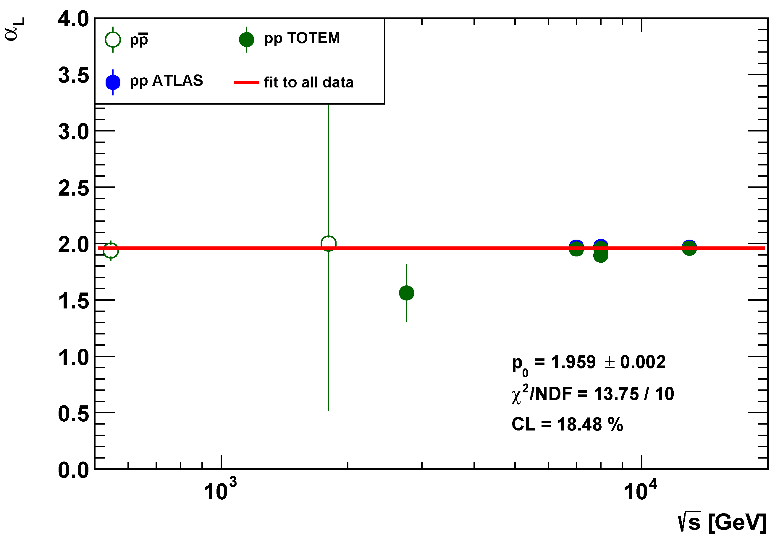
The ${\alpha }_L\left(s\right)$ parameters can be fitted with an energy-independent constant ${\alpha }_L$ value, as shown in Figure 1. This average, constant value of the ${\alpha }_L$ parameter is consistent with all the measurements, with ${\alpha }_L=1.959\pm 0.002$. Although this average value is close to the Gaussian ${\alpha }_L=2$ case, which corresponds to an exponentially shaped cone of the differential cross section of elastic scattering, its error is small, and thus, the constant value of ${\alpha }_L$ is significantly less than 2. This indicates that a strongly non-exponential SL model is consistent with all the low-$\left|t\right|$ datasets cited in Table 1.

We know that the optical point parameter is proportional to the square of the total cross section [29,54], $a\left(s\right)\sim {\sigma }_{\mathrm{tot}}^2\left(s\right)$, and the total cross section is related to the square of the size parameter [29], ${\sigma }_{\mathrm{tot}}\left(s\right)\sim R^2\left(s\right)$. This leads to the relation $a\left(s\right)\sim R^4\left(s\right)$ (see more details also in Appendix A).

The “geometric picture”, based on a series of studies [62,63,64,65,66,67], motivates the ${ln}^2(s/s_0)$ behavior of the total cross section and the $ln(s/s_0)$ behavior of the size parameter. In addition, the leading ${ln}^2(s/s_0)$ term of hadronic total cross sections was obtained from lattice QCD calculations [68,69]. In the Donnachie–Landshoff approach of hadronic cross sections [70], the energy dependence is described by a sum of powers of s, ${\sum }_i{c}_i{(s/s_0)}^{{\delta }_i}$. However, it was discussed in Refs. [71,72,73,74,75,76] that models with a ${ln}^2(s/s_0)$ asymptotic term work much better than those with $ln(s/s_0)$ or ${(s/s_0)}^{\delta }$ asymptotic terms.

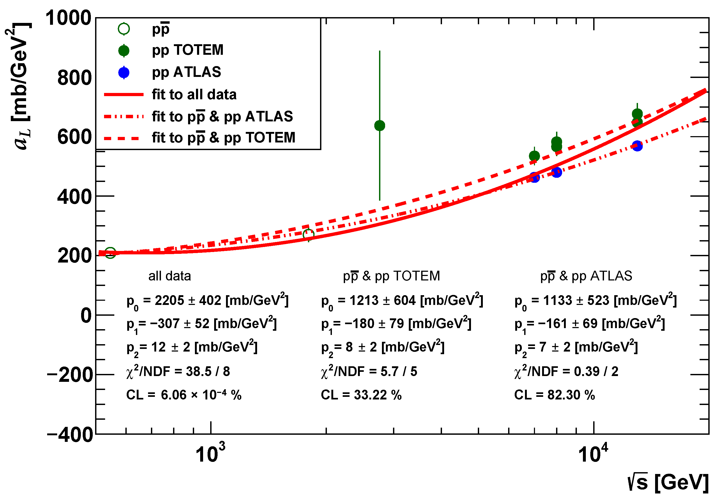
In Ref. [56], the size parameter was successfully parameterized by a ${\sum }_{i=0}^1{p}_i{ln}^i(s/s_0)$ functional form in the energy range of 546 GeV $\le \sqrt{s}\le$ 8 TeV. This would suggest a ${\sum }_{i=0}^4{p}_i{ln}^i(s/s_0)$ functional form for the energy dependence of the optical point parameter. However, in our analysis with the SL model, we find that the energy dependence of the optical point $a_L\left(s\right)$ for $p\overline{p}$ and ATLAS or for $p\overline{p}$ and TOTEM data in the energy range 0.54 TeV $\le \sqrt{s}\le 13$ TeV is compatible with a quadratically logarithmic shape,

$$a\left(s\right)=p_0+p_{1}ln\left(\frac{s}{1{\mathrm{GeV}}^2}\right)+p_2{ln}^2\left(\frac{s}{1{\mathrm{GeV}}^2}\right),$$

(21)

i.e., the corrections of the ${ln}^3(s/s_0)$ and ${ln}^4(s/s_0)$ terms are smaller than the current experimental precision. Our result for the energy dependence of the optical point $a_L\left(s\right)$ is shown in Figure 2.

For $p\overline{p}$ and ATLAS data, the values of the parameters in Equation (21) are $p_0=1213\pm 604$ mb/GeV², $p_1=-180\pm 79$ mb/GeV², and $p_2=8\pm 2$ mb/GeV², resulting in a confidence level of $33.22\%$. For $p\overline{p}$ and TOTEM data, the parameter values are $p_0=1133\pm 523$ mb/GeV², $p_1=-161\pm 69$ mb/GeV², and $p_2=7\pm 2$ mb/GeV², resulting in a confidence level of $82.30\%$. A fit by the parametrization Equation (21) that includes a parameter values for all data—$p\overline{p}$, ATLAS, and TOTEM—is statistically not acceptable since its confidence level is 6.06$\times {10}^{-4}\%$.

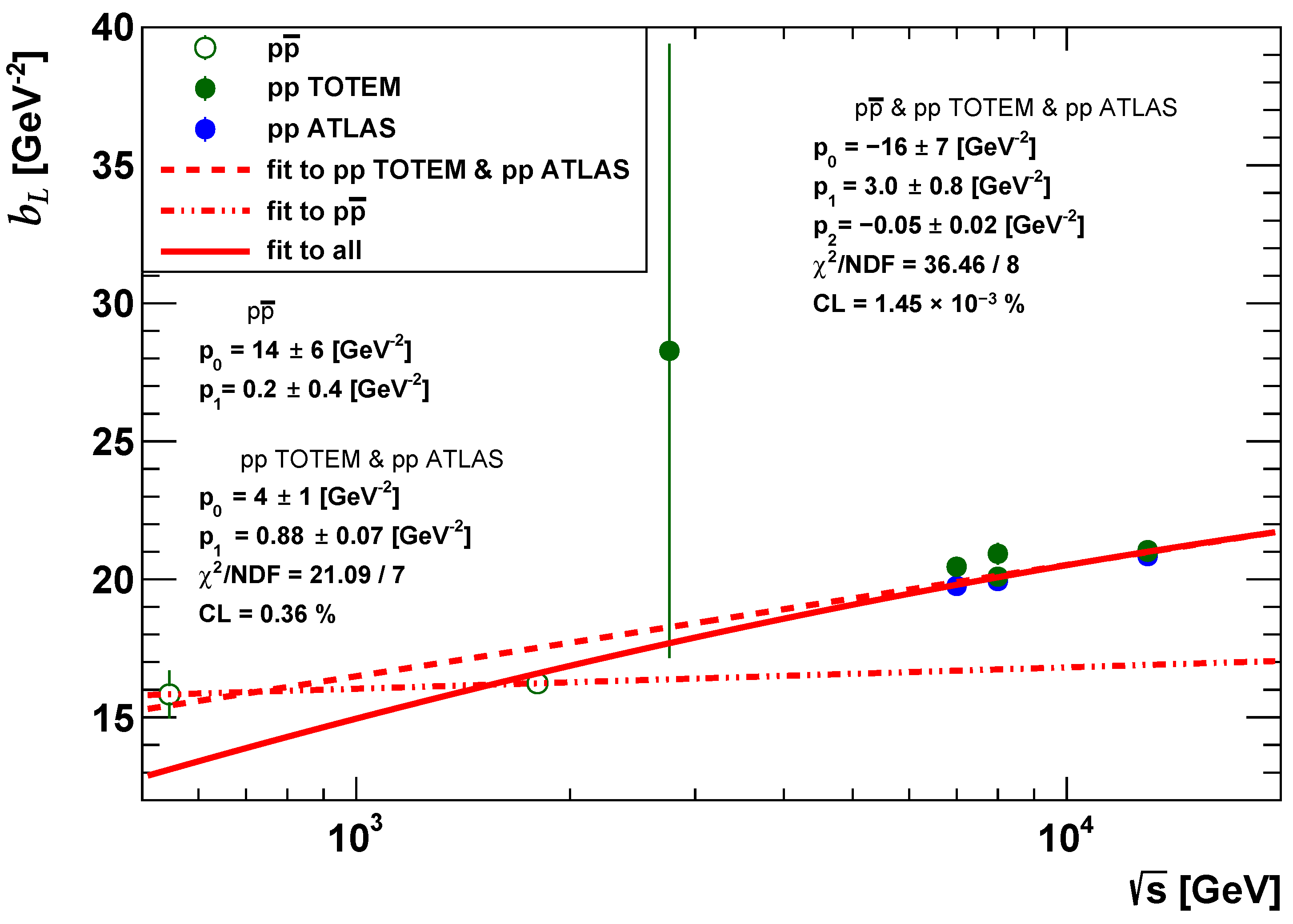
As discussed in Appendix A, the slope parameter is related to the size parameter as $b\left(s\right)=R^2\left(s\right)$. This would suggest a ${\sum }_{i=0}^2=p_i{ln}^i(s/s_0)$ functional form for the energy dependence of the optical point parameter. However, we find that for ATLAS and TOTEM $pp$ data, the energy dependence of the $b_L$ parameter is compatible with a linearly logarithmic shape,

$$b\left(s\right)=p_0+p_{1}ln\left(\frac{s}{1{\mathrm{GeV}}^2}\right),$$

(22)

with $p_0=4\pm 1$ GeV⁻² and $p_1=0.88\pm 0.07$ GeV⁻² resulting in a confidence level of $0.36\%$, as illustrated in Figure 3. This result, when taken together with the results of Figure 1 and Figure 2, suggests that ATLAS and TOTEM data in the low $-t$ region have a consistent non-exponential shape but differ in their overall normalization. A linearly logarithmic shape for the slope parameter also follows form the one-pomeron exchange Regge model [54].

The values of the $b_L$ parameter for $p\overline{p}$ data lie on the line given by Equation (22) with the parameters $p_0=14\pm 6$ GeV⁻² and $p_1=0.2\pm 0.4$ GeV⁻². These values are significantly different from the values of linearity for elastic $pp$ collisions, $p_0=4\pm 1$ GeV⁻² and $p_1=0.88\pm 0.07$ GeV⁻². The fit for the $b_L$ parameter values of all data—$p\overline{p}$, ATLAS, and TOTEM—even by the quadratic parametrization Equation (21) is statistically not acceptable, as it has too small of a confidence level of $1.45\times {10}^{-3}\%$.

5. Discussion

In this work, we fitted the low-$\left|t\right|$ elastic $pp$ and $p\overline{p}$ differential cross section in the center of mass energy range of 0.54 TeV $\le \sqrt{s}\le 13$ TeV. To do this, we used the SL model as defined by Equation (2). Another popular empirical parametrization for the low-$\left|t\right|$ non-exponential differential cross section is Equation (1). The effect of the quadratic term in the exponent of Equation (1) is reproduced in our model by an ${\alpha }_L$ parameter value less than 2.

An exponential differential cross section corresponds to a Gaussian impact parameter profile. The Gaussian distribution is the ${\alpha }_L=2$ special case of the more general Lévy $\alpha$-stable distributions. The experimentally observed non-exponential differential cross section at low-$\left|t\right|$ indicates that the impact parameter profiles, ${\tilde{\sigma }}_{in}$ and $\Gamma$, rather have Lévy $\alpha$-stable shapes at high-b, resulting in the SL model given by Equation (2). Accordingly, it may be more natural to use Equation (2) instead of Equation (1) to model the experimental data. Lévy-$\alpha$-stable-shaped source functions are extensively used in the analysis of data on heavy ion collisions, as detailed in the Introduction.

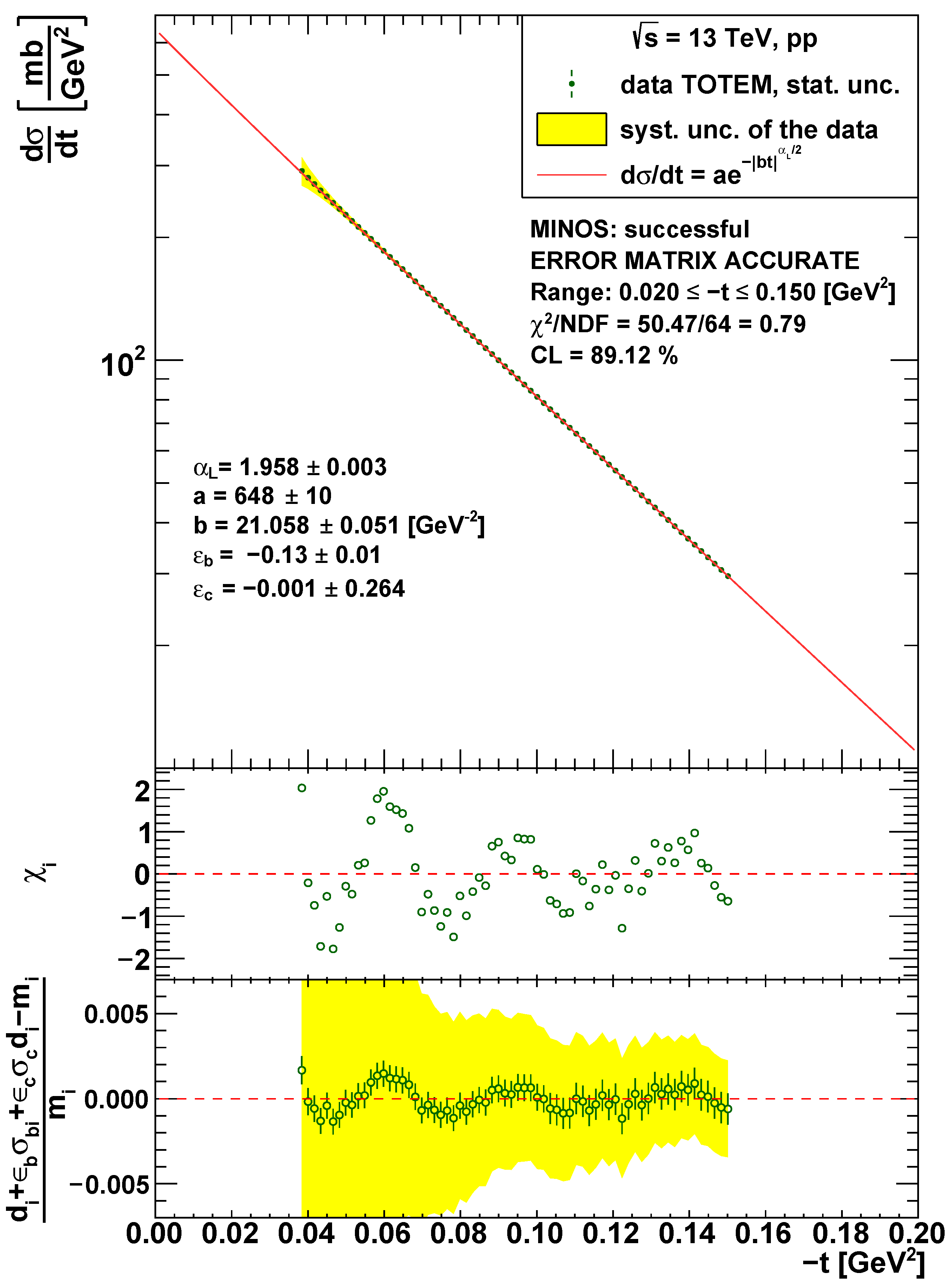
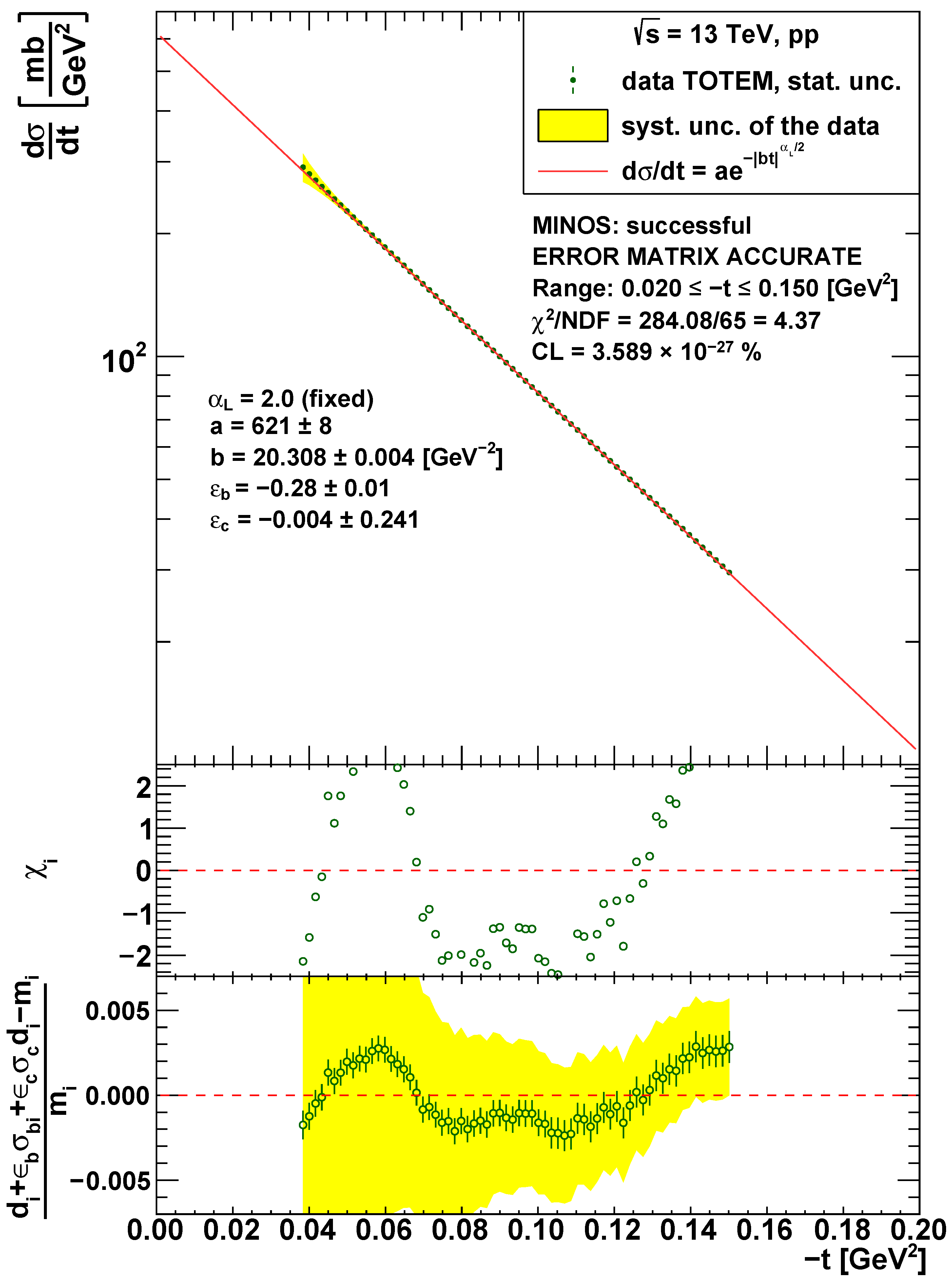
As an illustrative example, the SL model fit to the most precise TOTEM data measured at $\sqrt{s}=$ 13 TeV [10] is shown in Figure 4, and the case with ${\alpha }_L=2$ fixed is shown in Figure 5. The SL model with ${\alpha }_L=1.958\pm 0.003$ describes the 13 TeV TOTEM data with CL = 89.12%, while the ${\alpha }_L=2$ fixed case fit has a confidence level of 3.6 $\times {10}^{-27}$%. These values are not surprising if one compares the bottom panel of Figure 4 to the bottom panel of Figure 5. This result clearly shows the success of the non-exponential SL model with ${\alpha }_L<2$.

Looking at the bottom panel of Figure 4, one can observe some oscillations in the data. This oscillation is a significant effect when only the statistical errors are considered. If systematic errors are taken into account as well, this oscillation effect disappears. The SL model has a monotonically decreasing shape and describes the data with a good confidence level. This excludes the statistically significant oscillatory behavior of the data.

Let us now discuss the energy dependence of the SL model parameters. According to our analysis, surprisingly, the ${\alpha }_L$ parameter of the SL model is energy-independent, and its value is 1.959 ± 0.002, indicating a Lévy-$\alpha$-stable-shaped, power-law tail feature for impact parameter profiles ${\tilde{\sigma }}_{\mathrm{in}}$ and $\Gamma$ in the energy range 546 GeV $\le \sqrt{s}\le$ 13 TeV.

We showed in Section 4 that the energy dependence of the optical point parameter of the SL model is compatible with a quadratically logarithmic shape; however, the a parameter values determined from ATLAS and TOTEM data on $pp$ elastic scattering disagree. This discrepancy is a well-known fact, and the interpretation is that the ATLAS and TOTEM experiments use different methods to obtain the absolute normalization of the measurements [13].

We saw in Section 4 that $pp$ and $p\overline{p}$b parameter values lie in different curves. There are two alternative interpretations. The TOTEM Collaboration discussed in Ref. [77] that there is a jump in the energy dependence of the slope parameter in the energy interval of 3 GeV $\lesssim \sqrt{s}\lesssim$ 4 GeV. One of the possibilities is that the same jump is seen in our analysis as well, preventing the lower energy $p\overline{p}$ data to lie in the same curve with the higher energy LHC ATLAS and TOTEM data. The second possibility is that the difference between the $pp$ and $p\overline{p}$ slope is the effect of the odderon [78]. New $pp$ low-$\left|t\right|$ measurements at LHC at $\sqrt{s}=$ 1.8 and/or 1.96 TeV may clarify this issue.

6. Summary

We fitted the $pp$ and $p\overline{p}$ elastic differential cross section with a simple Lévy $\alpha$-stable model in the center of mass energy range of 0.54 TeV $\le \sqrt{s}\le 13$ TeV and in the four-momentum transfer range of 0.02 GeV²$\le -t\le 0.15$ GeV². We determined the energy dependence of the three parameters of the model. The Lévy index of stability, ${\alpha }_L\left(s\right)$, results are consistent with an energy-independent, constant value that is slightly but significantly smaller than 2. The energy dependence of the optical point parameter is the same for $pp$ and $p\overline{p}$ processes and has a quadratically logarithmic shape; however, because of normalization differences, TOTEM and ATLAS optical point data are inconsistent within experimental errors. Thus, they can be fitted separately from one another and, furthermore, both can be fitted together with $p\overline{p}$ data; however, the ATLAS and TOTEM optical points cannot be fitted together, neither without nor with the $p\overline{p}$ data.

In our Lévy analysis, we observe that the Lévy slope parameter $b\left(s\right)$ has different energy dependence for $pp$ and $p\overline{p}$ scattering. This may be an odderon signal [78] or the “jumping” behavior in the energy interval of 3 GeV $\lesssim \sqrt{s}\lesssim$ 4 GeV as discussed by TOTEM in Ref. [77]. New $pp$ low-$\left|t\right|$ measurements at LHC at $\sqrt{s}=$ 1.8 and/or 1.96 TeV may decide which interpretation is true. We also find that TOTEM and ATLAS slope parameter data can be fitted together with a linearly logarithmic shape, indicating that TOTEM and ATLAS data differ only in their normalization, while their shape is consistent. Similar conclusions were drawn in Ref. [79] concerning the TOTEM–ATLAS discrepancy at 13 TeV.

References

- Barbiellini, G.; Bozzo, M.; Darriulat, P.; Diambrini-Palazzi, G.; De Zorzi, G.; Fainberg, A.; Ferrero, M.I.; Holder, M.; McFarland, A.; Maderni, G.; et al. Small angle proton proton elastic scattering at very high-energies (460-GeV2 < s < 2900-GeV2). Phys. Lett. B 1972, 39, 663–667. [Google Scholar] [CrossRef]
- Nagy, E.; Orr, R.S.; Schmidt-Parzefall, W.; Winter, K.; Brandt, A.; Büsser, F.W.; Flügge, G.; Niebergall, F.; Schumacher, P.E.; Eichinger, H.; et al. Measurements of Elastic Proton Proton Scattering at Large Momentum Transfer at the CERN Intersecting Storage Rings. Nucl. Phys. B 1979, 150, 221–267. [Google Scholar] [CrossRef]
- Donnachie, A.; Landshoff, P.V. The Interest of large-t elastic scattering. Phys. Lett. B 1996, 387, 637–641. [Google Scholar] [CrossRef]
- Antchev, G. et al. [TOTEM Collaboration] Elastic differential cross-section dσ/dt at = 2.76 TeV and implications on the existence of a colourless C-odd three-gluon compound state. Eur. Phys. J. C 2020, 80, 91. [Google Scholar] [CrossRef]
- Antchev, G. et al. [TOTEM Collaboration] Measurement of proton-proton elastic scattering and total cross-section at S**(1/2) = 7-TeV. EPL Europhys. Lett. 2013, 101, 21002. [Google Scholar] [CrossRef]
- Antchev, G. et al. [TOTEM Collaboration] Evidence for non-exponential elastic proton–proton differential cross-section at low |t| and s = 8 TeV by TOTEM. Nucl. Phys. B 2015, 899, 527–546. [Google Scholar] [CrossRef]
- Antchev, G. et al. [TOTEM Collaboration] Measurement of elastic pp scattering at = 8 TeV in the Coulomb–nuclear interference region: Determination of the æ-parameter and the total cross-section. Eur. Phys. J. C 2016, 76, 661. [Google Scholar] [CrossRef]
- Antchev, G. et al. [TOTEM Collaboration] Characterisation of the dip-bump structure observed in proton–proton elastic scattering at s = 8 TeV. Eur. Phys. J. C 2022, 82, 263. [Google Scholar] [CrossRef]
- Antchev, G. et al. [TOTEM Collaboration] First determination of the ρ parameter at = 13 TeV: Probing the existence of a colourless C-odd three-gluon compound state. Eur. Phys. J. C 2019, 79, 785. [Google Scholar] [CrossRef]
- Antchev, G. et al. [TOTEM Collaboration] Elastic differential cross-section measurement at = 13 TeV by TOTEM. Eur. Phys. J. C 2019, 79, 861. [Google Scholar] [CrossRef]
- Aad, G. et al. [ATLAS Collaboration] Measurement of the total cross section from elastic scattering in pp collisions at = 7 TeV with the ATLAS detector. Nucl. Phys. B 2014, 889, 486–548. [Google Scholar] [CrossRef]
- Aaboud, M. et al. [ATLAS Collaboration] Measurement of the total cross section from elastic scattering in pp collisions at = 8 TeV with the ATLAS detector. Phys. Lett. B 2016, 761, 158–178. [Google Scholar] [CrossRef]
- Aad, G. et al. [ATLAS Collaboration] Measurement of the total cross section and ρ-parameter from elastic scattering in pp collisions at = 13 TeV with the ATLAS detector. Eur. Phys. J. C 2023, 83, 441. [Google Scholar] [CrossRef]
- Breakstone, A.; Crawley, H.B.; Dallavalle, G.M.; Doroba, K.; Drijard, D.; Fabbri, F.; Firestone, A.; Fischer, H.G.; Frehse, H.; Geist, W.; et al. A Measurement of p and pp Elastic Scattering in the Dip Region at = 53-GeV. Phys. Rev. Lett. 1985, 54, 2180. [Google Scholar] [CrossRef]
- Bozzo, M. et al. [UA4 Collaboration] Elastic Scattering at the CERN SPS Collider Up to a Four Momentum Transfer of 1.55-GeV2. Phys. Lett. B 1985, 155, 197–202. [Google Scholar] [CrossRef]
- Bernard, D. et al. [UA4 Collaboration] Large t Elastic Scattering at the CERN SPS Collider at = 630-GeV. Phys. Lett. B 1986, 171, 142–144. [Google Scholar] [CrossRef]
- Abazov, V.M. et al. [D0 Collaboration] Measurement of the differential cross section dσ/dt in elastic scattering at = 1.96 TeV. Phys. Rev. D 2012, 86, 012009. [Google Scholar] [CrossRef]
- Battiston, R. et al. [UA4 Collaboration] Proton-Anti-proton Elastic Scattering at Four Momentum Transfer Up to 0.5-GeV2 at the CERN SPS Collider. Phys. Lett. B 1983, 127, 472. [Google Scholar] [CrossRef]
- Bozzo, M. et al. [UA4 Collaboration] Measurement of the Proton-anti-Proton Total and Elastic Cross-Sections at the CERN SPS Collider. Phys. Lett. B 1984, 147, 392. [Google Scholar] [CrossRef]
- Cohen-Tannoudji, G.; Ilyin, V.V.; Jenkovszky, L.L. A model for the pomeron trajectory. Lett. Nuovo Cim. 1972, 5S2, 957–962. [Google Scholar] [CrossRef]
- Anselm, A.A.; Gribov, V.N. Zero pion mass limit in interactions at very high-energies. Phys. Lett. B 1972, 40, 487–490. [Google Scholar] [CrossRef]
- Tan, C.I.; Tow, D.M. Can Pions Be the Dominant Linkage in Multiperipheral Cluster Models? Phys. Lett. B 1975, 53, 452–456. [Google Scholar] [CrossRef]
- Khoze, V.A.; Martin, A.D.; Ryskin, M.G. Soft diffraction and the elastic slope at Tevatron and LHC energies: A MultiPomeron approach. Eur. Phys. J. C 2000, 18, 167–179. [Google Scholar] [CrossRef]
- Jenkovszky, L.; Lengyel, A. Low-|t| structures in elastic scattering at the LHC. Acta Phys. Polon. B 2015, 46, 863–878. [Google Scholar] [CrossRef]
- Fagundes, D.A.; Jenkovszky, L.; Miranda, E.Q.; Pancheri, G.; Silva, P.V.R.G. Fine structure of the diffraction cone: From ISR to the LHC. In Proceedings of the Gribov-85 Memorial Workshop on Theoretical Physics of XXI Century, Chernogolovka, Russia, 17–20 June 2015. [Google Scholar] [CrossRef]
- Jenkovszky, L.; Szanyi, I.; Tan, C.I. Shape of Proton and the Pion Cloud. Eur. Phys. J. A 2018, 54, 116. [Google Scholar] [CrossRef]
- Kohara, A.K. Forward scattering amplitudes of pp and with crossing symmetry and scaling properties. J. Phys. G 2019, 46, 125001. [Google Scholar] [CrossRef]
- Kohara, A.K.; Ferreira, E.; Rangel, M. The interplay of hadronic amplitudes and Coulomb phase in LHC measurements at 13 TeV. Phys. Lett. B 2019, 789, 1–6. [Google Scholar] [CrossRef]
- Csörgő, T.; Hegyi, S.; Szanyi, I. Lévy α-Stable Model for the Non-Exponential Low-|t| Proton–Proton Differential Cross-Section. Universe 2023, 9, 361. [Google Scholar] [CrossRef]
- Uchaikin, V.V.; Zolotarev, V.M. Chance and Stability: Stable Distributions and Their Applications; Walter de Gruyter: Berlin, Germany, 2011. [Google Scholar]
- Tsallis, C.; Levy, S.V.F.; Souza, A.M.C.; Maynard, R. Statistical-Mechanical Foundation of the Ubiquity of Levy Distributions in Nature. Phys. Rev. Lett. 1995, 75, 3589–3593. [Google Scholar] [CrossRef]
- Prato, D.; Tsallis, C. Nonextensive foundation of Levy distributions. Phys. Rev. E 1999, 60, 2398. [Google Scholar] [CrossRef]
- Nolan, J.P. Univariate Stable Distributions; Springer: Berlin/Heidelberg, Germany, 2020. [Google Scholar]
- Wilk, G.; Wlodarczyk, Z. On the interpretation of nonextensive parameter q in Tsallis statistics and Levy distributions. Phys. Rev. Lett. 2000, 84, 2770. [Google Scholar] [CrossRef]
- Brax, P.; Peschanski, R.B. Levy stable law description of intermittent behavior and quark-gluon plasma phase transitions. Phys. Lett. B 1991, 253, 225–230. [Google Scholar] [CrossRef]
- Zhang, Y.; Liu, L.S.; Wu, Y.F. Levy stability for anisotropic dynamical fluctuation in high-energy multiparticle production. Z. Phys. C 1996, 71, 499–502. [Google Scholar] [CrossRef]
- Csörgő, T.; Hegyi, S.; Zajc, W.A. Bose-Einstein correlations for Levy stable source distributions. Eur. Phys. J. C 2004, 36, 67–78. [Google Scholar] [CrossRef]
- Csörgő, T.; Kittel, W.; Metzger, W.J.; Novák, T. Parametrization of Bose-Einstein Correlations and Reconstruction of the Space-Time Evolution of Pion Production in e+e− Annihilation. Phys. Lett. B 2008, 663, 214–216. [Google Scholar] [CrossRef]
- Achard, P. et al. [The L3 Collaboration] Test of the τ-Model of Bose-Einstein Correlations and Reconstruction of the Source Function in Hadronic Z-boson Decay at LEP. Eur. Phys. J. C 2011, 71, 1648. [Google Scholar] [CrossRef]
- Kurgyis, B.; Kincses, D.; Nagy, M.; Csanád, M. Coulomb Corrections for Bose–Einstein Correlations from One- and Three-Dimensional Lévy-Type Source Functions. Universe 2023, 9, 328. [Google Scholar] [CrossRef]
- Adare, A. et al. [PHENIX Collaboration] Lévy-stable two-pion Bose-Einstein correlations in = 200 GeV Au+Au collisions. Phys. Rev. C 2018, 97, 064911, Erratum in Phys. Rev. C 2023, 108, 049905. [Google Scholar] [CrossRef]
- Schegelsky, V.A. Levy Analysis of Bose–Einstein Correlation in pp Collisions at s = 7 TeV Measured with the ATLAS. Phys. Part. Nucl. Lett. 2019, 16, 503–507. [Google Scholar] [CrossRef]
- Tumasyan, A. et al. [CMS Collaboration] Two-particle Bose-Einstein correlations and their Lévy parameters in PbPb collisions at = 5.02 TeV. arXiv 2023, arXiv:2306.11574. [Google Scholar] [CrossRef]
- Lökös, S. Centrality dependent Lévy-stable two-pion Bose-Einstein correlations in = 200 GeV Au+Au collisions at the PHENIX experiment. Universe 2018, 4, 31. [Google Scholar] [CrossRef]
- Kincses, D. Pion interferometry with Lévy-stable sources in = 200 GeV Au+Au collisions at STAR. arXiv 2024, arXiv:2401.11169. [Google Scholar] [CrossRef]
- Pórfy, B. Lévy HBT Results at NA61/SHINE. Universe 2019, 5, 154. [Google Scholar] [CrossRef]
- Porfy, B. Femtoscopic Correlation Measurement with Symmetric Lévy-Type Source at NA61/SHINE. Universe 2023, 9, 298. [Google Scholar] [CrossRef]
- Csanád, M.; Kincses, D. Femtoscopy with Lévy sources from SPS through RHIC to LHC. Universe 2024, 10, 54. [Google Scholar] [CrossRef]
- Novák, T.; Csörgő, T.; Eggers, H.C.; de Kock, M. Model independent analysis of nearly Lévy correlations. Acta Phys. Polon. Supp. 2016, 9, 289. [Google Scholar] [CrossRef]
- Csörgő, T.; Pasechnik, R.; Ster, A. Proton structure and hollowness from Lévy imaging of pp elastic scattering. Eur. Phys. J. C 2020, 80, 126. [Google Scholar] [CrossRef]
- Csörgő, T.; Pasechnik, R.; Ster, A. Odderon and proton substructure from a model-independent Lévy imaging of elastic pp and collisions. Eur. Phys. J. C 2019, 79, 62. [Google Scholar] [CrossRef] [PubMed]
- Glauber, R. Lectures in theoretical physics, ed. WE Brittin and LG Dunham. Interscience 1959, 1, 315. [Google Scholar]
- Glauber, R. Theory of high energy hadron-nucleus collisions. In Proceedings of the High-Energy Physics and Nuclear Structure: Proceedings of the Third International Conference on High Energy Physics and Nuclear Structure sponsored by the International Union of Pure and Applied Physics, held at Columbia University, New York, NY, USA, 8–12 September 1969; Springer: Berlin/Heidelberg, Germany; pp. 207–264.
- Barone, V.; Predazzi, E. High-Energy Particle Diffraction; Springer: Berlin, Germany, 2002. [Google Scholar]
- Glauber, R.J.; Velasco, J. Multiple Diffraction Theory of Scattering at 546-GeV. Phys. Lett. B 1984, 147, 380–384. [Google Scholar] [CrossRef]
- Csörgő, T.; Szanyi, I. Observation of Odderon effects at LHC energies: A real extended Bialas–Bzdak model study. Eur. Phys. J. C 2021, 81, 611. [Google Scholar] [CrossRef]
- Bialas, A.; Bzdak, A. Constituent quark and diquark properties from small angle proton-proton elastic scattering at high energies. Acta Phys. Polon. B 2007, 38, 159–168. [Google Scholar]
- Nemes, F.; Csörgő, T.; Csanád, M. Excitation function of elastic pp scattering from a unitarily extended Bialas–Bzdak model. Int. J. Mod. Phys. A 2015, 30, 1550076. [Google Scholar] [CrossRef]
- Szanyi, I.; Csörgő, T. The ReBB model and its H(x) scaling version at 8 TeV: Odderon exchange is a certainty. Eur. Phys. J. C 2022, 82, 827. [Google Scholar] [CrossRef]
- Adare, A. et al. [PHENIX Collaboration] Quantitative Constraints on the Opacity of Hot Partonic Matter from Semi-Inclusive Single High Transverse Momentum Pion Suppression in Au+Au collisions at = 200-GeV. Phys. Rev. C 2008, 77, 064907. [Google Scholar] [CrossRef]
- Amos, N.A. et al. [E-710 Collaboration] p Elastic Scattering at s = 1.8-TeV from |t| = 0.034-GeV/c2 to 0.65-GeV/c2. Phys. Lett. B 1990, 247, 127–130. [Google Scholar] [CrossRef]
- Cheng, H.; Wu, T.T. High-energy elastic scattering in quantum electrodynamics. Phys. Rev. Lett. 1969, 22, 666. [Google Scholar] [CrossRef]
- Cheng, H.; Wu, T.T. High-energy collision processes in quantum electrodynamics. i. Phys. Rev. 1969, 182, 1852–1867. [Google Scholar] [CrossRef]
- Cheng, H.; Wu, T.T. High-energy collision processes in quantum electrodynamics. ii. Phys. Rev. 1969, 182, 1868–1872. [Google Scholar] [CrossRef]
- Cheng, H.; Wu, T.T. Expanding Protons: Scattering at High-Energies; Mit Pr: Cambridge, MA, USA, 1987. [Google Scholar]
- Bourrely, C.; Soffer, J.; Wu, T.T. A New Impact Picture for Low and High-Energy Proton Proton Elastic Scattering. Phys. Rev. D 1979, 19, 3249. [Google Scholar] [CrossRef]
- Bourrely, C.; Soffer, J.; Wu, T.T. Do we understand near-forward elastic scattering up to TeV energies? Int. J. Mod. Phys. A 2015, 30, 1542006. [Google Scholar] [CrossRef]
- Giordano, M.; Meggiolaro, E.; Moretti, N. Asymptotic Energy Dependence of Hadronic Total Cross Sections from Lattice QCD. J. High Energy Phys. 2012, 2012, 31. [Google Scholar] [CrossRef]
- Giordano, M.; Meggiolaro, E. Hadronic total cross sections at high energy and the QCD spectrum. J. High Energy Phys. 2014, 2014, 2. [Google Scholar] [CrossRef]
- Donnachie, S.; Dosch, G.; Landshoff, P.; Nachtmann, O. Pomeron Physics and QCD; Cambridge University Press: Cambridge, UK, 2002. [Google Scholar]
- Patrignani, C. Review of Particle Physics. Chin. Phys. C 2016, 40, 100001. [Google Scholar] [CrossRef]
- Martynov, E. Elastic pp and anti-pp scattering in the models of unitarized pomeron. Phys. Rev. D 2007, 76, 074030. [Google Scholar] [CrossRef]
- Martynov, E.; Nicolescu, B. Unified model for small-t and high-t scattering at high energies: Predictions at RHIC and LHC. Eur. Phys. J. C 2008, 56, 57–62. [Google Scholar] [CrossRef]
- Cudell, J.R.; Lengyel, A.; Martynov, E. The Soft and the hard pomerons in hadron elastic scattering at small t. Phys. Rev. D 2006, 73, 034008. [Google Scholar] [CrossRef]
- Cahn, R. Coulombic-Hadronic Interference in an Eikonal Model. Z. Phys. C 1982, 15, 253. [Google Scholar] [CrossRef]
- Martynov, E. Proton (antiproton) elastic scattering at energies from FNAL to the LHC in the tripole Pomeron-Odderon model. Phys. Rev. D 2013, 87, 114018. [Google Scholar] [CrossRef]
- Antchev, G. et al. [TOTEM Collaboration] First measurement of elastic, inelastic and total cross-section at = 13 TeV by TOTEM and overview of cross-section data at LHC energies. Eur. Phys. J. C 2019, 79, 103. [Google Scholar] [CrossRef]
- Csörgő, T.; Szanyi, I. Cross-Checking Odderon Signals at Small Values of Four-Momentum Transfer. Presentation at ISMD 2023, Gyöngyös, Hungary. Available online: https://indico.cern.ch/event/1258038/contributions/5537131/attachments/2702376/4690629/2023-08-24-Csorgo-ISMD-final.pdf (accessed on 5 March 2024).
- Petrov, V.A.; Tkachenko, N.P. ATLAS vs TOTEM: Disturbing Divergence. arXiv 2023, arXiv:2303.01058. [Google Scholar] [CrossRef]
- Block, M.M. Hadronic forward scattering: Predictions for the Large Hadron Collider and cosmic rays. Phys. Rept. 2006, 436, 71–215. [Google Scholar] [CrossRef]
- Broniowski, W.; Jenkovszky, L.; Ruiz Arriola, E.; Szanyi, I. Hollowness in pp and scattering in a Regge model. Phys. Rev. D 2018, 98, 074012. [Google Scholar] [CrossRef]
Figure 1.
The values of the parameter of the SL model at different energies from half TeV up to 13 TeV. The parameter of the model is energy-independent: its values at different energies can be fitted with a constant, 1.959 ± 0.002.
Figure 2.
The values of the optical point parameter of the SL model at different energies from half TeV up to 13 TeV.
Figure 3.
The values of the slope parameter of the SL model at different energies from half TeV up to 13 TeV.
Figure 4.
Fit to the low- differential cross section data measured by TOTEM at 13 TeV [10], with the SL model defined by Equation (2). The differential cross section data with the fitted model curve as well as the values of the fit parameters and the fit statistics are shown in the top panel. The middle panel shows the values corresponding to the data points . The bottom panel shows the relative deviation between , the data points shifted within errors by the correlation parameters of the definition Equation (18), and , the values calculated from the model.
Figure 5.
Same as Figure 1 but with fixed.