
A Simple Direct Empirical Observation of Systematic Bias of the Redshift as a Distance Indicator


Department of Computer Science, Kansas State University, Manhattan, KS 66506, USA
Universe 2024, 10(3), 129; https://doi.org/10.3390/universe10030129
Submission received: 12 February 2024
/
Revised: 1 March 2024
/
Accepted: 4 March 2024
/
Published: 6 March 2024
Abstract
:Recent puzzling observations, such as the tension, large-scale anisotropies, and massive disk galaxies at high redshifts, have been challenging the standard cosmological model. While one possible explanation is that the standard model is incomplete, other theories are based on the contention that the redshift model as a distance indicator might be biased. These theories can explain the recent observations, but they are challenged by the absence of a direct empirical reproducible observation that the redshift model can indeed be inconsistent. Here, I describe a simple experiment that shows that the spectra of galaxies depend on their rotational velocity relative to the rotational velocity of the Milky Way. Moreover, it shows that the redshift of galaxies that rotate in the opposite direction relative to the Milky Way is significantly smaller compared with the redshift of galaxies that rotate in the same direction relative to the Milky Way (p < 0.006). Three different datasets were used independently, each one was prepared in a different manner, and all of them showed similar redshift bias. A fourth dataset of galaxies from the Southern Galactic pole was also analyzed and shows similar results. All four datasets are publicly available. While a maximum average z difference of ∼0.012 observed with galaxies of relatively low redshift (z < 0.25) is not extreme, the bias is consistent and canpotentially lead to explanations to puzzling observations such as the tension.
1. Introduction
Recent observations have shown unexplained tensions and anomalies at cosmological scales. For instance, the determined by the cosmic microwave background (CMB) radiation is different from the determined by using Ia supernovae and the redshift of their host galaxies [1,2,3,4,5,6,7,8]. The relatively new JWST provides unprecedented imaging power, showing massive disk galaxies with mature stellar populations at unexpectedly high redshifts that can be as high as 15 [9]. In fact, the presence of large disk galaxies at unexpectedly high redshifts was also reported before JWST saw its first light [10]. The existence of these galaxies is unexpected, as pre-JWST analyses predicted that such galaxies do not exist according to CDM cosmology [11] and therefore were not expected to be observed.
These unexpected observations challenge our understanding of the Universe. If the common distance indicators are complete and fully accurate, the standard cosmological theories are incomplete. Similarly, if the standard cosmological model is complete, it is not possible that the distance indicators currently used are fully accurate. Therefore, assuming that all distance indicators are reliable and consistent, explaining these observations might reinforce certain modifications of some of the foundations of cosmology. But in addition to theories that shift from the standard cosmological model, other theories are based on the contention that the redshift as a distance indicator at cosmological scales might be biased [12,13,14,15,16,17,18]. While the assumption that the redshift might be biased or inconsistent can explain these observations without modifying the standard model, there is currently no clear reproducible empirical evidence that the redshift might indeed be biased.
The redshift of a luminous moving object is determined by the linear component of the Doppler shift effect. But because galaxies have rotational velocity in addition to their linear velocity, their redshift can also be affected by the rotational velocity, as the rotational velocity of a luminous object also leads to a Doppler shift effect [19,20,21].
Since the rotational velocity of a galaxy is far smaller than its linear velocity relative to Earth, the rotational velocity component of the Doppler shift is often ignored when determining the distance of a galaxy. But while the Doppler shift effect driven by the rotational velocity of the galaxy is expected to be subtle, that has not yet been tested. It should also be mentioned that the physics of galaxy rotation is one of the most mysterious observations, and its nature cannot be explained unless making assumptions such as dark matter [22,23,24,25], modified Newtonian dynamics (MOND) [26,27,28,29,30,31,32,33,34,35], or other theories [36,37,38,39,40,41,42,43,44,45]. But despite over a century of research, there is still no single clear proven explanation for the physics of galaxy rotation [36,46,47,48,49,50,51,52,53,54,55,56,57,58,59], and that phenomenon is still not fully understood.
The purpose of the simple experiment described in this paper is to test the impact of the rotational velocity component of galaxies on the Doppler shift effect, and consequently, on the redshift as a distance indicator. Section 2 describes the data used in the experiment, Section 3 provides the results of the analysis, Section 4 compares the results shown in Section 3 with several other datasets collected by different methods and different telescope systems, and Section 5 discusses possible explanations in light of recently observed anisotropies and current cosmological theories.
2. Data
The experiment is based on one primary dataset and two additional independent datasets of galaxies from the Northern Galactic pole with which the results are compared. Each of these datasets was prepared in a different manner. A fourth dataset of galaxies from the Southern Galactic pole is also used for comparison, as discussed in Section 4.3.
The primary dataset contains SDSS DR8 galaxies with spectra sorted by their direction of rotation, as explained and used in [60]. Instead of using galaxies in the entire SDSS footprint, this experiment is focused on galaxies that rotate in the same direction relative to the Milky Way and galaxies that rotate in the opposite direction relative to the Milky Way. Therefore, only galaxies that are close to the Galactic pole are used, and the field is limited to degrees, centered at the Northern Galactic pole. Obviously, because the Milky Way rotates around its own pole, galaxies that are close to the galactic pole rotate either in the same direction relative to the galactic pole or in the opposite direction relative to the galactic pole. The analysis included objects with spectra in SDSS DR8 that have an r magnitude of less than 19 and a Petrosian radius of at least 5.5″. The redshift of the galaxies in that initial set was limited to z < 0.3 and the redshift error to smaller than . That selection eliminated the possible effect of bad redshift values, which in some cases can be very high and skew the dataset. The initial set of galaxies that meet these criteria in that field contained 52,328.
The process by which the galaxies were sorted by their direction of rotation is explained in detail in [60] and is similar to the process of annotating galaxies imaged by other telescopes [61,62,63,64,65,66,67]. In summary, the annotation is conducted using the Ganalyzer algorithm [68], where each galaxy image is transformed into its radial intensity plot such that the value of the pixel at Cartesian coordinates in the radial intensity plot is the median value of the 5 × 5 pixels at coordinates in the original galaxy image, where r is the radial distance measured in percentage of the galaxy radius, is the polar angle in degrees relative to the galaxy center, and is the coordinates of the galaxy center. A peak detection algorithm is then applied to the rows in the radial intensity plot, and the direction of the peaks determines the direction of the curves of the galaxy arms.
Figure 1 displays examples of the original galaxy images, their radial intensity plots, and the detected peaks. The direction of the curves of the arms is determined by the sign of the slope. Based on previous experiments [60,62,63,64,65,66,67], to avoid incorrect annotations, a direction was determined only for galaxies that had at least 30 peaks and are identified in the radial intensity plot. If fewer than 30 peaks were identified, the galaxy was not used, as its direction of rotation cannot be identified. The algorithm is described with experimental results in [68], as well as [62,63,64,65,66].
The primary advantage of the algorithm is that its simple “mechanical” nature makes it fully symmetric. Experiments of mirroring the galaxy images lead to identical inverse results compared with when using the original images [61,62,63,64,65,66].
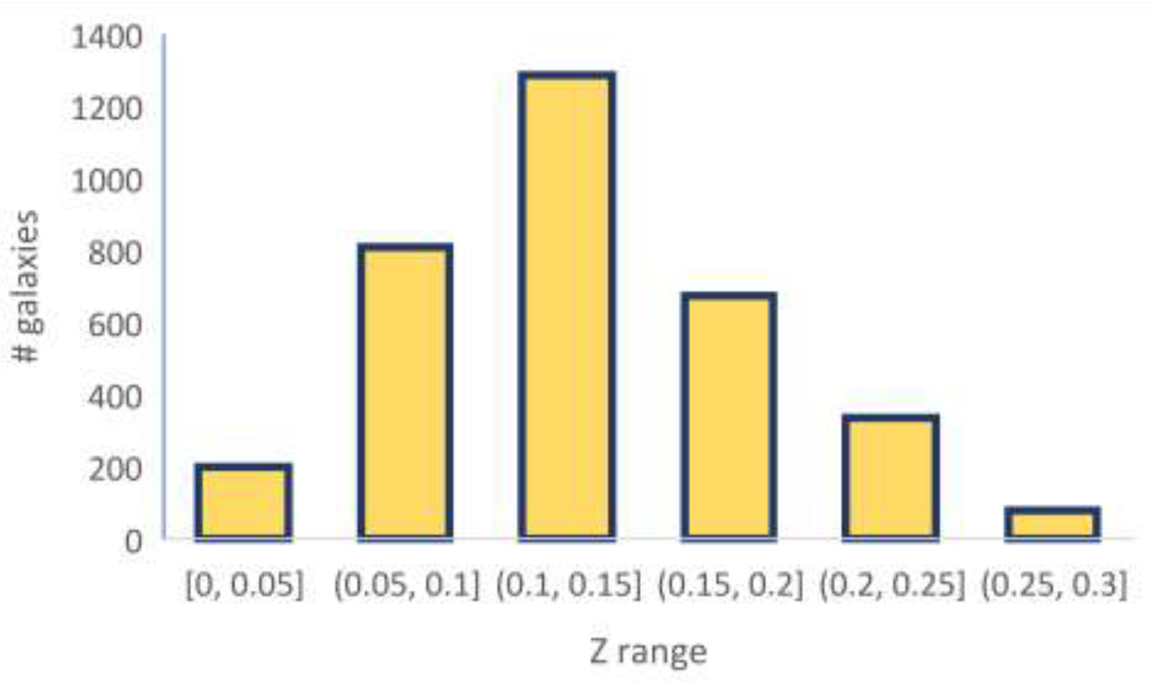
After applying the algorithm to the galaxy images, the final dataset included 1642 galaxies with identifiable directions of rotation, such that 817 galaxies rotate clockwise, and 825 galaxies rotate counterclockwise. Applying the algorithm to the mirrored images led to an identical inverse dataset. Testing a random subset of 200 galaxies showed that all galaxies were annotated correctly. Figure 2 shows the redshift distribution of the galaxies. The dataset is available at https://people.cs.ksu.edu/~lshamir/data/zdifference/ (accessed on 1 March 2024). In addition to this dataset, two other previous public datasets were used, as described in Section 4.
3. Results
Table 1 shows the redshift differences in the 20 × 20-degree field centered at the Northern Galactic pole, as well as the smaller 10 × 10-degree field. The errors are the standard error of the mean, computed by , where N is the number of galaxies. The mean redshift of the galaxies in the dataset described in Section 2 that rotate in the same direction relative to the Milky Way (MW) is 0.09545 ± 0.0017, while the mean redshift of the galaxies in the same field that rotate in the opposite direction relative to the Milky Way (OMW) is 0.08895 ± 0.0016. This shows a of ∼0.0065 ± 0.0023 between galaxies that rotate in the same direction relative to the Milky Way and galaxies that rotate in the opposite direction relative to the Milky Way.
By applying a simple Student t-test, the two-tailed probability that the two means are different by mere chance is ( 0.0058). To verify the statistical significance, a simulation test was also performed. The simulation randomly selected a set of 817 galaxies and another set of 825 galaxies regardless of their spin direction. That was repeated 100,000 times, and in each run, the mean redshift of the galaxies in the first set was compared with the mean redshift of the galaxies in the second set. In 614 of the runs, the difference between the mean redshifts of the two sets was greater than 0.0016. This provides a probability of 0.0061, which is similar to the two-tailed t-test probability. The similarity between the probability of the t-test and the probability of the simulation is not surprising but provides consistency and ensures that the t-test P-values are not driven by a certain unusual distribution of the redshift values.
If the observed difference in redshift is driven by the rotational velocity of the observed galaxy relative to the rotational velocity of the Milky Way, the difference should increase when the observed galaxies are closer to the Galactic pole. As Table 1 shows, indeed increases in the 10×10 field. Despite the lower number of galaxies, the difference is still statistically significant.
If the redshift difference peaks at the Northern Galactic pole, it is expected that galaxies that are on or close to the galactic pole would show higher redshift difference, while when using galaxies that are more distant from the Galactic pole the redshift difference would decrease. Figure 3 shows the change in when the size of the field centered at the Galactic pole changes.
As the figure shows, the decreases as the field gets larger. That can be explained by the fact that when the field gets larger, it includes more galaxies that are more distant from the Galactic pole. While it does not fully prove a link to the rotational velocity of these galaxies relative to the Milky Way, that observation is in agreement with the contention that the redshift difference is linked to the rotational velocity of the galaxies relative to the rotational velocity of the Milky Way. The figure includes two graphs. The first shows all galaxies inside the field. For instance, when the field size is 20 × 20 degrees, it also includes the galaxies inside the 10 × 10-degree field centered at the Galactic pole. The other analysis excludes overlapping galaxies so that a galaxy can only be used in one field. That is, the galaxies in the 20 × 20-degree field centered at the Galactic pole exclude the galaxies in the 10 × 10-degree field. That provides analysis with independent sets of galaxies that do not overlap. The analysis also shows a small of ∼0.002 when the dataset includes galaxies that are more distant from the Galactic pole, but it is smaller compared with the observed when the set of galaxies is limited to galaxies closer to the Galactic pole.
To test a possible change in different redshift ranges, the galaxies in the 20 × 20 field centered at the Galactic pole were separated into galaxies with a redshift lower than 0.1 and a redshift greater than 0.1. Using 0.1 for separating the dataset into lower redshift and higher redshift galaxies provided two sets, one with 1012 galaxies with z < 0.1 and another dataset of 630 galaxies with z > 0.1. Table 2 shows the differences in redshift when the galaxies are separated into the two different redshift ranges. The of the galaxies where is 0.0028 ± 0.0013, while when , the is 0.0053 ± 0.0028. The t-test probability that the difference occurs by chance is P ≃ 0.51 and therefore not statistically significant. While not statistically significant, the dataset used here might not be sufficiently large to provide statistically significant conclusions regarding the in the different redshift ranges, if such indeed exist.
Table 3 shows the differences between the flux on the different filters, taken from the specObjAll table in SDSS DR8. The spectrum flux difference shows a consistent difference of ∼10% across the different filters. Unlike the redshift, the differences in the flux of the specific filters are not statistically significant, and therefore, a definite conclusion about the flux differences cannot be made.
4. Comparison with Other Datasets
The annotation algorithm used to sort the galaxies by their direction of rotation as discussed in Section 2 is simple and symmetric, and there is no known bias that can prefer the redshift of a certain set of galaxies as annotated by the algorithm. Also, experimenting with the same images when the images were mirrored leads to inverse results, as also shown in detail in [61,62,63,64,65,66,69]. To further test for a possible impact of unknown or unexpected biases in the annotation process, two additional annotation methods were used to test whether these algorithms provide different results.
4.1. Comparison with Annotations by Galaxy Zoo
The first annotation method that was used is the crowdsourcing-based Galaxy Zoo 1 [70]. In Galaxy Zoo, anonymous volunteers used a web-based interface to sort galaxy images by their direction of rotation. After several years of work by over 100,000 volunteers, a relatively large set of over galaxies were annotated. One of the downsides of Galaxy Zoo was that in the vast majority of the cases, the volunteers who annotated the galaxies made conflicting annotations, and the disagreement between the annotators made it difficult to use the majority of the galaxies. Another substantial downside is that the annotations were subjected to the bias of human perception, which is very difficult to model and fully understand, challenging the reliability of the annotations as a tool for primary science. Despite these known weaknesses, there is no known human perceptual bias that would associate galaxies with lower redshift to a certain direction of rotation. Therefore, although Galaxy Zoo might not necessarily be considered a complete tool when used as the sole dataset, comparing it with Galaxy Zoo can provide an indication of whether a different annotation method leads to the different results shown in Section 3.
Because the annotations of the volunteers often disagree with each other, Galaxy Zoo defined the “superclean” criterion as galaxies that 95% of the human annotators agree on the annotation. That is, if 95% of the annotations or more are for a galaxy that rotates clockwise, the annotation is considered “superclean”. While these annotations are normally correct, only 1.7% of the galaxies annotated by Galaxy Zoo 1 meet that criterion. Out of the 667,944 galaxies in the specZoo table in SDSS DR8, just 324 galaxies meet that criterion and are also inside the 20 × 20-degree field centered at the Northern Galactic pole.
The mean z of the Galaxy Zoo 1 galaxies that rotate in the same direction relative to the Milky Way in that field is 0.073834 ± 0.0041. The mean z of the galaxies that rotate in the opposite direction relative to the Milky Way is 0.068292 ± 0.00348. That shows a of 0.00554, which is similar in both direction and magnitude to the of 0.0065 observed with the dataset described in Section 2. The one-tailed p-value of that difference to occur by mere chance is 0.15. This is not statistically significant, and it can be attributed to the small size of the dataset, but the similar in both direction and magnitude shows consistency between the annotation methods. From the 324 galaxies annotated by Galaxy Zoo, 263 were also included in the dataset described in Section 2. The value of the comparison is therefore not from analyzing a new dataset but from using a different annotation method that is independent of the method used in Section 2 and therefore not subjected to the same possible unknown or unexpected biases in that method if such exist. An analysis of a completely different dataset acquired by a different telescope system that does not have any overlap with the SDSS dataset is described in Section 4.3.
4.2. Comparison with Annotations by SpArcFiRe
Another dataset that is used is the dataset of SDSS galaxies annotated by the SpArcFiRe (Scalable Automated Detection of Spiral Galaxy Arm) algorithm [71,72]. SpArcFiRe is implemented by an open-source software (https://github.com/waynebhayes/SpArcFiRe (accessed on 1 March 2024)), and the method is described in detail in [71]. In summary, the algorithm first identifies arm segments in the galaxy image and then fits these segments to logarithmic spiral arcs to determine the direction of rotation based on the curves of the arms. One of the advantages of SpArcFiRe is that it is not based on data-driven machine learning or deep learning approaches that are difficult to analyze, and it is therefore not subjected to the complex biases that are often very difficult to notice [73]. The downside of SpArcFiRe is that it has an annotation error of about 15% [66]. More importantly, since SpArcFiRe is a relatively sophisticated algorithm, it is more difficult to ensure that it is completely symmetric, and in some seldom cases, a mirrored galaxy image is not annotated as rotating in the opposite direction compared with the original image. That characteristic of the algorithm is discussed in the appendix of [72]. This weakness of the algorithm can be addressed by repeating the analysis twice, such that in the first experiment the original images are used, and in the second experiment, the mirrored images are used. Then, the results of the two experiments can be compared. While that practice might not be ideal, it can be used to compare the results with the results shown in Section 3.
The dataset used here is the dataset of spiral galaxies annotated in SpArcFiRe used in [66], which is a reproduction of the experiment described in [72]. As explained in [72], the set of galaxies is the same set of galaxies selected for annotation in [70], although the manual annotations are not used in any form in the analysis. The dataset is available at https://people.cs.ksu.edu/~lshamir/data/sparcfire (accessed on 1 March 2024). More details about the dataset are available in [66].
The dataset was prepared with the original images, and then again with the mirrored galaxy images. The dataset prepared with the original images contains 138,940 galaxies, and the dataset prepared with the mirrored images contains 139,852 galaxies. That difference is expected due to the fact that the SpArcFiRe method is not fully symmetric, as explained in the appendix of [72]. All of the galaxies used in the experiment have spectra and therefore can be used to compare the redshift. As before, galaxies with a redshift greater than 0.3 or a redshift error greater than were ignored. Table 4 shows the mean redshift in the 10 × 10 field centered at the Northern Galactic pole and in the 20 × 20 field, for both the original images and the mirrored images.
As the table shows, both the original images and the mirrored images show consistent results. These results are also consistent with the results shown in Section 3. The is lower than the observed with the dataset used in Section 3, and that could be due to the certain error rate of the annotations made by the SpArcFiRe algorithm, which is expected to weaken the signal as also shown quantitatively in Section 7.1 in [74]. To test for the effect of the annotation error, the dataset described in Section 2 was used such that 15% of the galaxies were assigned intentionally with the wrong spin direction. That reduced the from 0.0065, as shown in Section 3 to 0.0032 ± 0.0023, which is closer to the value shown in Table 4, and within 1 statistical fluctuation from it. This also shows that the magnitude of the depends on the accuracy of the annotation, which is another indication of the link between the spin direction of the galaxies and the .
4.3. Comparison with Galaxies from the Southern Galactic Pole
The data used in the experiments described above were all taken from the Northern Hemisphere, and the galaxies it contains are around the Northern Galactic pole. To verify the observed redshift difference, it is also required to test if it exists in the Southern Galactic pole as well. If the observed difference in redshift is also observed in the Southern Galactic pole, it can provide an indication that it indeed could be related to the Galactic pole. Since the three experiments above all used data collected by SDSS, using a different telescope can show that the difference is not driven by some unknown or unexpected anomaly in a specific telescope system. Also, a dataset of galaxies from the Southern Galactic pole will have no overlap with the three datasets of SDSS galaxies used above.
The set of galaxies used for the analysis are galaxies imaged by DECam used in [69] that had spectroscopic redshift through the Set of Identifications Measurements and Bibliography for Astronomical Data (SIMBAD) database [75]. As explained in [69], DECam galaxy images were acquired through the API of the DESI Legacy Survey server. The initial set of galaxies contained all objects in the South bricks of DESI Legacy Survey Data Release 8 that had a g magnitude of less than 19.5 and identified as de Vaucouleurs profiles (“DEV”), exponential disks (“EXP”), or round exponential galaxies (‘’REX”).
The galaxy images were then annotated by the Ganalyzer algorithm, as described in Section 2, and also in [69]. Unlike the other methods used in Section 4.1 and Section 4.2, Ganalyzer provides a high level of accuracy in the annotations. Also, the DESI Legacy Survey does not have datasets of galaxies annotated throughout as used in Section 4.1.
The entire dataset of annotated galaxies contains galaxies, but because only galaxies with spectra in the 20 × 20 field centered at the Galactic pole can be used, the dataset used here is reduced to 3383 galaxies. Figure 4 shows the redshift distribution of the galaxies. The dataset of annotated galaxies is available at https://people.cs.ksu.edu/~lshamir/data/zdifference/ (accessed on 1 March 2024).
Table 5 shows the mean redshift of the galaxies that rotate in the same direction relative to the Milky Way and in the opposite direction relative to the Milky Way. Due to the perspective of the observer galaxies that are close to the Southern Galactic pole that rotate in the same direction relative to the Milky Way seem to rotate in the opposite direction compared with galaxies in the Northern Galactic pole that rotate in the same direction.
As the table shows, the redshift differences are statistically significant in both fields and increase when the galaxies are closer to the Galactic pole. These results are in good agreement with the results shown with galaxies located around the Northern Galactic pole. The table also shows that the mean redshift is higher compared with the mean redshift observed with SDSS. That difference can be expected due to the superior imaging power of DECam compared with SDSS, allowing DECam image galaxies at deeper redshifts. Unlike SDSS, where all redshifts are collected by the same instrument, the SIMBAD database collects redshifts from several different available sources, and each source might use a different instrument. Still, it is reasonable to believe that the redshifts are distributed uniformly across the instruments that collected them, with no link between the rotation of direction and the specific instrument that provided the redshift.
When combining the data from the Southern Galactic pole with the data from the Northern Galactic pole described in Section 2, the mean z for galaxies that rotate in the same direction relative to the Milky Way is 0.11985 ± 0.001, while galaxies that rotate in the opposite direction relative to the Milky Way have a mean z of 0.11476 ± 0.001. This provides a of 0.0051 ± 0.0015, and the two-tailed Student t-test probability to have such difference by chance is 0.0003.
5. Possible Explanations and Future Experiments
Recent puzzling observations such as the tension and large disk galaxies at high redshifts have been challenging cosmology. Explaining such observations requires assuming that either the standard cosmological models are incomplete or that the redshift as a distance model is incomplete. This study shows the first direct observational evidence of bias in the redshift as a distance indicator.
While the link between the redshift of the galaxy and its direction of rotation relative to the Milky Way is consistent, it is definitely difficult to provide an immediate trivial explanation of that link. The redshift of galaxies has a linear velocity component but also a rotational velocity component. Since the rotational component is expected to be very small compared with the linear component, most models ignore the rotational component and use the redshift based on the linear velocity component alone. The analysis shown here provides evidence that the rotational component of the redshift might not be negligible. Although the analysis does not provide a straightforward explanation for the anomaly, it should be remembered that the physics of galaxy rotation is still not fully understood. Explanations such as dark matter or MOND are the common explanations for the physics of galaxy rotation, but despite several decades of research, there is no proven explanation for such physics. Due to the mysterious nature of the physics of galaxy rotation, a link between the galaxy rotation anomalies and the observation reported in this paper is one of the possible directions to explaining the observation.
Besides the theoretical aspects of the observation reported in this paper, redshifts are used in practice as the most common way to determine distances at cosmological scales. A possible systematic bias might therefore have an impact on other studies that rely on redshift as a distance metric. Although the bias is relatively small, it might have an impact on experiments that use populations of galaxies to study the large-scale structure of the Universe. Examples of such studies that can potentially be affected by subtle redshift biases are discussed later in this section.
The analysis carried out here is limited to galaxies at a relatively low redshift of . When the redshift of the galaxies is higher, the velocity is also higher, and therefore, the rotational velocity of the galaxies compared with the linear velocity is smaller. This can lead to a smaller change in the redshift relative to the linear velocity of the galaxy. To test this, an experiment can be conducted by imaging a relatively deep field at the galactic pole with space-based instruments such as HST or JWST. The spectra of galaxies in that field can provide information on the effect of the rotational velocity on galaxies at higher redshifts.
Also, deeper and larger datasets of clear galaxies with spectra such as the data provided by the Dark Energy Spectroscopic Instrument (DESI) will allow a more detailed profiling of the observed anomaly. While the observations do not directly explain the existence of early massive disk galaxies as revealed by JWST, they demonstrate that the current redshift model might be incomplete and might need to be expanded to also include the rotational velocity of the galaxy to better estimate its distance. In that case, the existence of such galaxies can be explained without the need to modify the standard cosmological models.
While the bias can also be attributed to the algorithm that selects spectroscopic targets, it is difficult to think of how that algorithm could be affected by the direction of rotation relative to the Milky Way. Also, if the target selection algorithm has such unknown and complex biases, these biases are expected to be consistent throughout the sky and are not expected to decrease when the angular distance of the galaxy from the Galactic pole gets larger or flip when analyzing galaxies from the opposite side of the Galactic pole. The fact that two different telescopes show similar results further reduces the possibility that the results are driven by an unknown anomaly in the selection algorithm of the spectroscopic surveys or another unexpected anomaly in the telescope system.
Another possible explanation for the observation is an unexpected anomaly in the geometry of the Universe or its large-scale structure. While a certain alignment in galaxy direction of rotation is expected [76,77], if the observation reported in Section 3 reflects the real distribution of galaxies in the Universe, the scale of that structure that covers two hemispheres is far larger than any known supercluster of filament. If the redshifts represent the accurate distances of the galaxies and are not affected by their rotational velocity, the galaxies form a cosmological-scale structure driven by the alignment in the direction of rotation of the galaxies and peaks around the Galactic pole. That explanation assumes no anomaly in the physics of galaxy rotation, but it is aligned with cosmological models that shift from the standard model [78]. As also discussed in [63,65,79,80,81,82], the observation of such large-scale structures that form a cosmological-scale axis is aligned with alternative theories such as dipole cosmology [83,84,85,86,87] or theories that assume a rotating universe [88,89,90,91,92], such as Black Hole Cosmology [93,94,95,96,97,98,99,100,101,102,103,104], which is also linked to a holographic universe [105,106,107,108,109,110]. The presence of a cosmological-scale axis also agrees with the contention of an ellipsoidal universe [111,112,113,114,115]. In this case, the alignment of such a hypothetical axis with the Galactic pole is a coincidence. The observation described in this paper can also be related to the theory of stationary Universe, which explains multiple anomalies but is challenged by the luminosity–distance relationship [116].
The results shown here might also provide an indication that the tension can be explained by the slight differences in the redshift. While anisotropy has been reported in the past [78,117,118,119,120,121], its nature is still unclear. But these studies are normally based on a limited number of galaxies with redshift that also host Ia supernovae. A higher number of galaxies that rotate in a certain direction can lead to a slight difference in the and therefore to anisotropy.
Differences in the redshift that are based on the rotational velocity of the galaxies relative to the Milky Way can explain the anisotropy and potentially also the tension. If the rotational velocity of Ia supernovae and their host galaxies relative to the Milky Way affect their estimated distance, when the rotational velocity relative to the Milky Way is normalized, the tension is expected to be resolved. As demonstrated in [74], when limiting the SH0ES collection [122] of Ia supernovae to galaxies that rotate in the same direction as the Milky Way, the computed drops to ∼69.05 km/s Mpc−1, which is closer to the determined by the CMB and within statistical error from it. When using just galaxies that rotate in the opposite direction relative to the Milky Way, the does not drop but instead increases to ∼74.2 km/s Mpc−1 to further increase the tension [74]. While the analysis was conducted with the relatively small collection of SH0ES, it suggests that the distance indicators might respond to the rotational velocity of the observed objects compared with the rotational velocity of the Milky Way. This explanation agrees with the contention that explaining the tension might require new physics, which is not necessarily limited to physics that applies to the early Universe alone [123].
The observed between galaxies with opposite rotational velocities as shown here is between around 0.0065 and 0.012. If that difference is due to the rotational velocity, that difference corresponds to a velocity of between roughly 2000 and 3600 km·s−1. This is about five to eight times the rotational velocity of the Milky Way compared with the observed galaxies, which is km·s−1, assuming that the observed galaxies have the same rotational velocity as the Milky Way. That velocity difference is in good agreement with the velocity difference predicted in [62] by using an analysis of the photometric differences between galaxies rotating with or against the rotational velocity of the Milky Way. This analysis was based on the expected and observed differences in the total flux of galaxies that rotate in the same direction relative to the Milky Way and the flux of galaxies that rotate in the opposite direction. Based on the expected flux difference due to the Doppler shift driven by the rotational velocity, as shown in [124], it was predicted that light emitted from the observed galaxies agrees with a rotational velocity that is five to ten times faster than the rotational velocity of the Milky Way [62,74]. These predictions are close to the results of comparing the redshift, as carried out here.
The observed redshift difference, if indeed driven by the rotational velocity of the Milky Way and the observed galaxies, corresponds to a much higher rotational velocity than the ∼220 km·s−1 rotational velocity of the Milky Way. Such consistent bias in the redshift can be linked to other unexplained anomalies that challenge cosmology and are related to distances at the cosmological scale. The physics of galaxy rotation is one of the most puzzling and provocative phenomena in nature, and despite over a century of research, it is still not fully understood [23,36,46,47,48,49,50,51,52,53,54,55,56,57,59,125,126,127,128,129,130,131]. Due to the unexplained tensions in cosmology, the unknown physics of galaxy rotation should be considered as a factor that can be associated with these tensions and explain them.
6. Conclusions
Recent puzzling observations such as the tension and large disk galaxies at high redshifts have been challenging cosmology. Explaining such observations requires assuming that either the standard cosmological models are incomplete, or that the redshift as a distance model is incomplete. This study shows the first direct observational evidence of bias in the redshift as a distance indicator. The bias is relatively small and was observed in galaxies with a relatively low redshift. Studies that are based on a relatively small number of galaxies, such as the anisotropy of , might be affected by the distribution of galaxies that rotate in opposite directions. If the direction of rotation of the galaxies is not normalized, a slightly higher prevalence of galaxies that rotate in a certain direction can lead to a small but consistent bias.
There is no immediate proven physical explanation for the difference between the redshifts of galaxies that rotate with or against the direction of rotation of the Milky Way. While a certain difference is expected, the magnitude of the difference is expected to be small given the rotational velocity of the Milky Way. But as discussed above, the physics of galaxy rotation is not fully understood. Namely, the rotational velocity of galaxies cannot be explained without assumptions such as dark matter or MOND.
Future experiments will include using larger redshift surveys such as DESI to profile the redshift differences using a far higher number of galaxies with redshift. Other experiments can be based on space-based instruments pointing at the galactic poles to study the redshift difference at higher redshifts and the earlier Universe.
Funding
This study was supported in part by NSF grant 2148878.
Data Availability Statement
All data used in this paper are available publicly. The coordinates, redshift, and direction of rotation of galaxies of the datasets of galaxies from the Northern and Southern Galactic pole are available at https://people.cs.ksu.edu/~lshamir/data/zdifference/ (accessed on 1 March 2024). The information of galaxies annotated by SPARCFIRE are available at https://people.cs.ksu.edu/~lshamir/data/sparcfire/ (accessed on 1 March 2024). Galaxy Zoo data are available through SDSS CAS http://casjobs.sdss.org/CasJobs/default.aspx (accessed on 1 March 2024).
Acknowledgments
I would like to thank the three anonymous reviewers and the associate editor for their helpful comments.
Conflicts of Interest
The authors declare no conflicts of interest.
References
- Wu, H.Y.; Huterer, D. Sample variance in the local measurements of the Hubble constant. Mon. Not. R. Astron. Soc. 2017, 471, 4946–4955. [Google Scholar] [CrossRef]
- Mörtsell, E.; Dhawan, S. Does the Hubble constant tension call for new physics? J. Cosmol. Astropart. Phys. 2018, 2018, 025. [Google Scholar] [CrossRef]
- Bolejko, K. Emerging spatial curvature can resolve the tension between high-redshift CMB and low-redshift distance ladder measurements of the Hubble constant. Phys. Rev. D 2018, 97, 103529. [Google Scholar] [CrossRef]
- Davis, T.M.; Hinton, S.R.; Howlett, C.; Calcino, J. Can redshift errors bias measurements of the Hubble Constant? Mon. Not. R. Astron. Soc. 2019, 490, 2948–2957. [Google Scholar] [CrossRef]
- Pandey, S.; Raveri, M.; Jain, B. Model independent comparison of supernova and strong lensing cosmography: Implications for the Hubble constant tension. Phys. Rev. D 2020, 102, 023505. [Google Scholar] [CrossRef]
- Camarena, D.; Marra, V. Local determination of the Hubble constant and the deceleration parameter. Phys. Rev. Res. 2020, 2, 013028. [Google Scholar] [CrossRef]
- Di Valentino, E.; Mena, O.; Pan, S.; Visinelli, L.; Yang, W.; Melchiorri, A.; Mota, D.F.; Riess, A.G.; Silk, J. In the realm of the Hubble tension—A review of solutions. Class. Quantum Gravity 2021, 38, 153001. [Google Scholar] [CrossRef]
- Riess, A.G.; Yuan, W.; Macri, L.M.; Scolnic, D.; Brout, D.; Casertano, S.; Jones, D.O.; Murakami, Y.; Anand, G.S.; Breuval, L.; et al. A comprehensive measurement of the local value of the Hubble constant with 1 km s−1 Mpc−1 uncertainty from the Hubble Space Telescope and the SH0ES team. Astrophys. J. Lett. 2022, 934, L7. [Google Scholar] [CrossRef]
- Whitler, L.; Endsley, R.; Stark, D.P.; Topping, M.; Chen, Z.; Charlot, S. On the ages of bright galaxies 500 Myr after the big bang: Insights into star formation activity at z > 15 with JWST. Mon. Not. R. Astron. Soc. 2023, 519, 157–171. [Google Scholar] [CrossRef]
- Neeleman, M.; Prochaska, J.X.; Kanekar, N.; Rafelski, M. A cold, massive, rotating disk galaxy 1.5 billion years after the Big Bang. Nature 2020, 581, 269–272. [Google Scholar] [CrossRef] [PubMed]
- Cowley, W.I.; Baugh, C.M.; Cole, S.; Frenk, C.S.; Lacey, C.G. Predictions for deep galaxy surveys with JWST from ΛCDM. Mon. Not. R. Astron. Soc. 2018, 474, 2352–2372. [Google Scholar] [CrossRef]
- Crawford, D.F. Curvature pressure in a cosmology with a tired-light redshift. Aust. J. Phys. 1999, 52, 753–777. [Google Scholar] [CrossRef]
- Pletcher, A.E. Why Mature Galaxies Seem to have Filled the Universe shortly after the Big Bang. Qeios 2023. [Google Scholar] [CrossRef]
- Gupta, R. JWST early Universe observations and ΛCDM cosmology. Mon. Not. R. Astron. Soc. 2023, 524, 3385. [Google Scholar] [CrossRef]
- Lee, S. The cosmological evolution condition of the Planck constant in the varying speed of light models through adiabatic expansion. Phys. Dark Universe 2023, 42, 101286. [Google Scholar] [CrossRef]
- Seshavatharam, U.S.; Lakshminarayana, S. A Rotating Model of a Light Speed Expanding Hubble-Hawking Universe. Phys. Sci. Forum 2023, 7, 43. [Google Scholar]
- Seshavatharam, U.; Lakshminarayana, S. Understanding nearby Cosmic Halt with 4G Model of Final Unification—Is Universe Really Accelerating? Am. J. Planet. Space Sci. 2023, 2, 118. [Google Scholar]
- Lovyagin, N.; Raikov, A.; Yershov, V.; Lovyagin, Y. Cosmological model tests with JWST. Galaxies 2022, 10, 108. [Google Scholar] [CrossRef]
- Marrucci, L. Spinning the Doppler effect. Science 2013, 341, 464–465. [Google Scholar] [CrossRef] [PubMed]
- Lavery, M.P.; Barnett, S.M.; Speirits, F.C.; Padgett, M.J. Observation of the rotational Doppler shift of a white-light, orbital-angular-momentum-carrying beam backscattered from a rotating body. Optica 2014, 1, 1–4. [Google Scholar] [CrossRef]
- Liu, B.; Chu, H.; Giddens, H.; Li, R.; Hao, Y. Experimental observation of linear and rotational Doppler shifts from several designer surfaces. Sci. Rep. 2019, 9, 8971. [Google Scholar] [CrossRef]
- Zwicky, F. On the Masses of Nebulae and of Clusters of Nebulae. Astrophys. J. 1937, 86, 217. [Google Scholar] [CrossRef]
- Oort, J.H. Some Problems Concerning the Structure and Dynamics of the Galactic System and the Elliptical Nebulae NGC 3115 and 4494. Astrophys. J. 1940, 91, 273. [Google Scholar] [CrossRef]
- Rubin, V.C. The rotation of spiral galaxies. Science 1983, 220, 1339–1344. [Google Scholar] [CrossRef] [PubMed]
- El-Neaj, Y.A.; Alpigiani, C.; Amairi-Pyka, S.; Araújo, H.; Balaž, A.; Bassi, A.; Bathe-Peters, L.; Battelier, B.; Belić, A.; Bentine, E.; et al. AEDGE: Atomic experiment for dark matter and gravity exploration in space. EPJ Quantum Technol. 2020, 7, 6. [Google Scholar] [CrossRef]
- Milgrom, M. A modification of the Newtonian dynamics as a possible alternative to the hidden mass hypothesis. Astrophys. J. 1983, 270, 365–370. [Google Scholar] [CrossRef]
- Milgrom, M. MOND and the mass discrepancies in tidal dwarf galaxies. Astrophys. J. Lett. 2007, 667, L45. [Google Scholar] [CrossRef]
- De Blok, W.; McGaugh, S. Testing modified newtonian dynamics with low surface brightness galaxies: Rotation curve fits. Astrophys. J. 1998, 508, 132. [Google Scholar] [CrossRef]
- Sanders, R. The virial discrepancy in clusters of galaxies in the context of modified Newtonian dynamics. Astrophys. J. Lett. 1998, 512, L23. [Google Scholar] [CrossRef]
- Sanders, R.H.; McGaugh, S.S. Modified Newtonian dynamics as an alternative to dark matter. Annu. Rev. Astron. Astrophys. 2002, 40, 263–317. [Google Scholar] [CrossRef]
- Swaters, R.; Sanders, R.; McGaugh, S. Testing modified Newtonian dynamics with rotation curves of dwarf and low surface brightness galaxies. Astrophys. J. 2010, 718, 380. [Google Scholar] [CrossRef]
- Sanders, R. NGC 2419 does not challenge modified Newtonian dynamics. Mon. Not. R. Astron. Soc. 2012, 419, L6–L8. [Google Scholar] [CrossRef]
- Iocco, F.; Pato, M.; Bertone, G. Testing modified Newtonian dynamics in the Milky Way. Phys. Rev. D 2015, 92, 084046. [Google Scholar] [CrossRef]
- Díaz-Saldaña, I.; López-Domínguez, J.; Sabido, M. On emergent gravity, black hole entropy and galactic rotation curves. Phys. Dark Universe 2018, 22, 147–151. [Google Scholar] [CrossRef]
- Falcon, N. A large-scale heuristic modification of Newtonian gravity as an alternative approach to dark energy and dark matter. J. Astrophys. Astron. 2021, 42, 102. [Google Scholar] [CrossRef]
- Sanders, R. Mass discrepancies in galaxies: Dark matter and alternatives. Astron. Astrophys. Rev. 1990, 2, 1–28. [Google Scholar] [CrossRef]
- Capozziello, S.; De Laurentis, M. The dark matter problem from f (R) gravity viewpoint. Ann. Phys. 2012, 524, 545–578. [Google Scholar] [CrossRef]
- Chadwick, E.A.; Hodgkinson, T.F.; McDonald, G.S. Gravitational theoretical development supporting MOND. Phys. Rev. D 2013, 88, 024036. [Google Scholar] [CrossRef]
- Farnes, J.S. A unifying theory of dark energy and dark matter: Negative masses and matter creation within a modified ΛCDM framework. Astron. Astrophys. 2018, 620, A92. [Google Scholar] [CrossRef]
- Rivera, P.C. An Alternative Model of Rotation Curve that Explains Anomalous Orbital Velocity, Mass Discrepancy and Structure of Some Galaxies. Am. J. Astron. Astrophys. 2020, 7, 73–79. [Google Scholar] [CrossRef]
- Nagao, S. Galactic Evolution Showing a Constant Circulating Speed of Stars in a Galactic Disc without Requiring Dark Matter. Rep. Adv. Phys. Sci. 2020, 4, 2050004. [Google Scholar] [CrossRef]
- Blake, B.C. Relativistic Beaming of Gravity and the Missing Mass Problem. Bull. Am. Phys. Soc. 2021, 2021, B17.00002. [Google Scholar]
- Gomel, R.; Zimmerman, T. The Effects of Inertial Forces on the Dynamics of Disk Galaxies. Galaxies 2021, 9, 34. [Google Scholar] [CrossRef]
- Skordis, C.; Złośnik, T. New relativistic theory for modified Newtonian dynamics. Pattern Recognit. Lett. 2021, 127, 161302. [Google Scholar] [CrossRef]
- Larin, S.A. Towards the Explanation of Flatness of Galaxies Rotation Curves. Universe 2022, 8, 632. [Google Scholar] [CrossRef]
- Mannheim, P.D. Alternatives to dark matter and dark energy. Prog. Part. Nucl. Phys. 2006, 56, 340–445. [Google Scholar] [CrossRef]
- Kroupa, P. The dark matter crisis: Falsification of the current standard model of cosmology. Publ. Astron. Soc. Aust. 2012, 29, 395–433. [Google Scholar] [CrossRef]
- Kroupa, P.; Pawlowski, M.; Milgrom, M. The failures of the standard model of cosmology require a new paradigm. Int. J. Mod. Phys. D 2012, 21, 1230003. [Google Scholar] [CrossRef]
- Kroupa, P. Galaxies as simple dynamical systems: Observational data disfavor dark matter and stochastic star formation. Can. J. Phys. 2015, 93, 169–202. [Google Scholar] [CrossRef]
- Arun, K.; Gudennavar, S.; Sivaram, C. Dark matter, dark energy, and alternate models: A review. Adv. Space Res. 2017, 60, 166–186. [Google Scholar] [CrossRef]
- Akerib, D.S.; Alsum, S.; Araújo, H.M.; Bai, X.; Bailey, A.J.; Balajthy, J.; Beltrame, P.; Bernard, E.P.; Bernstein, A.; Biesiadzinski, T.P.; et al. Results from a Search for Dark Matter in the Complete LUX Exposure. Phys. Rev. Lett. 2017, 118, 021303. [Google Scholar] [CrossRef]
- Bertone, G.; Tait, T.M. A new era in the search for dark matter. Nature 2018, 562, 51–56. [Google Scholar] [CrossRef] [PubMed]
- Aprile, E.; Aalbers, J.; Agostini, F.; Alfonsi, M.; Althueser, L.; Amaro, F.D.; Anthony, M.; Arneodo, F.; Baudis, L.; Bauermeister, B.; et al. Dark Matter Search Results from a One Ton-Year Exposure of XENON1T. Phys. Rev. Lett. 2018, 121, 111302. [Google Scholar] [CrossRef] [PubMed]
- Skordis, C.; Złośnik, T. Gravitational alternatives to dark matter with tensor mode speed equaling the speed of light. Phys. Rev. D 2019, 100, 104013. [Google Scholar] [CrossRef]
- Sivaram, C.; Arun, K.; Rebecca, L. MOND, MONG, MORG as alternatives to dark matter and dark energy, and consequences for cosmic structures. J. Astrophys. Astron. 2020, 41, 4. [Google Scholar] [CrossRef]
- Hofmeister, A.M.; Criss, R.E. Debate on the Physics of Galactic Rotation and the Existence of Dark Matter. Galaxies 2020, 8, 54. [Google Scholar] [CrossRef]
- Byrd, G.; Howard, S. Spiral galaxies when disks dominate their halos (using arm pitches and rotation curves). J. Wash. Acad. Sci. 2021, 107, 1–10. [Google Scholar]
- Haslbauer, M.; Banik, I.; Kroupa, P.; Wittenburg, N.; Javanmardi, B. The high fraction of thin disk galaxies continues to challenge ΛCDM cosmology. Astrophys. J. 2022, 925, 183. [Google Scholar] [CrossRef]
- Haslbauer, M.; Kroupa, P.; Zonoozi, A.H.; Haghi, H. Has JWST already falsified dark-matter-driven galaxy formation? Astrophys. J. Lett. 2022, 939, L31. [Google Scholar] [CrossRef]
- Shamir, L. Patterns of galaxy spin directions in SDSS and Pan-STARRS show parity violation and multipoles. Astrophys. Space Sci. 2020, 365, 136. [Google Scholar] [CrossRef]
- Shamir, L. Asymmetry between galaxies with clockwise handedness and counterclockwise handedness. Astrophys. J. 2016, 823, 32. [Google Scholar] [CrossRef]
- Shamir, L. Asymmetry between galaxies with different spin patterns: A comparison between COSMOS, SDSS, and Pan-STARRS. Open Astron. 2020, 29, 15–27. [Google Scholar] [CrossRef]
- Shamir, L. Analysis of spin directions of galaxies in the DESI Legacy Survey. Mon. Not. R. Astron. Soc. 2022, 516, 2281–2291. [Google Scholar] [CrossRef]
- Shamir, L. Using 3D and 2D analysis for analyzing large-scale asymmetry in galaxy spin directions. PASJ 2022, 74, 1114–1130. [Google Scholar] [CrossRef]
- Shamir, L. Asymmetry in galaxy spin directions - analysis of data from DES and comparison to four other sky surveys. Universe 2022, 8, 8. [Google Scholar] [CrossRef]
- Mcadam, D.; Shamir, L.; others. Reanalysis of the spin direction distribution of Galaxy Zoo SDSS spiral galaxies. Adv. Astron. 2023, 2023, 4114004. [Google Scholar] [CrossRef]
- Shamir, L.; McAdam, D. A possible tension between galaxy rotational velocity and observed physical properties. arXiv 2022, arXiv:2212.04044. [Google Scholar]
- Shamir, L. Ganalyzer: A tool for automatic galaxy image analysis. Astrophys. J. 2011, 736, 141. [Google Scholar] [CrossRef]
- Shamir, L. Large-scale asymmetry in galaxy spin directions: Evidence from the Southern hemisphere. Publ. Astron. Soc. Aust. 2021, 38, e037. [Google Scholar] [CrossRef]
- Lintott, C.J.; Schawinski, K.; Slosar, A.; Land, K.; Bamford, S.; Thomas, D.; Raddick, M.J.; Nichol, R.C.; Szalay, A.; Andreescu, D.; et al. Galaxy Zoo: Morphologies derived from visual inspection of galaxies from the Sloan Digital Sky Survey. Mon. Not. R. Astron. Soc. 2008, 389, 1179–1189. [Google Scholar] [CrossRef]
- Davis, D.R.; Hayes, W.B. SpArcFiRe: Scalable Automated Detection of Spiral Galaxy Arm Segments. Astrophys. J. 2014, 790, 87. [Google Scholar] [CrossRef]
- Hayes, W.B.; Davis, D.; Silva, P. On the nature and correction of the spurious S-wise spiral galaxy winding bias in Galaxy Zoo 1. Mon. Not. R. Astron. Soc. 2017, 466, 3928–3936. [Google Scholar] [CrossRef]
- Dhar, S.; Shamir, L. Systematic biases when using deep neural networks for annotating large catalogs of astronomical images. Astron. Comput. 2022, 38, 100545. [Google Scholar] [CrossRef]
- McAdam, D.; Shamir, L. Asymmetry between galaxy apparent magnitudes shows a possible tension between physical properties of galaxies and their rotational velocity. Symmetry 2023, 15, 1190. [Google Scholar] [CrossRef]
- Wenger, M.; Ochsenbein, F.; Egret, D.; Dubois, P.; Bonnarel, F.; Borde, S.; Genova, F.; Jasniewicz, G.; Laloë, S.; Lesteven, S.; et al. The SIMBAD astronomical database-The CDS reference database for astronomical objects. Astron. Astrophys. Suppl. Ser. 2000, 143, 9–22. [Google Scholar] [CrossRef]
- d’Assignies D, W.; Chisari, N.E.; Hamaus, N.; Singh, S. Intrinsic alignments of galaxies around cosmic voids. Mon. Not. R. Astron. Soc. 2022, 509, 1985–1994. [Google Scholar] [CrossRef]
- Kraljic, K.; Davé, R.; Pichon, C. And yet it flips: Connecting galactic spin and the cosmic web. Mon. Not. R. Astron. Soc. 2020, 493, 362–381. [Google Scholar] [CrossRef]
- Aluri, P.K.; Cea, P.; Chingangbam, P.; Chu, M.C.; Clowes, R.G.; Hutsemékers, D.; Kochappan, J.P.; Krasiński, A.; Lopez, A.M.; Liu, L.; et al. Is the observable Universe consistent with the cosmological principle? Class. Quantum Gravity 2023, 40, 094001. [Google Scholar] [CrossRef]
- Shamir, L. Analysis of ∼106 spiral galaxies from four telescopes shows large-scale patterns of asymmetry in galaxy spin directions. Adv. Astron. 2022, 2022, 8462363. [Google Scholar] [CrossRef]
- Shamir, L. Large-scale asymmetry in galaxy spin directions: Analysis of galaxies with spectra in DES, SDSS, and DESI Legacy Survey. Astron. Notes 2022, 343, e20220010. [Google Scholar] [CrossRef]
- Shamir, L. A possible large-scale alignment of galaxy spin directions—Analysis of 10 datasets from SDSS, Pan-STARRS, and HST. New Astron. 2022, 95, 101819. [Google Scholar] [CrossRef]
- Shamir, L. Large-scale asymmetry in the distribution of galaxy spin directions—Analysis and reproduction. Symmetry 2023, 15, 1704. [Google Scholar] [CrossRef]
- Ebrahimian, E.; Krishnan, C.; Mondol, R.; Sheikh-Jabbari, M. Towards a realistic dipole cosmology: The dipole Λ CDM model. arXiv 2023, arXiv:2305.16177. [Google Scholar]
- Krishnan, C.; Mondol, R.; Sheikh-Jabbari, M. A Tilt Instability in the Cosmological Principle. arXiv 2022, arXiv:2211.08093. [Google Scholar] [CrossRef]
- Allahyari, A.; Ebrahimian, E.; Mondol, R.; Sheikh-Jabbari, M. Big Bang in Dipole Cosmology. arXiv 2023, arXiv:2307.15791. [Google Scholar]
- Krishnan, C.; Mondol, R.; Sheikh-Jabbari, M. Dipole cosmology: The Copernican paradigm beyond FLRW. J. Cosmol. Astropart. Phys. 2023, 2023, 020. [Google Scholar] [CrossRef]
- Krishnan, C.; Mondol, R.; Jabbari, M.S. Copernican paradigm beyond FLRW. Symmetry 2023, 15, 428. [Google Scholar] [CrossRef]
- Gödel, K. An example of a new type of cosmological solutions of Einstein’s field equations of gravitation. Rev. Mod. Phys. 1949, 21, 447. [Google Scholar] [CrossRef]
- Ozsváth, I.; Schücking, E. Finite rotating universe. Nature 1962, 193, 1168–1169. [Google Scholar] [CrossRef]
- Gödel, K. Rotating universes in general relativity theory. Gen. Relativ. Gravit. 2000, 32, 1419–1427. [Google Scholar] [CrossRef]
- Chechin, L. Rotation of the Universe at different cosmological epochs. Astron. Rep. 2016, 60, 535–541. [Google Scholar] [CrossRef]
- Campanelli, L. A conjecture on the neutrality of matter. Found. Phys. 2021, 51, 56. [Google Scholar] [CrossRef]
- Pathria, R. The universe as a black hole. Nature 1972, 240, 298–299. [Google Scholar] [CrossRef]
- Stuckey, W. The observable universe inside a black hole. Am. J. Phys. 1994, 62, 788–795. [Google Scholar] [CrossRef]
- Easson, D.A.; Brandenberger, R.H. Universe generation from black hole interiors. J. High Energy Phys. 2001, 2001, 024. [Google Scholar] [CrossRef]
- Seshavatharam, U. Physics of rotating and expanding black hole universe. Prog. Phys. 2010, 2, 7–14. [Google Scholar]
- Popławski, N.J. Radial motion into an Einstein–Rosen bridge. Phys. Lett. B 2010, 687, 110–113. [Google Scholar] [CrossRef]
- Christillin, P. The Machian origin of linear inertial forces from our gravitationally radiating black hole Universe. Eur. Phys. J. Plus 2014, 129, 175. [Google Scholar] [CrossRef]
- Dymnikova, I. Universes Inside a Black Hole with the de Sitter Interior. Universe 2019, 5, 111. [Google Scholar] [CrossRef]
- Chakrabarty, H.; Abdujabbarov, A.; Malafarina, D.; Bambi, C. A toy model for a baby universe inside a black hole. Eur. Phys. J. C 2020, 80, 373. [Google Scholar] [CrossRef]
- Popławski, N.J. A nonsingular, anisotropic universe in a black hole with torsion and particle production. Gen. Relativ. Gravit. 2021, 53, 18. [Google Scholar] [CrossRef]
- Seshavatharam, U.V.S.; Lakshminarayana, S. Concepts and results of a Practical Model of Quantum Cosmology: Light Speed Expanding Black Hole Cosmology. Mapana J. Sci. 2022, 21, 13. [Google Scholar]
- Gaztanaga, E. The Black Hole Universe, part I. Symmetry 2022, 14, 1849. [Google Scholar] [CrossRef]
- Gaztanaga, E. The Black Hole Universe, Part II. Symmetry 2022, 14, 1984. [Google Scholar] [CrossRef]
- Susskind, L. The world as a hologram. J. Math. Phys. 1995, 36, 6377–6396. [Google Scholar] [CrossRef]
- Bak, D.; Rey, S.J. Holographic principle and string cosmology. Class. Quantum Gravity 2000, 17, L1. [Google Scholar] [CrossRef]
- Bousso, R. The holographic principle. Rev. Mod. Phys. 2002, 74, 825. [Google Scholar] [CrossRef]
- Myung, Y.S. Holographic principle and dark energy. Phys. Lett. B 2005, 610, 18–22. [Google Scholar] [CrossRef]
- Hu, B.; Ling, Y. Interacting dark energy, holographic principle, and coincidence problem. Phys. Rev. D 2006, 73, 123510. [Google Scholar] [CrossRef]
- Rinaldi, E.; Han, X.; Hassan, M.; Feng, Y.; Nori, F.; McGuigan, M.; Hanada, M. Matrix-Model Simulations Using Quantum Computing, Deep Learning, and Lattice Monte Carlo. PRX Quantum 2022, 3, 010324. [Google Scholar] [CrossRef]
- Campanelli, L.; Cea, P.; Tedesco, L. Ellipsoidal universe can solve the cosmic microwave background quadrupole problem. PRL 2006, 97, 131302. [Google Scholar] [CrossRef] [PubMed]
- Campanelli, L.; Cea, P.; Tedesco, L. Cosmic microwave background quadrupole and ellipsoidal universe. Phys. Rev. D 2007, 76, 063007. [Google Scholar] [CrossRef]
- Gruppuso, A. Complete statistical analysis for the quadrupole amplitude in an ellipsoidal universe. Phys. Rev. D 2007, 76, 083010. [Google Scholar] [CrossRef]
- Campanelli, L.; Cea, P.; Fogli, G.; Tedesco, L. Cosmic parallax in ellipsoidal universe. Mod. Phys. Lett. A 2011, 26, 1169–1181. [Google Scholar] [CrossRef]
- Cea, P. The ellipsoidal universe in the Planck satellite era. Mon. Not. R. Astron. Soc. 2014, 441, 1646–1661. [Google Scholar] [CrossRef]
- Sanejouand, Y.H. A framework for the next generation of stationary cosmological models. Int. J. Mod. Phys. D 2022, 31, 2250084. [Google Scholar] [CrossRef]
- Javanmardi, B.; Porciani, C.; Kroupa, P.; Pflam-Altenburg, J. Probing the isotropy of cosmic acceleration traced by type Ia supernovae. Astrophys. J. 2015, 810, 47. [Google Scholar] [CrossRef]
- Krishnan, C.; Mohayaee, R.; Colgáin, E.Ó.; Sheikh-Jabbari, M.; Yin, L. Hints of FLRW breakdown from supernovae. Phys. Rev. D 2022, 105, 063514. [Google Scholar] [CrossRef]
- Cowell, J.A.; Dhawan, S.; Macpherson, H.J. Potential signature of a quadrupolar Hubble expansion in Pantheon+ supernovae. arXiv 2022, arXiv:2212.13569. [Google Scholar] [CrossRef]
- McConville, R.; Colgain, E. Anisotropic distance ladder in Pantheon+ supernovae. arXiv 2023, arXiv:2304.02718. [Google Scholar]
- Perivolaropoulos, L. Isotropy properties of the absolute luminosity magnitudes of SnIa in the Pantheon+ and SH0ES samples. Phys. Rev. D 2023, 108, 063509. [Google Scholar] [CrossRef]
- Khetan, N.; Izzo, L.; Branchesi, M.; Wojtak, R.; Cantiello, M.; Murugeshan, C.; Agnello, A.; Cappellaro, E.; Della Valle, M.; Gall, C.; et al. A new measurement of the Hubble constant using Type Ia supernovae calibrated with surface brightness fluctuations. Astron. Astrophys. 2021, 647, A72. [Google Scholar] [CrossRef]
- Vagnozzi, S. Seven hints that early-time new physics alone is not sufficient to solve the Hubble tension. Universe 2023, 9, 393. [Google Scholar] [CrossRef]
- Loeb, A.; Gaudi, B.S. Periodic flux variability of stars due to the reflex Doppler effect induced by planetary companions. Astrophys. J. Lett. 2003, 588, L117. [Google Scholar] [CrossRef]
- Opik, E. An estimate of the distance of the Andromeda Nebula. Astrophys. J. 1922, 55, 406–410. [Google Scholar] [CrossRef]
- Babcock, H.W. The rotation of the Andromeda Nebula. Lick Obs. Bull. 1939, 19, 41–51. [Google Scholar] [CrossRef]
- Rubin, V.C.; Ford, W.K., Jr. Rotation of the Andromeda nebula from a spectroscopic survey of emission regions. Astrophys. J. 1970, 159, 379. [Google Scholar] [CrossRef]
- Rubin, V.C.; Ford, W.K., Jr.; Thonnard, N. Extended rotation curves of high-luminosity spiral galaxies. IV-Systematic dynamical properties, SA through SC. Astrophys. J. 1978, 225, L107–L111. [Google Scholar] [CrossRef]
- Rubin, V.C.; Ford, W.K., Jr.; Thonnard, N. Rotational properties of 21 SC galaxies with a large range of luminosities and radii, from NGC 4605/R = 4kpc/to UGC 2885/R = 122 kpc. Astrophys. J. 1980, 238, 471–487. [Google Scholar] [CrossRef]
- Rubin, V.C.; Burstein, D.; Ford Jr, W.K.; Thonnard, N. Rotation velocities of 16 Sa galaxies and a comparison of Sa, Sb, and Sc rotation properties. Astrophys. J. 1985, 289, 81–98. [Google Scholar] [CrossRef]
- Sofue, Y.; Rubin, V. Rotation curves of spiral galaxies. Annu. Rev. Astron. Astrophys. 2001, 39, 137–174. [Google Scholar] [CrossRef]
Figure 1.
Examples of original galaxy images (left), the radial intensity plot transformations (center), and the peaks detected in the radial intensity plot lines (right).
Figure 1.
Examples of original galaxy images (left), the radial intensity plot transformations (center), and the peaks detected in the radial intensity plot lines (right).

Figure 2.
The redshift distribution of the galaxies in the dataset.

Figure 3.
The when the size of the field changes. The analysis was performed such that the larger field also contains the galaxies of the smaller field inside it (blue), as well as when the galaxies in the smaller field are excluded so that the two fields are orthogonal and do not have overlapping galaxies (green).

Figure 4.
The redshift distribution of the galaxies in the dataset of galaxies near the Southern Galactic pole.
Figure 4.
The redshift distribution of the galaxies in the dataset of galaxies near the Southern Galactic pole.


Table 1.
The mean redshift difference in galaxies in the 20 × 20-degree field centered at the Galactic pole and the 10 × 10-degree field centered at the Galactic pole. The galaxies are separated into galaxies that rotate in the same direction relative to the Milky Way (clockwise to an Earth-base observer) and galaxies that rotate in the opposite direction relative to the Milky Way (OMW). The p- values are the two-tailed p-values determined by the standard Student t-test. The errors are the standard error of the mean.
| Field (∘) | # MW | # OMW | z | t-Test p | ||
|---|---|---|---|---|---|---|
| 10 × 10 | 204 | 202 | 0.0996 ± 0.0036 | 0.08774 ± 0.0036 | 0.01185 ± 0.005 | 0.02 |
| 20 × 20 | 817 | 825 | 0.09545 ± 0.0017 | 0.08895 ± 0.0016 | 0.0065 ± 0.0023 | 0.0058 |
Table 2.
The mean redshift difference in galaxies with z < 0.1 and z > 0.1 that rotate in the same direction as the Milky Way or in the opposite direction relative to the Milky Way.
Table 2.
The mean redshift difference in galaxies with z < 0.1 and z > 0.1 that rotate in the same direction as the Milky Way or in the opposite direction relative to the Milky Way.
| z Range | # MW | # OMW | z | ||
|---|---|---|---|---|---|
| z < 0.1 | 491 | 521 | 0.0629 ± 0.001 | 0.0601 ± 0.001 | 0.0028 ± 0.0013 |
| z > 0.1 | 326 | 304 | 0.1441 ± 0.002 | 0.1388 ± 0.002 | 0.0053 ± 0.0028 |
Table 3.
Flux in different filter galaxies that rotate in the same direction relative to the Milky Way and galaxies that rotate in the opposite direction relative to the Milky Way. The t-test p-values are the two-tailed p-value.
Table 3.
Flux in different filter galaxies that rotate in the same direction relative to the Milky Way and galaxies that rotate in the opposite direction relative to the Milky Way. The t-test p-values are the two-tailed p-value.
| Band | MW | OMW | t-Test p | |
|---|---|---|---|---|
| spectroFlux_g | 25.969 ± 0.8669 | 28.554 ± 1.0918 | −2.585 | 0.063 |
| spectroFlux_r | 53.2433 ± 1.765 | 58.6214 ± 2.3422 | −5.378 | 0.066 |
| spectroFlux_i | 77.4189 ± 2.513 | 85.0868 ± 3.407 | −7.667 | 0.067 |
Table 4.
The mean redshift of galaxies annotated by the SpArcFiRe algorithm. The table shows results when using the original images, as well as the results when the algorithm is applied to the mirrored images, leading to inverse . The t-test p-values are the one-tailed p-value.
Table 4.
The mean redshift of galaxies annotated by the SpArcFiRe algorithm. The table shows results when using the original images, as well as the results when the algorithm is applied to the mirrored images, leading to inverse . The t-test p-values are the one-tailed p-value.
| Field (∘) | # MW | # OMW | z | t-Test p | ||
|---|---|---|---|---|---|---|
| Original 10 × 10 | 710 | 732 | 0.07197 ± 0.0015 | 0.06234 ± 0.0014 | 0.00963 ± 0.002 | <0.0001 |
| Mirrored 10 × 10 | 728 | 709 | 0.06375 ± 0.0014 | 0.07191 ± 0.0014 | −0.00816 ± 0.002 | <0.0001 |
| Original 20 × 20 | 2903 | 2976 | 0.07285 ± 0.0007 | 0.071164 ± 0.0007 | 0.001686 ± 0.0009 | 0.04 |
| Mirrored 20 × 20 | 3003 | 2914 | 0.07113 ± 0.0007 | 0.07271 ± 0.0007 | −0.00158 ± 0.0009 | 0.05 |
Table 5.
The mean redshift of galaxies in the 20 × 20 field and the 10 × 10 field centered at the Southern Galactic pole. The p-values are the one-tailed Student t-test p-values.
Table 5.
The mean redshift of galaxies in the 20 × 20 field and the 10 × 10 field centered at the Southern Galactic pole. The p-values are the one-tailed Student t-test p-values.
| Field (∘) | # OMW | # MW | z | t-Test p | ||
|---|---|---|---|---|---|---|
| 10 × 10 | 414 | 376 | 0.1270 ± 0.0025 | 0.1352 ± 0.0027 | −0.0082 ± 0.0036 | 0.018 |
| 20 × 20 | 1702 | 1681 | 0.1273 ± 0.0014 | 0.1317 ±0.0013 | −0.0044 ± 0.0018 | 0.008 |
Disclaimer/Publisher’s Note: The statements, opinions and data contained in all publications are solely those of the individual author(s) and contributor(s) and not of MDPI and/or the editor(s). MDPI and/or the editor(s) disclaim responsibility for any injury to people or property resulting from any ideas, methods, instructions or products referred to in the content. |
© 2024 by the author. Licensee MDPI, Basel, Switzerland. This article is an open access article distributed under the terms and conditions of the Creative Commons Attribution (CC BY) license (https://creativecommons.org/licenses/by/4.0/).
Share and Cite
MDPI and ACS Style
Shamir, L. A Simple Direct Empirical Observation of Systematic Bias of the Redshift as a Distance Indicator. Universe 2024, 10, 129. https://doi.org/10.3390/universe10030129
AMA Style
Shamir L. A Simple Direct Empirical Observation of Systematic Bias of the Redshift as a Distance Indicator. Universe. 2024; 10(3):129. https://doi.org/10.3390/universe10030129
Chicago/Turabian StyleShamir, Lior. 2024. "A Simple Direct Empirical Observation of Systematic Bias of the Redshift as a Distance Indicator" Universe 10, no. 3: 129. https://doi.org/10.3390/universe10030129
Note that from the first issue of 2016, this journal uses article numbers instead of page numbers. See further details here.