
Isovector Axial Charge and Form Factors of Nucleons from Lattice QCD

Los Alamos National Laboratory, Theoretical Division T-2, Los Alamos, NM 87545, USA
Universe 2024, 10(3), 135; https://doi.org/10.3390/universe10030135
Submission received: 4 January 2024
/
Revised: 7 March 2024
/
Accepted: 9 March 2024
/
Published: 12 March 2024
(This article belongs to the Special Issue Neutron Lifetime)
Abstract
:A survey of the calculations of the isovector axial vector form factor of the nucleon using lattice QCD is presented. Attention is paid to statistical and systematic uncertainties, in particular those due to excited state contributions. Based on a comparison of results from various collaborations, a case is made that lattice results are consistent within 10%. A similar level of uncertainty is in the axial charge , the mean squared axial charge radius , the induced pseudoscalar charge , and the pion–nucleon coupling . Even with the current methodology, a significant reduction in errors is expected over the next few years with higher statistics data on more ensembles closer to the physical point. Lattice QCD results for the form factor are compatible with those obtained from the recent MINERA experiment but lie 2–3 higher than the phenomenological extraction from the old –deuterium bubble chamber scattering data for GeV2. Current data show that the dipole ansatz does not have enough parameters to fit the form factor over the range GeV2, whereas even a truncation of the z expansion or a low order Padé are sufficient. Looking ahead, lattice QCD calculations will provide increasingly precise results over the range GeV2, and MINERA-like experiments will extend the range to GeV2 or higher. Nevertheless, improvements in lattice methods to (i) further control excited state contributions and (ii) extend the range of are needed.
1. Introduction
The axial charge, , gives the strength of the coupling of the weak current to the nucleons. It has been determined very accurately from the asymmetry parameter A (relative to the plane defined by the directions of the neutron spin and the emitted electron) in the decay distribution of the neutron, . The best determination of the ratio of the axial to the vector charge, , comes from using (i) polarized ultracold neutrons (UCN) using the the UCNA collaboration, [1,2], and (ii) cold neutron beam using the PERKEO III, [3,4]. Note that, in the SM, up to second-order corrections in isospin breaking [5,6] as a result of the conservation of the vector current.
The axial charge enters in many analyses of nucleon structure and of the Standard Model (SM) and probes of beyond-the-SM (BSM) physics [7,8]. For example, it enters in the relation between the Cabibbo–Kobayashi–Maskawa (CKM) matrix element and the neutron lifetime, . High precision extraction of , knowing and , is important for the test of the unitarity of the first row of the CKM matrix [9,10,11]. It is needed in the analysis of neutrinoless double-beta decay [12] and in the rate of proton–proton fusion [13], which is the first step in the thermonuclear reaction chains that power low-mass hydrogen-burning stars like the sun.
The axial vector form factor (AVFF) gives the dependence of this coupling on the momentum squared transferred by the weak current to the nucleon. It is an input in the theoretical calculation of the neutrino–nuclei scattering cross-section needed for the analysis of neutrino oscillation experiments [14,15,16]. The cleanest experimental measurement would be from scattering neutrinos off liquid hydrogen targets; however, these are not being carried out due to safety concerns. Extractions from ongoing neutrino scattering experiments (T2K, NOvA, MINERvA, MicroBooNE, SBN) have uncertainty due to the lack of precise knowledge of the incoming neutrino energy and the reconstruction of the final state of the struck nucleus and thus of the cross-section.
The MINERA experiment [17] has recently shown that the axial vector form factor of the nucleon can be extracted from the charged current elastic scattering process in which the free proton in hydrogen (H) (part of the hydrocarbon in the target) is converted into a neutron. This opens the door to direct measurements of the nucleon axial vector form factor without the need for extraction from scattering off nuclei, whose analysis involves nuclear corrections that have unresolved systematics. On the theoretical front, lattice QCD provides the best method for first principal nonperturbative predictions with control over all sources of uncertainty [14,15].
A recent comparison [18] of results for the AVFF from lattice QCD [19], the MINERA experiment [17], and the phenomenological extraction from neutrino–deuterium data from 1980s and 1990s [20] showed that, in the near term, the best prospects for determining the AVFF will be a combination of lattice QCD calculations and MINERA-like experiments. Lattice QCD will provide the best estimates for GeV2 and be competitive with MINERA for GeV2. For GeV2; new ideas are needed for robust predictions using lattice QCD.
The goal of theory efforts in support of neutrino oscillation experiments is robust calculations of the cross-section for targets, such as , , and , being used in experiments. This involves a four step process: a precise determination of the AVFF, nuclear models of the ground state of the nuclei from which the neutrino scatters, the intranucleus evolution of the struck nucleon using many-body theory to include complex nuclear effects up to GeV for the DUNE experiment, and the evolution of the final state particles to the detectors. The overall program requires complete implementation of these within Monte Carlo neutrino event generators [14,15,16]. The output of the generators provides the input essential to experimentalists for determining neutrino oscillation parameters from current and future experiments.
Here, I review the status of lattice QCD calculations of the axial charge, , and the AVFF. In addition, note that the flavor diagonal axial charges provide the contribution of each quark flavor to the spin of the nucleon, whose calculation is computationally more expensive due to the additional disconnected contributions. The current status of the results for these nucleon charges has been reviewed by the Flavor Lattice Averaging Group (FLAG) in 2019 and 2021 [21,22]). Including results post FLAG 2021 [23,24,25,26,27], the values from the various calculations with 2+1- and 2+1+1-flavors of sea quarks lie in the ranges , , , and . There have been no substantial new results for flavor diagonal charges since the FLAG reports, so I will not discuss them further in this work.
Based on the results in Refs. [19,23,26,27,28,29], I present the case that lattice results for AVFF, over the range GeV2, are also available with uncertainty and agree with MINERA results to within a combined sigma as discussed in Ref. [18] but disagree with the neutrino–deuterium results for GeV2. At the same time, I also highlight the need for much higher statistics and better control over excited state contributions to nucleon correlators in lattice calculations for the uncertainty to be reduced to the few percent level.
The outline of this review is as follows. I will summarize the methodology and steps in the calculation of the axial and pseudoscalar form factors in Section 2. This includes a discussion of the nucleon three-point correlation functions calculated in Section 2.1, how form factors are obtained from them in Section 2.2, and possible excited state contributions (ESC) that must be removed in Section 2.3. I then review the operator constraint imposed on the three form factors, the axial, , the induced pseudoscalar, , and the pesudoscalar by the axial Ward–Takahashi (also referred to in the literature as the partially conserved axial current (PCAC)) identity in Section 2.4, and how it provides a data-driven method for validating the enhanced contributions of multihadron, , excited states. These enhanced excited state contributions are due to the coupling of the axial and pseudoscalar currents to a pion, i.e., the pion pole dominance hypothesis. Extrapolation of the lattice results in the physical point defined by the continuum () and infinite volume () limits at physical light quark masses in the isospin symmetric limit, i.e., set using the neutral pion mass ( MeV) is discussed in Section 2.5. A consistency check on the extraction of the axial charge is discussed in Section 2.6. I will then review the results for the AVFF obtained by the various lattice collaborations after extrapolation to the physical point in Section 3, the comparison of the lattice QCD result, the recent MINERA data, and the phenomenological extraction from the old neutrino–deuterium scattering data, along with my perspective on future improvements in Section 4. I end with a few concluding remarks in Section 5.
2. Calculation of the Axial Vector form Factors Using Lattice QCD
The quark line diagrams for the two-point and the three-point (with the insertion of the axial, , and pseudoscalar, P, currents) correlators are shown in Figure 1. The methodology for calculating these is the same in all ongoing calculations. For , two kinds of quark propagators are calculated—the original moving forward from the source point (say from the left blob), and a sequential propagator moving backwards from a nucleon source with definite momentum at the sink (the right blob). This nucleon source is constructed by tying together two original propagators shown by the two bottom quark lines. The insertion of the current with three-momentum between the source and sink nucleons then reduces to that between the original propagator and the sequential propagator, as shown by the top line. By momentum conservation, the source nucleon is projected to momentum . The Euclidean four-momentum transfer squared is given by .
In current calculations (standard method) the nucleon interpolating operator, , used is
where , and the optional factor projects on to positive parity nucleon states propagating forward/backward in time for zero momentum correlators. Developing a variational basis of interpolating operators that includes all significant states, the holy grail of taming the ESC, is still a work in progress [30,31].
A short description of the six steps in the calculation of the AVFF that are common to all fermion discretization schemes and independent of the selection of input simulation parameters is given next in Section 2.1, Section 2.2, Section 2.3, Section 2.4, Section 2.5 and Section 2.6.
2.1. Correlation functions and
Two kinds of smeared sources have been used to generate the original and sequential quark propagators in most lattice calculations: (i) the Wuppertal source [32] and (ii) the exponential source [25]. These quark propagators are stitched together to construct the gauge-invariant time-ordered correlation functions and shown in Figure 1, whose spectral decompositions are
and
where , is the quark bilinear current inserted at time t with momentum , and is the vacuum state. In the , the nucleon state is, by construction, projected to zero momentum, i.e., , whereas is projected onto definite momentum , with by momentum conservation. The prime in indicates that this state can have nonzero momentum. Consequently, the states on the two sides of the inserted operator J are different for all . The goal is to extract the ground-state matrix elements (GSME), , from fits to Equation (3).
A major challenge in the analysis of all nucleon correlators is that the signal-to-noise ratio decays exponentially as with the source–sink separation [33,34]. In current calculations ( measurements), a good signal in and extends to ≈2 and ≈1.5 fm, respectively.
At these , the residual contribution of many theoretically allowed radial and multihadron excited states are observed to be significant. These states arise because the standard nucleon interpolating operator , defined in Equation (1), used to construct the correlation functions in Equations (2) and (3), couples to a nucleon and all its excitations with positive parity including multihadron states, the lowest of which are and . Since it is not known a priori which excited states contribute significantly to a given , the first goal is to develop methods to identify these and remove their contributions. Operationally, this boils down to determining the energies to put in fits to data using the theoretically rigorous spectral decomposition given in Equation (3).
2.2. Extracting the form Factors
Once the GSME, , have been extracted, their Lorentz covariant decomposition into the axial , induced pseudoscalar , and pseudoscalar form factors is
and
where is the nucleon spinor with momentum , is the four-momentum transferred by the current, and is the space-like four-momentum squared transferred. On the lattice, the discrete momenta are with . The spinor normalization used is
It is important to note that the excited states have to be removed from the C, which have the spectral decomposition given in Equation (3), and not from the form factors, i.e., after the decompositions. Equations (4) and (5) are only valid for the GSME. If there are residual ESC, then additional “transition” form factors have to be included in the rhs of Equations (4) and (5).
Assuming the GSME and choosing the nucleon spin projection to be in the “3” direction, the explicit forms of the decompositions in Equations (4) and (5) become
where the kinematic factor . In each case, data with all equivalent momenta that have the same are averaged to improve the statistical signal. These correlation functions are complex valued, and the signal for the CP symmetric theory is in , , and .
It is clear that is determined uniquely from (Equation (10)) and for certain momenta from using Equation (7). The and give linear combinations of and , and Equation (8) gives only when .
2.3. Extracting the Ground State Matrix Elements: Exposing and Incorporating States
The most direct way to extract is to make fits to Equation (3) keeping as many intermediate states as allowed by the data’s precision that demonstrate convergence. The problem is that even unconstrained two-state fits are numerically ill behaved. The next option is to take the and from , as creates the same set of states in and and input these in fits to , either by doing simultaneous fits or via priors within say a bootstrap process to correctly propagate the errors. Of these, the ground states , , and are well determined from fits to the two-point function. Similarly, one would expect that can also be taken from . This was the strategy used until 2017 when it was shown in Ref. [35] that the resulting form factors do not satisfy the constraint imposed on them by the PCAC. Deviations from the PCAC due to discretization effects of about were expected; however, almost a factor of two was found on the physical pion mass ensembles.
The reason was provided by Bär [36,37] using PT: enhanced contributions to ME from multihadron, , which are excited states that have much smaller mass gaps than those of radial excitations, with the lowest being versus N(1440). These states were not evident in fits to , as they have small amplitudes. A different approach to analysis to include the states was needed.
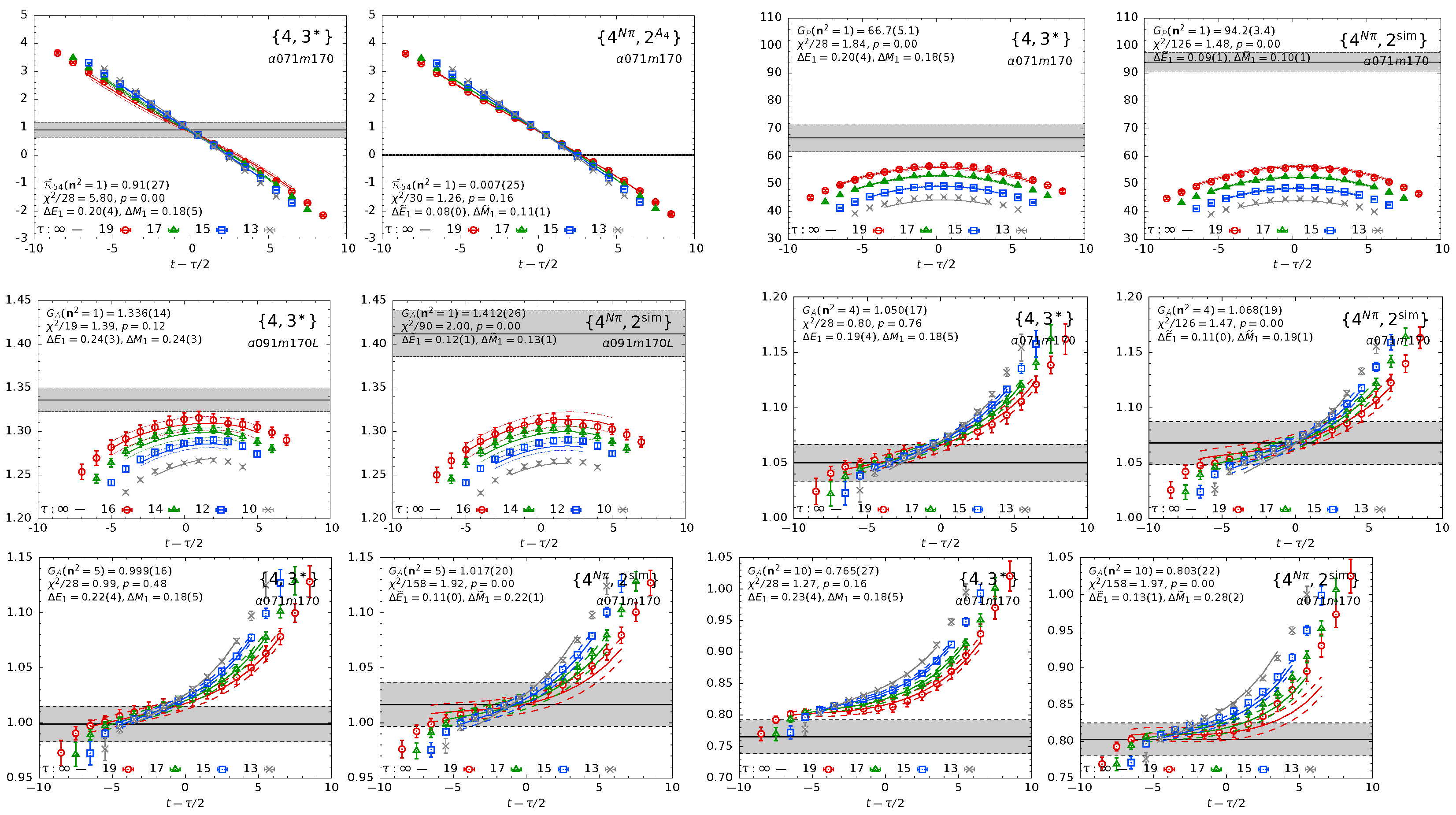
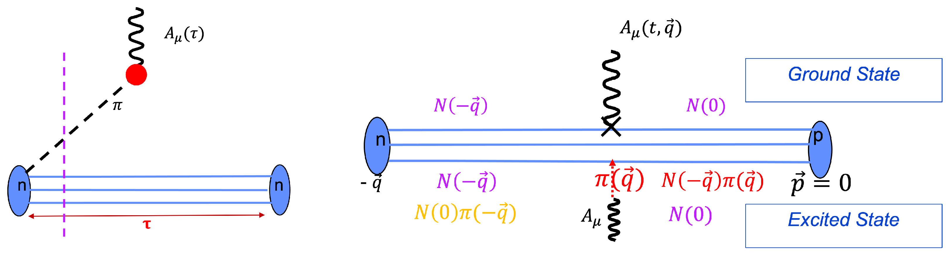
It turned out that two-state fits to provided a data-driven method [38] that exposed these states and confirmed that the lowest of the tower of states makes a very significant contribution. By itself, is dominated by excited states and fits to it using the from , which gave very poor . Making fits leaving a free parameter dramatically improved the (compare left two panels in top row of Figure 2), and the resulting output values of on either side of operator insertion were roughly consistent with as shown in Figure 3 (reproduced from Ref. [38]). An illustration of the current understanding of the transitions contributing to the GSME and of the lowest-contributing excited states is shown in Figure 4 (right).
The fact that there is an enhancement of the ME in the axial channel has been understood for over 60 years as the “pion pole dominance” (PPD) hypothesis. On the lattice, the creation of a state by is suppressed by the 3D volume compared to just the nucleon, as each state has a normalization factor of for a point (local) source . The axial current can, however, couple to this pion, and because the pion is light, this coupling can occur anywhere in the time slice at which the current is inserted with momentum (see Figure 4 (left)). This gives a factor of V enhancement, thus approximately canceling the normalization factor [36,37]. Thus, the ME obtains an enhanced contribution that is an artifact to be removed when the the pion comes on shell. Note that since energy is not conserved on the lattice, both the neutron and the pion can come on shell, however, since momentum is conserved, and possible excited states must have the same total momentum as the neutron state. PPD tells us that the axial current with momentum can be viewed as the insertion of a pion with , and this has a large coupling to the nucleon. These processes are illustrated in Figure 4.
Having identified large contributions from the state, certainly in the extraction of and , the question is—do we need to include other multihadron and radial excited state contributions if we want results with percent level precision? What about in ? Note that, in addition to the enhanced contribution shown in Figure 4, PT also indicates that the one-loop contributions due to the diagram shown in Figure 5 (again a contribution) could be in all the five . Thus, the state could be significant for extracting (the GSME ) from at the percent precision desired. Based on these arguments, it is clear that one needs at least three-state fits to the five in Equation (3)—the ground state, the state, and one other that effectively accounts for all other excited state contributions.
The caption of Figure 2 points out some of the features of the ESC observed in current data and the efficacy of fits to the spectral decomposition of with and without including the lowest state to remove the ESC.
In my evaluation, the details of the fits made to remove ESC are the most significant differences between the calculations performed by the different collaborations. With the current methodology, higher statistics data are needed to improve these fits and reduce the dependence on exactly how the analyses are done.
A very important point to keep in mind is that fit parameters in a truncated ansatz (the and in say a three-state fit in our case) try to incorporate the effects of all contributions. Thus, the connection between parameters coming out of fits to a truncated Equation (3) and physical states made in Figure 3 and Figure 4 are very approximate at best.
2.4. Satisfying PCAC
The nonsinglet PCAC relation between the bare axial, , and pseudoscalar, , currents is the following:
where the quark mass parameter includes all the renormalization factors, and is the light quark mass in the isospin symmetric limit. Using the decomposition in Equations (4) and (5) of the GSME, the PCAC relation requires that the three form factors , , and must satisfy on each ensemble up to discretization errors; thus, the relation is
All prior Ref. [35] calculations did not check this relation and missed observing that the data showed large deviations. Calculations subsequent to Ref. [38] that include the lowest mass gap state in the analysis obtain form factors that already satisfy the PCAC to within ≈10% at a lattice spacing of fm. (The ETMC result is an exception, as explained in Ref. [23] ). An illustration of the size of the deviation from unity of , without and with the lowest state included, is shown in Figure 6 taken from Ref. [19].
To summarize, satisfying the PCAC relation in Equation (12) provides a strong and necessary constraint on the extraction of the three axial form factors. PT analysis by Bär [36,37] and data-driven validation in Refs. [29,30,38] show that the lowest state makes a large contribution and needs to be included in the analysis. For percent level precision, the next question is—what other states need to be included? Current analyses include up to three states, where the third state, if the parameters are left free, is effectively trying to account for all of the residual ESC. Such fits have been implemented in different ways. For example, in Ref. [29], the state is hardwired, and the third state is taken to be the lowest excited state in fits to . In Refs. [19,27,38], a simultaneous fit to all five and P correlators is made wherein the correlator fixes to being close to the state. Over time, with much higher statistics data, results from various methods and collaborations should converge.
2.5. Extrapolating Lattice AVFF to The Physical Point for Use in Phenomenology
The next step, once ESC have been removed and form factors have been extracted from GSME on a given ensemble, is to extrapolate these data to the physical point to provide a parameterized form for and that can be used in phenomenology. The challenge is that the discrete set of values at which the data are obtained are different on each ensemble.
One simple way to implement this consists of the following three steps:
- Parameterize the data on each ensemble. Depending on the number of values, it could be a suitably truncated z expansion or a Padé. The expected asymptotic behavior can be built in by using sum rules in the z expansion [39] or through an Padé in . The Mainz collaboration [26] combines the removal of the ESC at various values of and the parameterization on a given ensemble to include correlations.
- Pick n values, , over a range of say GeV2. Extrapolate the data at each of these values of using a simultaneous fit in } to the physical point. (Note that I use or to define the light quark mass interchangeably.) A typical ansatz used for such chiral continuum finite volume (CCFV) extrapolations iswhere I have kept only the lowest order corrections in each of the variables and assumed that discretization errors start at .
- Having obtained the form factor in the continuum limit at points with , carry out the final parameterization again using a truncated z expansion or a Padé.
This three-step process can be done within a single bootstrap procedure to propagate errors as has been done in Refs. [19,27] to produce the NME and PNDME results shown in Figure 7. Or, these steps can be combined, especially if there are correlations between them. For example, as can be done in step (ii) to account for correlations between the coefficients of the CCFV fits for different values of .
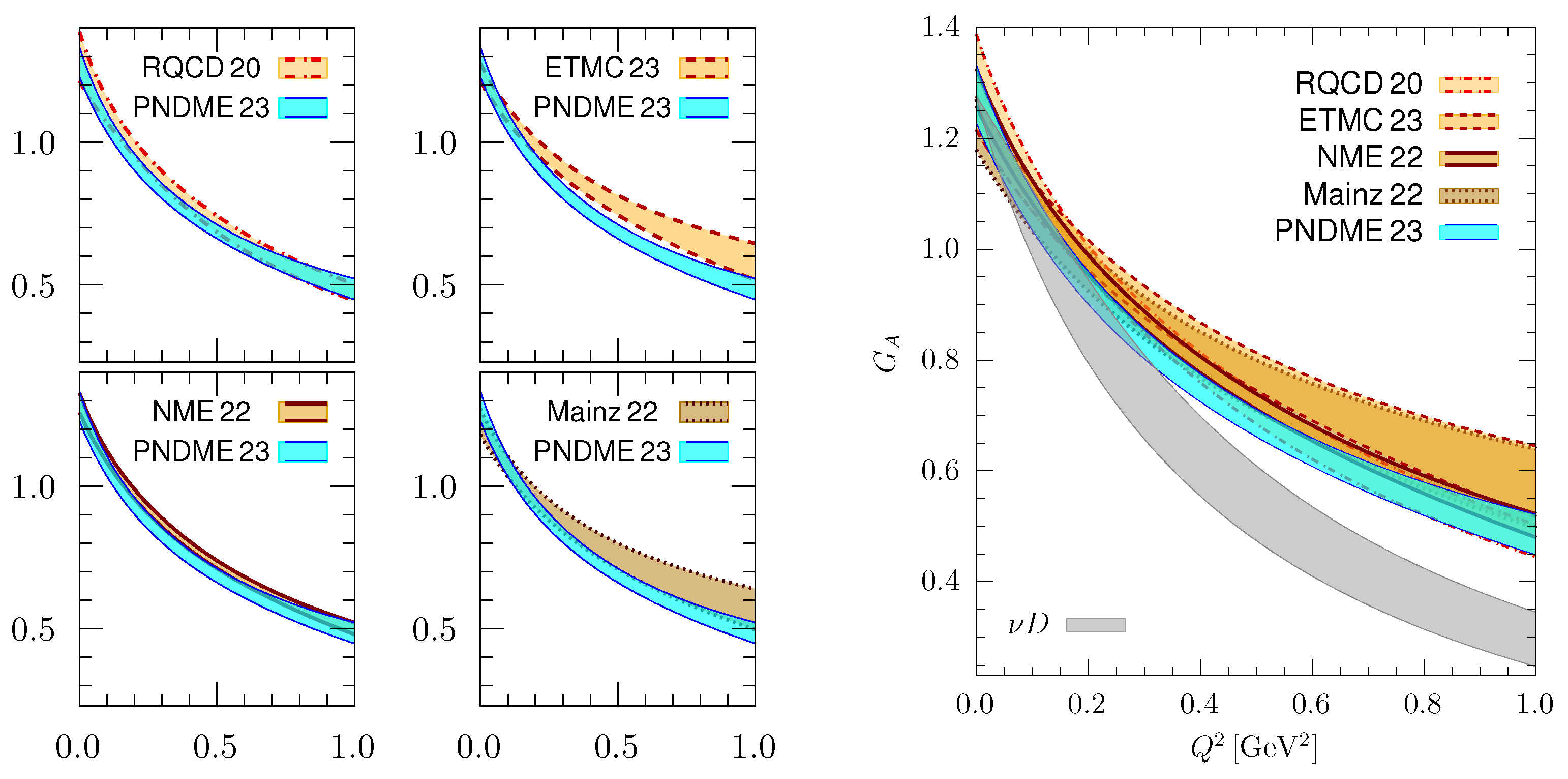
The plots in Figure 7 provide two comparisons. In the panels on the left, the physical point results from the RQCD [24,29], ETMC [23], NME [27], and Mainz [26] collaborations are compared against those from the PNDME [19]. On the right, they are overlaid and compared to the phenomenological extraction from the old neutrino–deuterium bubble chamber data [20]. The PNDME, RQCD, and NME data mostly overlap, whereas the ETMC and Mainz data overlap and fall off slower for GeV2. On the other hand, the neutrino–deuterium (D) data [20] fall off much faster for GeV2. Overall, as shown in the right plot, the five lattice QCD estimates are consistent within and lie about above the D band for GeV2.
There also are results from the CalLAT [16], PACS [25,40], and LHP+RBC+UKQCD [41] collaborations, which have not been included in the comparison because they have not been extrapolated to the physical point. The Fermilab collaboration [31] has embarked on the much harder problem of calculating transition matrix elements as well, e.g., or .
From the analysis of the NME and PNDME data, my understanding is that the differences in exactly how the ESC values are handled by the various collaborations and the uncertainty in the final results should be considered as a work in progress. The uncertainty from the differences in the overall procedure for parameterization and CCFV extrapolation is, I believe, smaller, especially since the data do not show a large dependence on any of the three parameters , especially for fm and , as illustrated in Figure 8 [19,27]. Hopefully, the next generation calculations will shed light on and possibly resolve the various differences.
Other findings in Refs. [19,27] are that (i) the dipole ansatz gives poor fits (very low p values) to data on many ensembles. My conclusion, therefore, is that the lattice data already show that the dipole ansatz does not have enough parameters to capture the behavior over the range GeV2. The second finding is that (ii) The PPD relation between and works very well.
2.6. Consistency Check in the Extraction of the Axial Charge
There are two ways in which one can extract the axial charge . The first is from the forward matrix element using in Equation (8) with , and the second is by extrapolating the form factor to . I am considering them as separate because the extraction from the forward matrix element is computationally clean: has the smallest errors, and the verification of the symmetry of the data about is a good test. The errors grow with , as shown in Figure 2. On the other hand, is constrained by being part of the PCAC relation, Equation (12), that has to be satisfied. The two results must agree after CCFV extrapolation. Based on the data in Ref. [19], I conclude the following:
- The difference between extracted without and with including states is , i.e., on including one (the lowest) state in the analysis. Note that the errors in each result are .
- The difference between extracted by extrapolating data obtained without and with including the lowest state is also , i.e., . Again, the errors in each are .
- Thus, for each of the two cases, without and with including states, we obtain consistent estimates for the charge from the two methods; however, the results including the state are about larger. This difference is consistent with the expected one-loop correction to the charge in PT; however, it is roughly a one combined effect and, therefore, needs validation. My pick for the final result is the analysis including the state, since it gives form factors that satisfy the PCAC relation. Higher precision data are needed to further clarify the other significant ESCs and how to include them.
3. Comparison of Charges Obtained by Various Lattice Collaborations
The results for the axial charge, , the charge radius squared, , the induced pseudoscalar coupling , and the pion–nucleon coupling extracted from and by various collaborations using the relations result in the following:
which are summarized in Table 1. Here, is the muon mass, is the energy scale of muon capture, and MeV is the pion decay constant.
The results show about variation in , , and and about in . Part of this is likely due to different methodologies used in the analysis, in particular how and if the lowest state is included in the analysis. These results will improve over time.
4. Comparison of the Differential Cross-Section Using Lattice AVFF with MINERA Data
A comparison of the antineutrino–nucleon charged current elastic cross sections calculated using predictions of AVFF from lattice (PNDME 23 [19]) and neutrino–deuterium analysis [20] with MINERvA measurement [17,42] is presented in Figure 9, which is reproduced from Ref. [18]. A test was performed to determine the significance of the differences between the three. No significant difference was found between MINERvA–lattice QCD (PNDME) and between MINERvA–deuterium results. A tension was, however, found between the PNDME and the deuterium results. Based on data shown in Figure 7, the deviation in the deuterium–Mainz and deuterium–ETMC will be even larger. To assess the scope for future progress, three regions of with different prospects for the extraction of AVFF from lattice QCD and MINERvA-like experiments were identified.
For , LQCD predictions and fits to the deuterium bubble chamber data are in good agreement. In this region, the experimental errors in the measurement on hydrogen by MINERvA are large, whereas the errors in the parameterization of the deuterium bubble chamber data are smaller. The D result has often been used as a benchmark; however, note that there is unresolved uncertainty in the deuterium data as discussed in Ref. [20]. Also, no new deuterium data are expected in the near-term, so I do not comment on its future prospects. Lattice QCD data are competitive and will improve steadily. This region will be well characterized by the axial charge, the axial charge radius, and well parameterized by a low-order z expansion or a Padé.
For , the AVFF from PNDME has the smallest errors, and the predicted differential cross-section lies above the hydrogen and D values, i.e., the same ordering as for the AVFF shown in Figure 9 (left). Future improvements in both the hydrogen data and lattice calculations will provide robust crosschecks in this region.
The region is where lattice QCD data, even with current methodology, will improve rapidly as more simulations are done closer to MeV, and on larger volumes, because on a given ensemble and for given statistics, the value of with a good signal (usually specified by the lattice momentum ) decreases in these limits.
For , current LQCD data have large statistical errors and systematic uncertainties—these are discretization and residual excited state contributions. With the current methodology, the lattice AVFF comes mostly from simulations with MeV [19]. New methods are needed to obtain data from simulations with physical pion masses, MeV. Similarly, improvements further MINERvA and follow-up experiments are needed to cover the full range of relevant for DUNE.
5. Concluding Remarks
Extensive calculations of the AVFF are being carried out by at least the following nine lattice QCD collaborations: PNDME [19], RQCD [24,29], ETMC [23], NME [27], Mainz [26], CalLAT [16], PACS [25,40], LHP+RBC+UKQCD [41], and Fermilab [31]. As shown in Section 3 and Section 2.5, we now have results to within 10% precision. The major of the uncertainty comes from resolving and removing excited state contributions.
The good news is that the methodology for the calculation of the correlation functions, and , is robust. The bad news is that the exponentially falling signal-to-noise ratio in them means that ESC are large at source–sink separations possible in today’s calculations. Second, it is also clear that multihadron, , excited states give large contributions and must be included in the analysis to remove them. Unfortunately, it is not yet known how many of these states will need to be included in the analysis for percent level precision. The operator constraint that the form factors satisfy the PCAC relation in Equation (12) provides a valuable check that must be carried out in all calculations. The third challenge is obtaining data at large , because the discretization and statistical errors grow with on a given ensemble, and the , i.e., the lattice momenta with the largest that has a good signal-to-noise ratio, decreases as simulations are done closer to the physical point. Thus, to obtain data for GeV2 on physical pion mass ensembles will need/benefit from new methodology.
I estimate that a factor of ten increase in statistics will reduce the statistical errors to a level that will provide much more clarity in removing the ESC. Similary new developments, including variational methods [30] with multihadron states and momentum smearing [43], will improve the calculations and extend the range of . I anticipate improvements in both statistics and methods will provide LQCD predictions of AVFF for nucleons in the range (hopefully higher) with percent level precision by about 2030 in concert with DUNE producing data.
Funding
R. Gupta was partly supported by the U.S. Department of Energy, Office of Science, Office of High Energy Physics under Contract No. DE-AC52-06NA25396 and by the LANL LDRD program.
Data Availability Statement
This is a review article and no new data were generated. All data quoted are referenced to original published papers.
Acknowledgments
Many thanks to my collaborators, Yong-Chull Jang, Sungwoo Park, Oleksandr Tomalak, Tanmoy Bhattacharya, Vincenzo Cirigliano, Huey-Wen Lin, Emanuele Mereghetti, Santanu Mondal, and Boram Yoon for making the PNDME and NME results happen. Also to all who presented relevant results at Lattice 2023. The PNDME and NME calculations used the Chroma software suite [44] and resources at (i) the National Energy Research Scientific Computing Center, a DOE Office of Science User Facility supported by the Office of Science of the U.S. Department of Energy under Contract No. DE-AC02-05CH11231; (ii) the Oak Ridge Leadership Computing Facility, which is a DOE Office of Science User Facility supported under Contract DE-AC05-00OR22725, through awards under the ALCC program project LGT107 and INCITE award HEP133; (iii) the USQCD collaboration, which is funded by the Office of Science of the U.S. Department of Energy; and (iv) Institutional Computing at Los Alamos National Laboratory.
Conflicts of Interest
The author declares no conflicts of interest. The funders had no role in the design of the study; in the collection, analyses, or interpretation of data; in the writing of the manuscript; or in the decision to publish the results.
References
- Mendenhall, M.; Pattie, R.W., Jr.; Bagdasarova, Y.; Berguno, D.B.; Broussard, L.J.; Carr, R.; UCNA Collaboration. Precision measurement of the neutron β-decay asymmetry. Phys. Rev. 2013, C87, 032501. [Google Scholar] [CrossRef]
- Brown, M.A.P.; Dees, E.B.; Adamek, E.; Allgeier, B.; Blatnik, M.; Bowles, T.J.; UCNA Collaboration. New result for the neutron β-asymmetry parameter A0 from UCNA. Phys. Rev. 2018, C97, 035505. [Google Scholar] [CrossRef]
- Märkisch, B.; Mest, H.; Saul, H.; Wang, X.; Abele, H.; Dubbers, D.; Klopf, M.; Petoukhov, A.; Roick, C.; Soldner, T.; et al. Measurement of the Weak Axial-Vector Coupling Constant in the Decay of Free Neutrons Using a Pulsed Cold Neutron Beam. Phys. Rev. Lett. 2019, 122, 242501. [Google Scholar] [CrossRef] [PubMed]
- Mund, D.; Maerkisch, B.; Deissenroth, M.; Krempel, J.; Schumann, M.; Abele, H.; Petoukhov, A.; Soldner, T. Determination of the Weak Axial Vector Coupling from a Measurement of the Beta-Asymmetry Parameter A in Neutron Beta Decay. Phys. Rev. Lett. 2013, 110, 172502. [Google Scholar] [CrossRef] [PubMed]
- Ademollo, M.; Gatto, R. Nonrenormalization Theorem for the Strangeness Violating Vector Currents. Phys. Rev. Lett. 1964, 13, 264–265. [Google Scholar] [CrossRef]
- Donoghue, J.F.; Wyler, D. Isospin breaking and the precise determination of Vud. Phys. Lett. 1990, B241, 243. [Google Scholar] [CrossRef]
- Bhattacharya, T.; Cirigliano, V.; Cohen, S.D.; Filipuzzi, A.; Gonzalez-Alonso, M.; Graesser, M.L.; Gupta, R.; Lin, H.W. Probing Novel Scalar and Tensor Interactions from (Ultra)Cold Neutrons to the LHC. Phys. Rev. D 2012, 85, 054512. [Google Scholar] [CrossRef]
- Ivanov, A.N.; Pitschmann, M.; Troitskaya, N.I.; Berdnikov, Y.A. Bound-state β-decay of the neutron re-examined. Phys. Rev. C 2014, 89, 055502. [Google Scholar] [CrossRef]
- Czarnecki, A.; Marciano, W.J.; Sirlin, A. Neutron Lifetime and Axial Coupling Connection. Phys. Rev. Lett. 2018, 120, 202002. [Google Scholar] [CrossRef] [PubMed]
- Czarnecki, A.; Marciano, W.J.; Sirlin, A. Radiative Corrections to Neutron and Nuclear Beta Decays Revisited. Phys. Rev. 2019, D100, 073008. [Google Scholar] [CrossRef]
- Czarnecki, A.; Marciano, W.J.; Sirlin, A. Pion beta decay and Cabibbo-Kobayashi-Maskawa unitarity. Phys. Rev. 2020, D101, 091301. [Google Scholar] [CrossRef]
- Horoi, M.; Neacsu, A. Shell model study of using an effective field theory for disentangling several contributions to neutrinoless double-β decay. Phys. Rev. C 2018, 98, 035502. [Google Scholar] [CrossRef]
- Carroll, B.W.; Ostlie, D.A. An Introduction to Modern Astrophysics, 2nd ed.; Pearson Addison-Wesley: Boston, MA, USA, 2007. [Google Scholar]
- Ruso, L.A.; Ankowski, A.M.; Bacca, S.; Balantekin, A.B.; Carlson, J.; Gardiner, S.; Gonzalez-Jimenez, R.; Gupta, R.; Hobbs, T.J.; Hoferichter, J.M.; et al. Theoretical tools for neutrino scattering: Interplay between lattice QCD, EFTs, nuclear physics, phenomenology, and neutrino event generators. arXiv 2022, arXiv:2203.09030. [Google Scholar]
- Kronfeld, A.S.; Richards, D.G.; Detmold, W.; Gupta, R.; Lin, H.W.; Liu, K.F.; Meyer, A.S.; Sufian, R.; Syritsyn, S. Lattice QCD and Neutrino-Nucleus Scattering. Eur. Phys. J. 2019, A55, 196. [Google Scholar] [CrossRef]
- Meyer, A.S.; Walker-Loud, A.; Wilkinson, C. Status of Lattice QCD Determination of Nucleon Form Factors and their Relevance for the Few-GeV Neutrino Program. 2022. Available online: https://www.annualreviews.org/doi/abs/10.1146/annurev-nucl-010622-120608 (accessed on 1 October 2023).
- Cai, T.; Moore, M.L.; Olivier, A.; Akhter, S.; Dar, Z.A.; Ansari, V.; Ascencio, M.V.; Bashyal, A.; Bercellie, A.; Betancourt, M. Measurement of the axial vector form factor from antineutrino–proton scattering. Nature 2023, 614, 48–53. [Google Scholar] [CrossRef] [PubMed]
- Tomalak, O.; Gupta, R.; Bhattacharya, T. Confronting the axial-vector form factor from lattice QCD with MINERvA antineutrino-proton data. Phys. Rev. D 2023, 108, 074514. [Google Scholar] [CrossRef]
- Jang, Y.C.; Gupta, R.; Bhattacharya, T.; Yoon, B.; Lin, H.W. Nucleon Isovector Axial Form Factors. arXiv 2023, arXiv:2305.11330. [Google Scholar] [CrossRef]
- Meyer, A.S.; Betancourt, M.; Gran, R.; Hill, R.J. Deuterium target data for precision neutrino-nucleus cross sections. Phys. Rev. D 2016, 93, 113015. [Google Scholar] [CrossRef]
- Aoki, Y.; Blum, T.; Colangelo, G.; Collins, S.; Morte, M.D.; Dimopoulos, P.; Dürr, S.; Feng, X.; Fukaya, H.; Golterman, M.; et al. FLAG Review 2021. Eur. Phys. J. C 2022, 82, 869. [Google Scholar] [CrossRef]
- Aoki, S.; Aoki, Y.; Bečirević, D.; Blum, T.; Colangelo, G.; Collins, S.; Della, M.; Dimopoulos, P.; Dürr, S.; Fukaya, H.; et al. FLAG Review 2019: Flavour Lattice Averaging Group (FLAG). Eur. Phys. J. C 2020, 80, 113. [Google Scholar] [CrossRef]
- Alexandrou, C.; Bacchio, S.; Constantinou, M.; Finkenrath, J.; Frezzotti, R.; Kostrzewa, B.; Koutsou, G.; Spanoudes, G.; Urbach, C. Nucleon axial and pseudoscalar form factors using twisted-mass fermion ensembles at the physical point. arXiv 2023, arXiv:2309.05774. [Google Scholar] [CrossRef]
- Bali, G.S.; Collins, S.; Heybrock, S.; Löffler, M.; Rödl, R.; Söldner, W.; Weishäupl, S. Octet baryon isovector charges from Nf=2+1 lattice QCD. arXiv 2023, arXiv:2305.04717. [Google Scholar] [CrossRef]
- Tsuji, R.; Tsukamoto, N.; Aoki, Y.; Ishikawa, K.I.; Kuramashi, Y.; Sasaki, S.; Shintani, E.; Yamazaki, T. Nucleon isovector couplings in Nf = 2+1 lattice QCD at the physical point. Phys. Rev. D 2022, 106, 094505. [Google Scholar] [CrossRef]
- Djukanovic, D.; von Hippel, G.; Koponen, J.; Meyer, H.B.; Ottnad, K.; Schulz, T.; Wittig, H. Isovector axial form factor of the nucleon from lattice QCD. Phys. Rev. D 2022, 106, 074503. [Google Scholar] [CrossRef]
- Park, S.; Gupta, R.; Yoon, B.; Mondal, S.; Bhattacharya, T.; Jang, Y.C.; Joó, B.; Winter, F. Precision nucleon charges and form factors using (2+1)-flavor lattice QCD. Phys. Rev. D 2022, 105, 054505. [Google Scholar] [CrossRef]
- Alexandrou, C.; Bacchio, S.; Constantinou, M.; Dimopoulos, P.; Finkenrath, J.; Hadjiyiannakou, K.; Jansen, K.; Koutsou, G.; Kostrzewa, B.; Leontiou, T.; et al. Nucleon axial and pseudoscalar form factors from lattice QCD at the physical point. Phys. Rev. D 2021, 103, 034509. [Google Scholar] [CrossRef]
- Bali, G.S.; Barca, L.; Collins, S.; Gruber, M.; Löffler, M.; Schäfer, A.; Söldner, W.; Wein, P.; Weishäupl, S.; Wurm, T. Nucleon axial structure from lattice QCD. J. High Energy Phys. 2020, 5, 126. [Google Scholar] [CrossRef]
- Barca, L.; Bali, G.; Collins, S. Toward N to Nπ matrix elements from lattice QCD. Phys. Rev. D 2023, 107, L051505. [Google Scholar] [CrossRef]
- Grebe, A.V.; Wagman, M. Nucleon-Pion Spectroscopy from Sparsened Correlators. arXiv 2023, arXiv:2312.00321. [Google Scholar]
- Gusken, S.; Low, U.; Mutter, K.H.; Sommer, R.; Patel, A.; Schilling, K. Nonsinglet Axial Vector Couplings of the Baryon Octet in Lattice QCD. Phys. Lett. B 1989, 227, 266–269. [Google Scholar] [CrossRef]
- Parisi, G. The Strategy for Computing the Hadronic Mass Spectrum. Phys. Rept. 1984, 103, 203–211. [Google Scholar] [CrossRef]
- Lepage, G.P. The Analysis of Algorithms for Lattice Field Theory. Boulder TASI 1989, 97–120. [Google Scholar] [CrossRef]
- Gupta, R.; Jang, Y.C.; Lin, H.W.; Yoon, B.; Bhattacharya, T. Axial Vector Form Factors of the Nucleon from Lattice QCD. Phys. Rev. 2017, D96, 114503. [Google Scholar] [CrossRef]
- Bär, O. Nucleon-pion-state contamination in lattice calculations of the axial form factors of the nucleon. In Proceedings of the 36th International Symposium on Lattice Field Theory (Lattice 2018), East Lansing, MI, USA, 22–28 July 2018. [Google Scholar]
- Bär, O. Nπ-state contamination in lattice calculations of the nucleon axial form factors. Phys. Rev. D 2019, 99, 054506. [Google Scholar] [CrossRef]
- Jang, Y.C.; Gupta, R.; Yoon, B.; Bhattacharya, T. Axial Vector Form Factors from Lattice QCD that Satisfy the PCAC Relation. Phys. Rev. Lett. 2020, 124, 072002. [Google Scholar] [CrossRef] [PubMed]
- Lee, G.; Arrington, J.R.; Hill, R.J. Extraction of the proton radius from electron-proton scattering data. Phys. Rev. D 2015, 92, 013013. [Google Scholar] [CrossRef]
- Tsuji, R.; Aoki, Y.; Ishikawa, K.I.; Kuramashi, Y.; Sasaki, S.; Sato, K.; Shintani, E.; Watanabe, H.; Yamazaki, T. Nucleon form factors in Nf = 2+1 lattice QCD at the physical point: Finite lattice spacing effect on the root-mean-square radii. arXiv 2023, arXiv:2311.10345. [Google Scholar]
- Ohta, S. Nucleon isovector form factors from domain-wall lattice QCD at the physical mass. arXiv 2023, arXiv:2311.05894. [Google Scholar]
- Irani, F.; Goharipour, M.; Hashamipour, H.; Azizi, K. New insight on the nucleon structure from recent MINERvA measurement of the antineutrino-proton scattering cross-section. arXiv 2023, arXiv:2306.13060. [Google Scholar]
- Bali, G.S.; Lang, B.; Musch, B.U.; Schäfer, A. Novel quark smearing for hadrons with high momenta in lattice QCD. Phys. Rev. D 2016, 93, 094515. [Google Scholar] [CrossRef]
- Edwards, R.G.; Joo, B. The Chroma software system for lattice QCD. Nucl.Phys.Proc.Suppl. 2005, 140, 832. [Google Scholar] [CrossRef]
Figure 1.
Quark line diagrams for the gauge-invariant time-ordered correlation functions and . The gluon lines are shown to indicate that all possible gluon exchanges between quarks are included, i.e., it is a fully nonperturbative calculation. The electromagnetic and axial form factors are calculated by inserting the vector, , and axial, , currents with momentum at times t in between the nucleon source and sink separated by time .

Figure 2.
Data for the ratio that, in the limits and , should be independent of and t, i.e., lie on a horizontal line in the center about with value that is the GSME. Current data show large ESC, and the gray band is the estimate of the GSME given by the fit to Equation (3). In each row, the data in each pair of panels are the same, but the fit on the left is without the state and on the right is with the state. The top row (panels 1 and 2) show the data and fit to with . These two panels illustrate (i) the improvement () in the fit to data with the inclusion of the state and (ii) a very large ESC indicated by the large slope slowly rotating counterclockwise to the expected horizontal band. The right two panels show the data and fits to with that should give . These two panels illustrate that the difference in the without and with including the state is about (enhanced ESC), and the is better with the state. The panels in rows two and three show the data and fit to with , that should give the for . These pairs of panels illustrate that the difference in the without and with including the state is a few percent, and the of the two fits is comparable. Note the change in the behavior: the data converge from below, while for (1,1,1) and higher momenta the data are rotating clockwise to the expected horizontal line, and the fits become less robust with . See Ref. [27] for details on the data and the fits.

Figure 3.
Results for the energy gaps () for the first excited state extracted from fits to the correlator labeled and . These mass gaps are compared with the first excited state energy from four-state fits to the nucleon two-point correlator (black circles). Note that the difference between them (black circles versus blue triangles), and consequently the difference between the form factors extracted increases as MeV and (equivalently ).

Figure 4.
The quark line diagrams illustrating the contribution of states. (Left) the current annihilates the pion produced by the source. (Right) The states involved in the transitions: the ground state process is shown above the quark line diagram, and that involving an excited state on one side of the current insertion is shown below.

Figure 5.
The one-loop correction to the three-point function.

Figure 6.
(Left) Results for on 10 ensembles from fits to without including the state, i.e., the spectrum taken from fits to . (Right) Including the state. For PCAC to be satisfied, should express unity up to discretization errors. The dotted lines show the 5% deviation band.
Figure 6.
(Left) Results for on 10 ensembles from fits to without including the state, i.e., the spectrum taken from fits to . (Right) Including the state. For PCAC to be satisfied, should express unity up to discretization errors. The dotted lines show the 5% deviation band.

Figure 7.
(Left) Comparison of the nucleon axial vector form factor as a function of , the momentum transfer squared, obtained by the (i) PNDME 23 [19] shown by the turquoise band; (ii) RQCD 19 [29] (light faun band); ETMC 21 [23] (faun band); NME 22 [27] (light brown band); and Mainz 22 [26] (brown band). (Right) These five lattice results for are shown together along with the D band which is the fit to the deuterium data given in Ref. [20].

Figure 8.
The data for renormalized on 13 HISQ ensembles show small variations in . The data are statistics limited. Figure reproduced from Ref. [19].
Figure 8.
The data for renormalized on 13 HISQ ensembles show small variations in . The data are statistics limited. Figure reproduced from Ref. [19].

Figure 9.
(Left) Comparison of the parameterized nucleon axial vector form factor versus up to 2 GeV2 obtained from (i) fit to the deuterium bubble-chamber data [20] shown by blue solid lines with error band; (ii) fit to recent MINERvA antineutrino–hydrogen data [17], shown by black dashed lines and turquoise error band; and (iii) lattice QCD result obtained by the PNDME Collaboration [19] shown by red solid lines without a band. (Right) A comparison of antineutrino–nucleon charged current elastic differential cross section using AFF from (i) lattice QCD by the PNDME collaboration [19] (red bands) and (ii) the deuterium bubble-chamber data [20] (black bands) with the MINERvA antineutrino–hydrogen data [17] (black circles). These figures are taken from Ref. [18].


Table 1.
Comparison of , , , and from recent calculations: PNDME 23 [19], RQCD [24,29], ETMC [28], PACS [25,40], Mainz [26], and NME [27]. Results for are in the scheme at scale 2 GeV. Earlier results for have been reviewed in the FLAG reports [21,22].
| Collaboration | fm2 | |||
|---|---|---|---|---|
| PNDME 23 | 1.292(53)(24) | 0.439(56)(34) | 9.03(47)(42) | 14.14(81)(85) |
| RQCD 19/23 | 0.449(88) | 8.68(45) | 12.93(80) | |
| ETMC 23 | 1.283(22) | 0.339(46)(6) | 8.99(39)(49) | 13.25(67)(69) |
| PACS 23 | 1.264(14)(1) | 0.316(67) | ||
| Mainz 22 | 1.225(39)(25) | 0.370(63)(16) | ||
| NME 21 | 1.32(6)(5) | 0.428(53)(30) | 7.9(7)(9) | 12.4.(1.2) |
Disclaimer/Publisher’s Note: The statements, opinions and data contained in all publications are solely those of the individual author(s) and contributor(s) and not of MDPI and/or the editor(s). MDPI and/or the editor(s) disclaim responsibility for any injury to people or property resulting from any ideas, methods, instructions or products referred to in the content. |
© 2024 by the author. Licensee MDPI, Basel, Switzerland. This article is an open access article distributed under the terms and conditions of the Creative Commons Attribution (CC BY) license (https://creativecommons.org/licenses/by/4.0/).
Share and Cite
MDPI and ACS Style
Gupta, R. Isovector Axial Charge and Form Factors of Nucleons from Lattice QCD. Universe 2024, 10, 135. https://doi.org/10.3390/universe10030135
AMA Style
Gupta R. Isovector Axial Charge and Form Factors of Nucleons from Lattice QCD. Universe. 2024; 10(3):135. https://doi.org/10.3390/universe10030135
Chicago/Turabian StyleGupta, Rajan. 2024. "Isovector Axial Charge and Form Factors of Nucleons from Lattice QCD" Universe 10, no. 3: 135. https://doi.org/10.3390/universe10030135
Note that from the first issue of 2016, this journal uses article numbers instead of page numbers. See further details here.