Classification of Planetary Motion around Super-Jupiters and Brown Dwarfs

Abstract

We investigate the orbital dynamics of an exosystem consisting of a solar-mass host star, a transiting body, and an Earth-size exoplanet within the framework of the generalized three-body problem. Depending on its mass, the transiting body can either be a super-Jupiter or a brown dwarf. To determine the final states of the Earth-size exoplanet, we conduct a systematic and detailed classification of the available phase space trajectories. Our classification scheme distinguishes between the bounded, escape, and collisional motions of the Earth-size exoplanet. Additionally, for cases of ordered (regular) motion, we further categorize the associated initial conditions based on the geometry of their respective trajectories. These bounded regular trajectories hold significant importance as they provide insights into the regions of phase space where the motion of the Earth-size exoplanet can be dynamically stable. Of particular interest is the identification of initial conditions that result in a bounded exomoon-like orbit of the Earth-size exoplanet around the transiting body.

1. Introduction

Among the myriad configurations of exoplanetary systems, those involving a host star with a solar mass, a transiting body, and an exoplanet of Earth’s size hold particular significance due to their potential implications for habitability and the existence of exomoons. Previous statistical analyses of large samples of planetary candidates detected by the Kepler spacecraft suggested that a significant percentage of stars in the Milky Way galaxy may host planets ranging from 0.8 to 1.25 times the size of Earth and orbiting within the habitable zone [1]. The Kepler mission, along with its successors, the extended Kepler (K2) and the Transiting Exoplanet Survey Satellite (TESS), and in combination with various ground-based facilities has provided a vast amount of data not only on the mass, size, and orbital parameters of exosystems but also on the composition of the celestial objects involved (see, e.g., [2,3,4,5]). Additional data are foreseen to be obtained by the James Webb Space Telescope (JWST) in the near to mid-term future [6].

Despite the substantial progress that has been made in characterizing exoplanets and their host stars [7,8,9], a less explored field of exosystem studies lies in understanding the complex interactions and outcomes resulting from the gravitational interplay between multiple celestial bodies. In the realm of orbital dynamics, several approaches using few-body problems have been employed to gain a deeper understanding of the underlying dynamics of exosystems.

For example, Domingos et al. [10] employed an analytical approach within the framework of the restricted three-body problem to unveil the dynamic properties of hypothetical companion satellites orbiting extrasolar planets. Antoniadou & Voyatzis [11], on the other hand, investigated the dynamics of coplanar two-planet exosystems with high eccentricities using the general three-body problem to understand the long-term stability of such configurations. Subsequently, Antoniadou & Voyatzis [12] utilized the general four-body problem to study families of periodic orbits in exosystems within specific regions of phase space.

Keplerian orbital solutions are widely recognized as a fundamental framework for studying exoplanetary systems. They provide crucial information regarding orbital parameters, mass estimation, detection methods, stability analysis, and predictions for future observations [13]. However, when examining few-body exoplanetary systems ($N\ge 3$), specifically those involving a star, a transiting body, and an exoplanet, certain circumstances may give rise to chaotic behavior. This chaos can lead to unpredictable but limited excursions in planetary orbits, resulting in significant increases in eccentricity as the system explores the full region of phase space governed by conservation laws. Additionally, close encounters between planets may occur, potentially resulting in collisions or ejections [14]. These studies hold substantial interest as they enable the exploration of long-term stability within exoplanetary systems from a theoretical standpoint.

Our study focuses on investigating the orbital dynamics of an exosystem consisting of a solar-mass host star, a transiting body (such as a gas giant or brown dwarf), and an Earth-sized exoplanet. We aim to explore the diverse outcomes resulting from the interactions among these celestial bodies and develop a systematic understanding of their final states by examining the generalized three-body problem applied to point-particles. To achieve this, we employ a comprehensive approach to classify trajectories, which systematically explores the available phase space. We categorize trajectories into bounded, escape, and collisional motion, revealing distinct patterns and identifying regions of interest associated with the dynamics of the Earth-sized exoplanet. Furthermore, within the realm of bounded regular motion, we further classify the corresponding initial conditions based on the geometry of the trajectories. This classification allows us to delineate phase space regions where the motion of the Earth-sized exoplanet can be dynamically stable.

The paper is organized as follows: In Section 2, we provide essential details about the mathematical model and parameters used to study an exosystem consisting of three main bodies: a solar-mass star, a transiting body (such as a super-Jupiter or brown dwarf), and an Earth-sized exoplanet. Section 3 presents the numerical methodology used to classify the dynamical behavior of the Earth-sized exoplanet, along with an additional classification of regular bounded trajectories. In Section 4, using color-coded basin diagrams, we perform an orbit classification in different types of exoplanetary systems based on the masses of the host star and the transiting Jupiter-sized body. Lastly, in Section 5, we provide a brief discussion of our findings, highlighting the most important discoveries from our survey.

2. Presentation of the System of Bodies

Our system consists of three primary bodies: a host star, a transiting celestial body, and an exoplanet. The host star, denoted as $m_1$, possesses a greater mass compared to the other two bodies, represented by $m_2$ and $m_3$. Utilizing a heliocentric reference frame is advantageous due to the host star’s higher mass. In this frame, the host star is positioned at the origin $O(0,0,0)$, while the transiting celestial body and the exoplanet are located at coordinates ${\overrightarrow{r}}_2$ and ${\overrightarrow{r}}_3$, respectively. Thus, the equation of motion for $m_2$ (the transiting body) relative to $m_1$ can be expressed as

$$\ddot{\overrightarrow{r_2}}=-G\left(m_1+m_2\right)\frac{{\overrightarrow{r}}_2}{|{\overrightarrow{r}}_2{|}^3}+G{m}_3\left(\frac{{\overrightarrow{r}}_3-{\overrightarrow{r}}_2}{|{\overrightarrow{r}}_3-{\overrightarrow{r}}_2{|}^3}-\frac{{\overrightarrow{r}}_3}{|{\overrightarrow{r}}_3{|}^3}\right),$$

(1)

while the equation of motion for $m_3$ (exoplanet) relative to $m_1$ (star) reads as

$$\ddot{\overrightarrow{r_3}}=-G\left(m_1+m_3\right)\frac{{\overrightarrow{r}}_3}{|{\overrightarrow{r}}_3{|}^3}+G{m}_2\left(\frac{{\overrightarrow{r}}_2-{\overrightarrow{r}}_3}{|{\overrightarrow{r}}_2-{\overrightarrow{r}}_3{|}^3}-\frac{{\overrightarrow{r}}_2}{|{\overrightarrow{r}}_2{|}^3}\right).$$

(2)

It is worth mentioning that Figure 1 and Figure 2, along with the accompanying textual descriptions, have been adapted from our previous publication [15] to elucidate essential aspects of the model under investigation. Importantly, while a similarity between the two works exists, it is crucial to recognize that the current study operates within a distinct context and places emphasis on different facets of the subject matter. As such, the reuse of certain materials from our prior work serves to enhance clarity and maintain continuity in the presentation of our research findings.

In the subsequent discussion, we provide a comprehensive description of the parameters for each primary body within the system. The host star possesses a mass denoted as $m_1$, equivalent to 1 solar mass, and shares the same radius as the Sun. The transiting celestial body orbits the star in a circular path with a radius of 0.05 astronomical units (AU), resulting in an orbital period of approximately 4 days. The mass of the transiting body, represented as $m_2$, ranges from 5 to 70 times the mass of Jupiter. Depending on the mass range, $m_2$ is classified as either a transiting super-Jupiter or a brown dwarf. The mass of the exoplanet, denoted as $m_3$, remains fixed at 1 Earth mass.

For the body with mass $m_2$, we assume a radius of 1 Jupiter radius based on the established relationship between mass and radii for known super-Jupiters. This choice is supported by Figure 3 from Laughlin [16], which illustrates the distribution of the masses and radii of known super-Jupiters obtained from the NASA Exoplanet Archive (Update: 21 April 2023) (https://exoplanetarchive.ipac.caltech.edu/ (accessed on 5 May 2023)). Additionally, previous studies such as that by Hatzes & Rauer [17] have emphasized a noteworthy feature in the mass–radius relationship, indicating a local maximum of around 1 $M_J$ for giant planets, with a subsequent diminishing trend observed for larger masses in the brown dwarf regime. This suggests a level of consistency in radius across these objects. Therefore, our decision to maintain a fixed radius across the mass range of 5–70 $M_J$ aligns with the broader understanding of this relationship.

Adopting a heliocentric frame of reference simplifies our computations, requiring only the initial position and velocity of bodies with masses $m_2$ and $m_3$, obtained from standard Keplerian orbital elements. In our calculations, we set the gravitational constant (G) as $G=k^2$, where $k=0.01720209895$ (rad/day). Consequently, length, mass, and time units are expressed in astronomical units (AU), solar masses, and days, respectively.

3. Computational Methodology

Considering that the primary body $m_1$ is located at the origin of coordinates, we perform numerical integration of the equations of motion for the primary bodies $m_2$ and $m_3$. We utilize the Bulirsch–Stoer method with double precision, as it is particularly well-suited for solving stiff ordinary differential equations (ODEs) [18]. The tolerance parameter for the numerical integration is set to ${10}^{-12}$ by monitoring the behavior of the conserved quantity (total energy) throughout the integration process. This choice is based on the fundamental concept of the Bulirsch–Stoer integrator, which estimates the local truncation error at each step and adjusts the step size accordingly. Importantly, the total energy remains approximately constant within an order of ${10}^{-13}$ in all cases.

On the other hand, taking into account the graphical representation concept using basins, we classify each trajectory’s initial condition by assigning a characteristic color based on its final state [19]. In the case of the exoplanet $m_3$, it can exhibit different types of orbits. Firstly, there is bounded regular motion, which describes the exoplanet orbiting the star and the transiting body predictably. Alternatively, there is bounded chaotic motion, where the exoplanet exhibits chaotic motion around the star and the transiting body. Additionally, collisions may occur between the exoplanet and either the star or the transiting body. Lastly, an escape orbit refers to the exoplanet overcoming the gravitational pull of the star and the transiting body, allowing it to move away indefinitely.

As a numerical tool that assists in classifying motion as either regular or chaotic, we utilize the SALI index (Smaller Alignment Index) [20]. The SALI index quantifies the alignment between two nearby trajectories evolving in the same dynamical system, providing a measure of how the separation between these trajectories changes over time. It offers valuable insights into the stability and predictability of the system (see, for instance, [21,22] for more details).

In the context of our current dynamical system, this index allows us to classify the motion of the Earth-size exoplanet by analyzing the behavior of the transiting body with mass $m_2$, which consistently follows a regular orbit. Based on extensive initial tests, we have established the following thresholds: SALI values larger than ${10}^{-4}$ indicate regular motion, SALI values smaller than ${10}^{-8}$ suggest chaotic motion, and intermediate SALI values indicate sticky motion. However, for cases with intermediate SALI values, additional numerical integration with an extended maximum time is necessary to accurately determine the type of motion (regular or chaotic) exhibited by the trajectory.

Additional classification of the initial conditions can be performed for trajectories displaying regular motion, based on the geometry of the bounded trajectory (see Figure 2). In general, the following cases may arise:

• Circumstellar orbit: In this case, both the exoplanet and the transiting body orbit around the star. The exoplanet resides in the internal orbit (refer to panel a of Figure 2).
• Circumbinary orbit: Here, both the exoplanet and the transiting body orbit around the star. The exoplanet resides in the external orbit (refer to panel b of Figure 2).
• Circumplanetary orbit: In this scenario, the transiting body orbits around the star, while the exoplanet simultaneously orbits around the transiting body (refer to panel c of Figure 2). In this case, the Earth-size exoplanet behaves as an exomoon of the transiting body.
• Intersecting orbit: In an intersecting orbit, the transiting body orbits around the star, while the exoplanet orbits around both the star and the transiting body. This configuration causes the exoplanet’s orbit to intersect with the orbits of the star and the transiting body (refer to panel d of Figure 2).

In the following section, where we are going to present our results of the orbit taxonomy, we will refer to “inner”, “outer”, “exomoon”, and “crossing” trajectories corresponding to circumstellar, circumbinary, circumplanetary, and intersecting orbits, respectively.

It is essential to acknowledge that a comprehensive elucidation of the specific program flow employed for orbit classification using our numerical integrator can be found in Figure 1 of [23]. Regarding the integration times, in all cases, the numerical integration is allowed to proceed for each initial condition, reaching a maximum of $0.5\times {10}^5$ orbital periods of the transiting body. However, in exceptional scenarios, particularly in the context of circumplanetary orbits, the integration is deliberately extended up to $1\times {10}^5$ orbital periods to ensure that trajectories remain confined within the Hill radius of the transiting body.

4. Numerical Simulations

This section contains the orbit taxonomy of the system, where we consider several cases of exoplanetary systems with different masses of both the transiting Jupiter-size body as well as the host star. For the presentation of the final states of the trajectories, we will deploy basin diagrams on the phase space where different colors indicate different final states, thus following the approach used in Nagler [24,25].

4.1. The $(a_3,e_3)$ Survey

We begin our investigation by considering initial conditions in the $(a_3,e_3)$-plane, for different values of the transiting body $m_2$. It should be noted that, during these computations all the initial angles of the Keplerian elements (for both bodies $m_2$ and $m_3$) are set to zero. In Figure 3a–f, we present the corresponding basin diagrams on the $(a_3,e_3)$-plane, when $m_2=5,15,30,45,60,70$ $M_J$.

As the mass $m_2$ of the transiting body increases, we observe the following changes regarding the orbital properties and final states of the Earth-size exoplanet:

• When the transiting body is a super-Jupiter and the eccentricity exceeds 0.5 $(e_3>0.5)$, a multitude of islands corresponding to mean-motion resonance configurations of crossing orbits emerges for relatively low values of $m_2$ $(m_2<15M_J)$. However, as the value of $m_2$ increases, the number of these resonant islands significantly decreases. Usually, the crossing orbital architecture is a result of the relatively large eccentricity of the super-Jupiter bringing the periastron distance closer to the central star. Moreover, this kind of architecture would result in a high likelihood of the ejection of one or more bodies as a result of a close encounter. However, for the chosen initial conditions the various mean-motion resonances protect the system from close encounters for $e_3>0.5$.
• The amount of both inner and outer types of orbits is reduced as the value of $m_2$ increases. This becomes obvious since the areas of the corresponding stability islands are reduced.
• Around both sides of the perihelion distance ($a_3(1-e_3)=a_2=0.05$ AU) there exist elongated islands of initial conditions corresponding to exomoon-type of trajectories. The size of the exomoon islands seems to reduce with increasing values of $m_2$. However, as we will see later on, this does not imply that the exomoon-type trajectories vanish for relatively high values of $m_2$. What happens is that the exomoon stability islands migrate to higher distances from the center (higher values of $a_3$).
• An almost solid basin composed of initial conditions exists on both sides of the perihelion distance. These initial conditions correspond to trajectories that result in collisions with the transiting body. As the value of $m_2$ increases, the size of the collision basin also increases.
• For relatively low values of $m_2$ ($5\le m_2\le 15$ Jupiter masses) the regions between the several stability islands seem to have a “chaotic” structure. By using the term “chaotic” we simply imply that inside these regions we are unable to predict whether the Earth-size exoplanet with collide (with the host star or the transiting body) or escape from the system. However, as the value of $m_2$ increases, we observe the emergence of clearly defined basins of escape and collision, while the “chaotic” areas are reduced. We will return to this point later on by providing quantitative evidence and information regarding the fractality of the basin diagrams.

4.2. The $(a_3,M_3)$ Survey

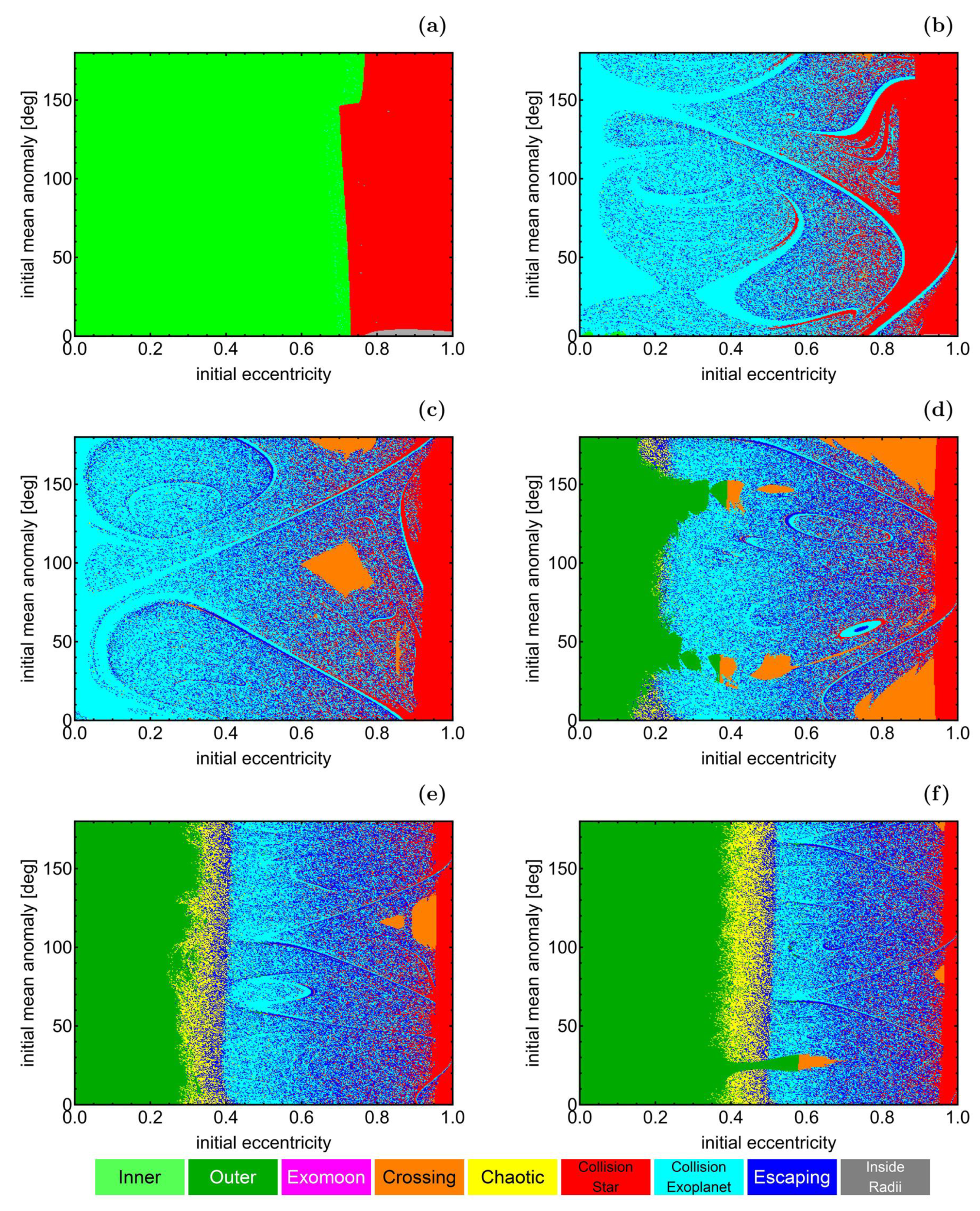
The initial configuration of the bodies with masses $m_2$ and $m_3$ is of paramount importance and is determined by the initial values $M_2$ and $M_3$ of their mean anomalies. We provide basin diagrams on the $(a_3,M_3)$ plane in Figure 4a–f and Figure 5a–f to illustrate the results for different initial eccentricity values of $e_3$, assuming $M_2=0$. Furthermore, Figure 4 corresponds to $m_2=5$ $M_J$ and Figure 5 to $m_2=70$ $M_J$.

When we consider the scenario of a transiting super-Jupiter with a mass of $m_2=5$ $M_J$, several observations can be made from Figure 4a–f as the eccentricity $e_3$ increases:

• The number of inner-type trajectories decreases significantly. When $e_3=0.8$, these trajectories result in immediate collisions with the host star.
• The area of stability islands associated with outer-type trajectories appears to decrease. However, in reality, these stability islands shift to greater distances from the center.
• The number of crossing-type trajectories increases, and we observe the emergence of additional stability islands between the inner and outer basins.
• Our computations indicate no presence of exomoon-type trajectories whatsoever. This supports our previously published findings in Moneer et al. [15], where we demonstrated that exomoon-type orbits are only possible when $M_2=M_3=0$ or $M_2=M_3=180°$.
• Within the zone that lies between the stability islands representing inner and outer-type trajectories, there exists a distinct region characterized by an intricate mixture of trajectories that either escape or collide.

In Figure 4, we observed the orbital properties of a super-Jupiter, while in Figure 5a–f, we focus on a brown dwarf with a mass equal to 70 $M_J$. A significant difference is evident in the behavior of the Earth-size exoplanet’s orbital properties between the two cases. The stability islands of the inner and outer-type trajectories exhibit similar behavior as shown in Figure 4. However, there are substantial changes in the orbital structure within the areas between these stability islands. Specifically, in the case of low values of $m_2$, the once “chaotic” regions now exhibit clearly defined basins of escape and collision. This phenomenon gives rise to the formation of complex spiral structures. Additionally, the presence of crossing-type trajectories is significantly diminished in this case, in contrast to the abundance of stability islands observed when $m_2$ was 5 $M_J$, which are now nearly absent.

4.3. The $(e_3,M_3)$ Survey

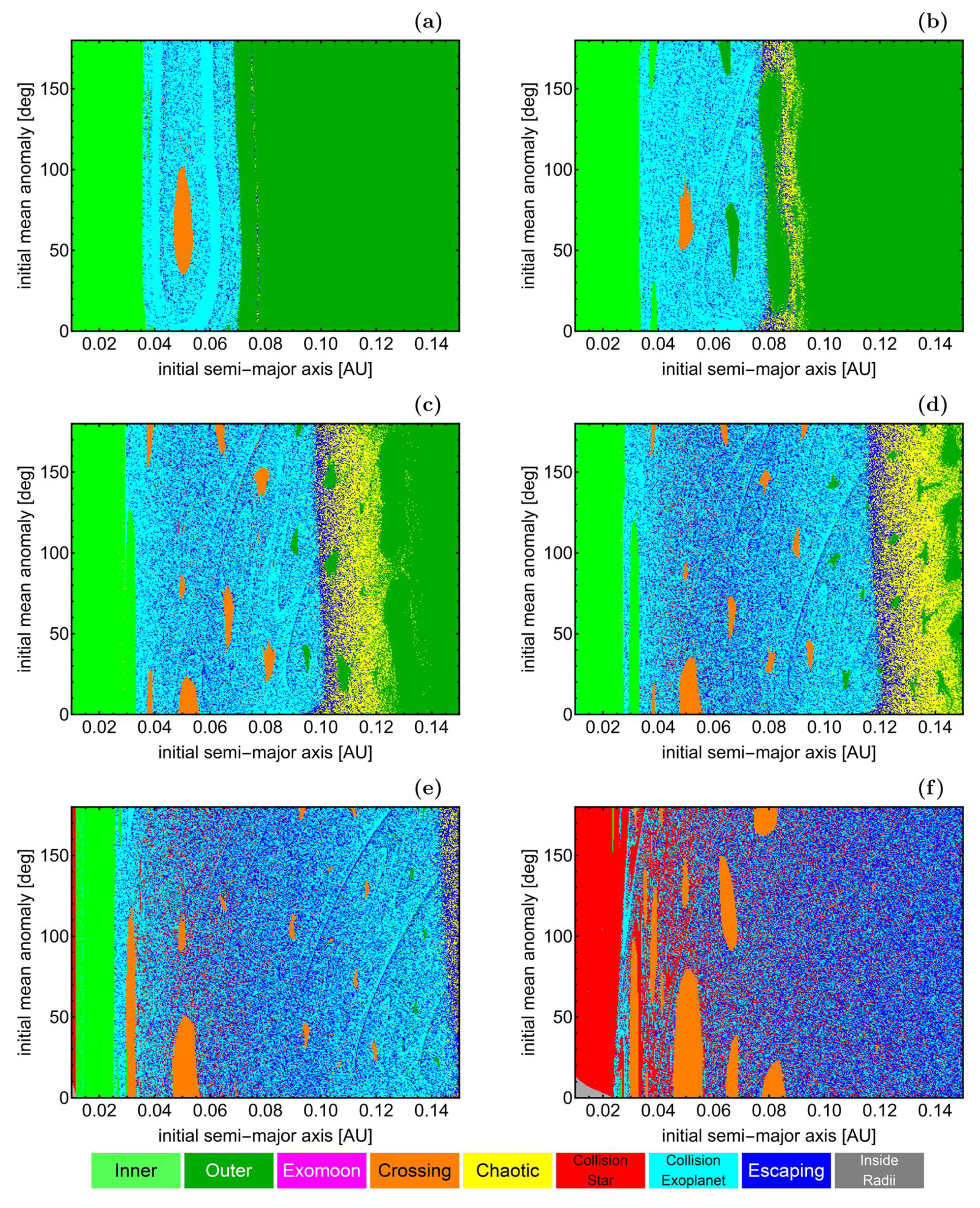
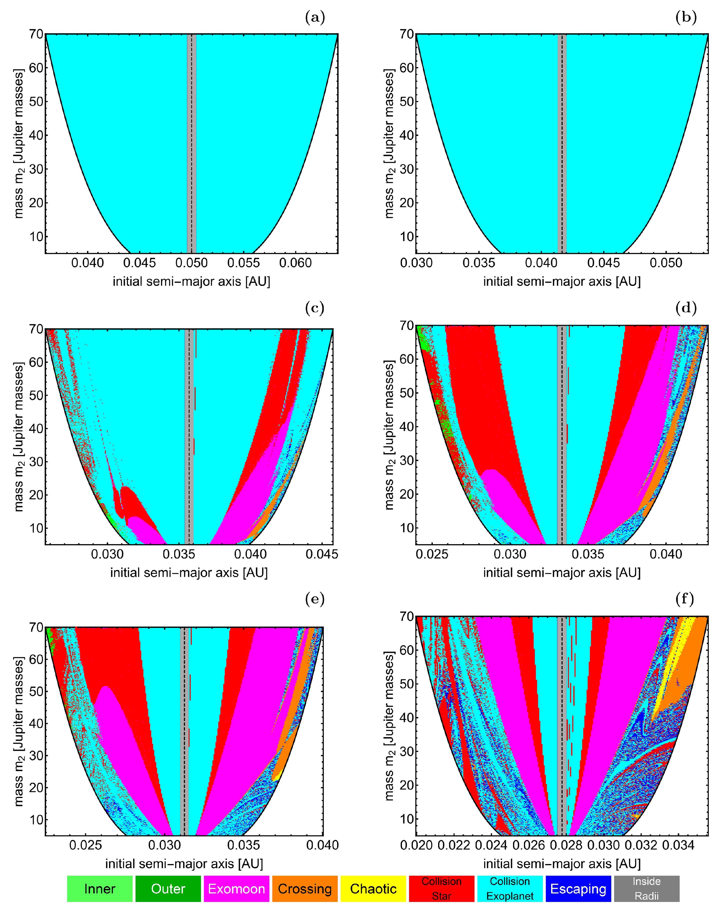
In order to explore the orbital properties of the system’s phase space, another approach is to analyze the $(e_3,M_3)$ plane for various values of the initial semi-major axis $a_3$. Figure 6a–f and Figure 7a–f present the basins diagrams classifying the initial conditions of Earth-size exoplanets for $m_2$ equal to 5 and 70 $M_J$, respectively.

For a super-Jupiter with a mass of $m_2=5$ $M_J$, Figure 6 reveals the following:

• For relatively low values of the initial semi-major axis (panel (a)), most of the phase space is occupied by initial conditions corresponding to inner-type regular trajectories.
• As $a_3$ increases within intermediate values $(0.04<a_3<0.06)$, escaping and collision trajectories dominate. Beyond $a_3>0.06$, outer-type trajectories begin to emerge while the occurrence of escaping and collision orbits decreases.
• When eccentricity values are relatively high $(e_3>0.6)$, both inner and outer orbits transition into escaping or collisional trajectories, accompanied by the emergence of stability islands for crossing-type trajectories.
• Once again, the regions of the phase space occupied by escaping and collisional trajectories exhibit high unpredictability due to the “chaotic” mixture of initial conditions.
• For extremely high initial eccentricity values $(e_3>0.95)$, nearly all initial conditions result in trajectories that collide with the host star, regardless of the specific initial value of the mean anomaly $M_3$.

For the case of the transiting brown dwarf with $m_2=70$ $M_J$, we see in Figure 7a–f that things are very similar to what we have seen earlier in Figure 4 and Figure 5. Indeed, the main difference that occurs due to the substantial increase in the mass is the orbital structure of the regions occupied by escaping and collisional trajectories. Specifically, we see that most of these regions contain well-defined basins of escape and collision, while the “chaotic” mixture of initial conditions where we cannot predict the final state of the Earth-size exoplanet has been heavily reduced. Once more, these well-formed basins form complicated spiral structures that extend to all the available phase space of the system.

4.4. The $(a_3,m_2)$ Survey

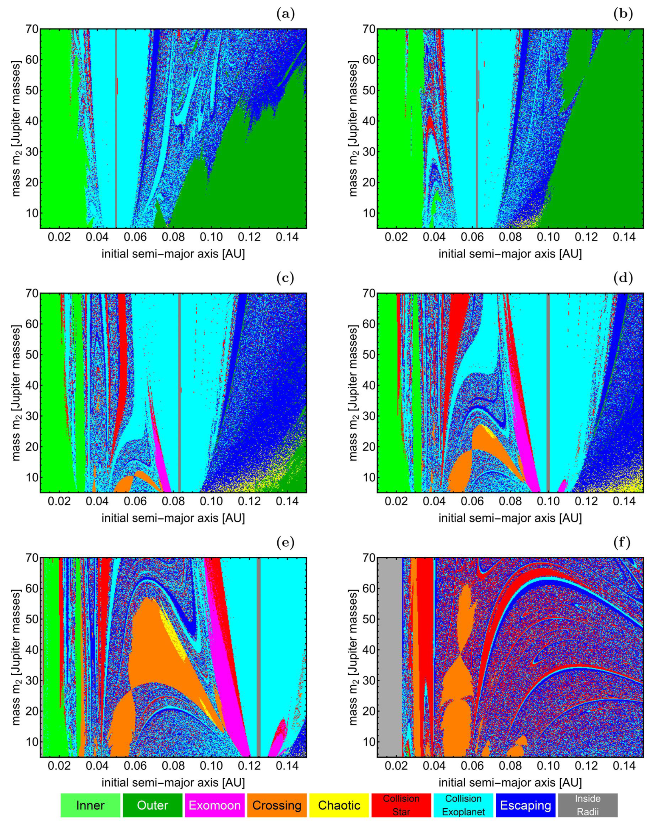
So far, we have discussed the orbital properties of the system for specific values of the mass $m_2$ of the transiting body. However, we can extract additional interesting information by scanning a continuous spectrum of values for $m_2$. In order to accomplish this, we present the classification of the initial conditions of the trajectories on the $(a_3,m_2)$ plane for different values of the initial eccentricity $e_3$ in Figure 8a–f.

On the $(a_3,m_2)$ plane, we observe the following changes as the value of $m_2$ increases:

• For low initial values of the eccentricity $(e_3<0.5)$, the areas occupied by inner and outer-type regular trajectories are reduced, allowing more escaping and collisional trajectories to occur.
• For intermediate initial values of the eccentricity $(0.5<e_3<0.9)$, we observe the presence of crossing-type trajectories. Our computations suggest that the proportion of these orbits increases with higher values of $m_2$.
• The same pattern described above for crossing-type trajectories also applies to exomoon-type trajectories.
• For high initial values of the eccentricity $(e_3\ge 0.8)$, the phase space is predominantly occupied by initial conditions leading to escaping and collisional trajectories.
• These basin diagrams provide a clearer representation of how the fractality of the phase space decreases as the mass $m_2$ increases, due to the emergence of well-defined escape basins (see panel (f) of Figure 8).

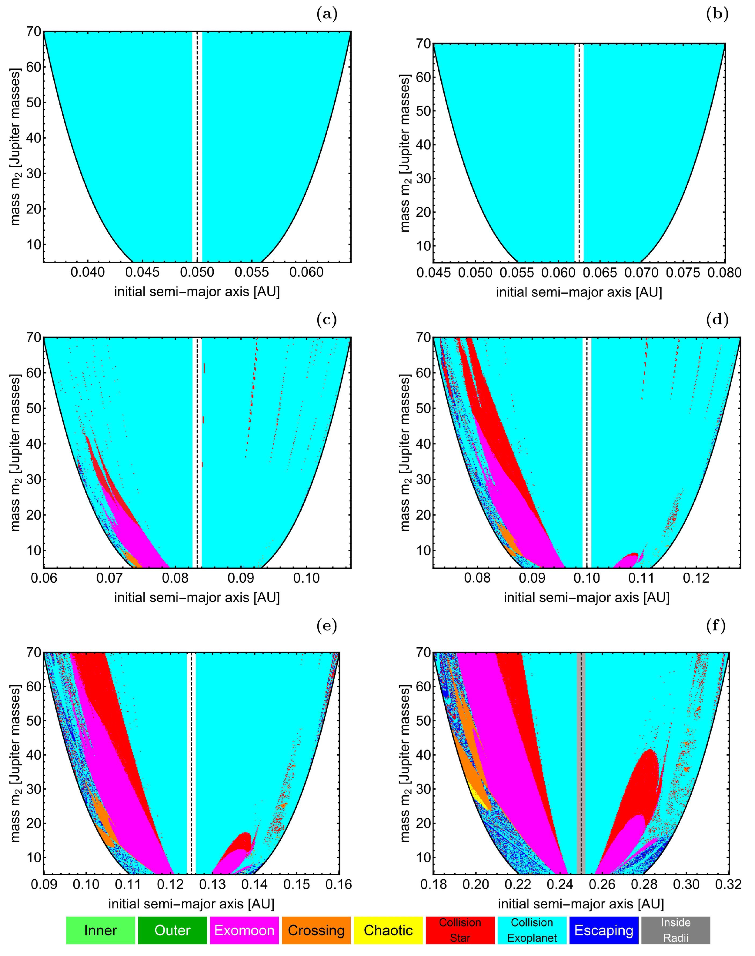
4.5. Searching for Exomoons

The cases where an Earth-size exoplanet acts as an exomoon of the transiting body with mass $m_2$ are of particular interest. In [15], we argued that all trajectories classified as exomoon-type orbits remain well within the Hill sphere of the transiting body throughout the numerical integration. To prove this, we extended the integration time of all exomoon-type orbits to ${10}^5$ orbital periods to observe their stability and whether they eventually lead to escape or collision after a considerable period of time. Our calculations strongly suggested that all trajectories remain inside the Hill sphere even after ${10}^5$ orbital periods. Therefore, we can confidently conclude that these are true exomoon-type orbits, not quasi-satellite orbits.

In our previous analysis [15], we also discovered that exomoon-type orbits are only possible when the initial values of the mean anomalies of the transiting body and the Earth-size exoplanet are the same (either 0 or 180°). Hence, in Figure 9a–f and Figure 10a–f, we present the classification of initial conditions for trajectories inside the Hill sphere of the transiting body $m_2$. Each panel corresponds to a different initial value of the eccentricity $e_3$. For Figure 9 and Figure 10, we set $M_2=M_3=0$ and $M_2=M_3=180°$, respectively. In Figure 9, the vertical dashed line indicates the perihelion distance $(a_3(1-e_3)=0.05)$, while in Figure 10, it represents the aphelion distance $(a_3(1+e_3)=0.05)$.

In both cases (regarding the initial values of the mean anomalies), it can be observed that, for low values of the initial eccentricity $(e_3\le 0.2)$, the Hill sphere is entirely occupied by initial conditions that result in a collision with the transiting body $m_2$. As the initial eccentricity increases $(e_3>0.2)$, initial conditions of exomoon-type orbits start to appear, and their quantity increases with a higher value of eccentricity $e_3$. Two phenomena of interest can be noted: (i) the presence of exomoon-type orbits seems to be more pronounced when studying them along the aphelion distance, and (ii) for initial eccentricity values $(e_3\ge 0.8)$, the Hill sphere contains a diverse combination of different types of initial conditions of trajectories (particularly along the aphelion distance). In general terms, it can be argued that increasing the mass of the transiting body enhances the presence of exomoon-type trajectories.

It should be stressed that if the initial conditions inside the Hill sphere correspond to stable regular motion, it does not necessarily mean that they are exomoon-type trajectories. In fact, within the basin diagrams of both Figure 9a–f and Figure 10a–f, there exist initial conditions of regular bounded orbits that are crossing-type trajectories.

4.6. Degree of Fractality

Before concluding our analysis, we would like to present some quantitative results regarding the influence of the mass $m_2$ of the transiting body on the degree of fractality in the system’s phase space. To measure this, we employ the fractal or uncertainty dimension $D_0$ [26]. The uncertainty dimension quantifies the degree of irregularity or self-similarity in a set of data or geometric shapes. It is calculated using the box-counting method

$$D_0=\underset{\epsilon \to 0}{lim}\frac{log\left(N\right(\epsilon \left)\right)}{log(1/\epsilon )},$$

(3)

where $N\left(\epsilon \right)$ is the minimum number of boxes of size $\epsilon$ needed to cover the set, and $\epsilon$ is the size of the boxes used for covering the set. It is worth noting that, when computing the fractal dimension of a two-dimensional basin diagram, if $D_0\to 1$, it suggests minimal fractality, whereas if $D_0\to 2$, it indicates complete fractality of the corresponding basin diagram.

We computed the fractal dimension for the basin diagrams shown in Figure 4, Figure 5, Figure 6 and Figure 7. For the six panels of Figure 4 (corresponding to $m_2=5$ $M_J$), the resulting values of $D_0$ are 1.23, 1.31, 1.62, 1.78, 1.82, and 1.78, respectively. Similarly, for the six panels of Figure 5 (corresponding to $m_2=70$ $M_J$), the resulting values of $D_0$ are 1.27, 1.22, 1.48, 1.61, 1.69, and 1.72, respectively. By following the same methodology, we obtained the values of $D_0$ for the six panels of Figure 6 (corresponding to $m_2=5$ $M_J$) as 1.03, 1.68, 1.72, 1.57, 1.44, and 1.32, respectively. Similarly, for the six panels of Figure 7 (corresponding to $m_2=70$ $M_J$), the resulting values of $D_0$ are 1.09, 1.42, 1.37, 1.45, 1.39, and 1.26, respectively.

It is clear that, in almost all cases, the value of the fractal dimension $D_0$ is lower when the mass of the transiting body is higher. Therefore, we can argue that systems with massive transiting bodies exhibit a significantly lower degree of unpredictability compared to systems with less massive transiting bodies.

5. Discussion

In this research work, we investigated the orbital dynamics of an exosystem consisting of a host star, a transiting body, and an Earth-size exoplanet using numerical methods and the theory of the generalized three-body problem. The astrophysical nature of the transiting body varied between a super-Jupiter or a brown dwarf, depending on its mass. By systematically and thoroughly classifying the available phase space, we determined the final states of the Earth-size exoplanet. This classification allowed us to distinguish between the bounded, escaping, and collisional motions of the Earth-size exoplanet. Additionally, for cases of ordered (regular) motion, we further classified the corresponding initial conditions into subcategories based on the geometry of the trajectories. These bounded regular trajectories are of great importance as they reveal phase space regions where the motion of the Earth-size exoplanet can be dynamically stable. Of particular interest was the detection of initial conditions where the Earth-size exoplanet acts as an exomoon of the transiting body, always remaining within its Hill radius.

The following list summarizes the most important findings of our survey:

• Generally, as the mass of the transiting body increases, the presence of inner, outer, and crossing-type trajectories weakens. However, exomoon-type trajectories seem to be enhanced by the increased mass of the transiting body. It is important to note that the exomoon-type trajectories move further from the center as the mass $m_2$ increases.
• The number of both escaping and collision types of trajectories increases as the mass of the transiting body increases.
• We observed that, in cases with low values of $m_2$ (corresponding to cases where the transiting body is a super-Jupiter), the phase space exhibits a high degree of fractality due to a chaotic mixture of escaping and collisional trajectories. Conversely, when the value of $m_2$ is relatively high (corresponding to cases where the transiting body is a brown dwarf), the degree of fractality in the phase space significantly reduces due to the emergence of well-defined basins of escape and collision.
• The majority of stable motion corresponds to simple loop orbits. However, for low values of $m_2$, there are numerous stability islands corresponding to higher secondary resonant crossing-type trajectories. This type of orbit primarily appears with high initial eccentricities of the Earth-size exoplanet.
• Our analysis of the phase space inside the Hill sphere around the transiting body suggests that for low initial eccentricities $e_3$, the entire phase space consists of initial conditions that result in collision with the transiting body. However, as the value of $e_3$ increases, the structure of the phase space changes, and stability islands corresponding to exomoon-type trajectories appear on both sides along the perihelion and aphelion distances.

Judging by the positive results of our analysis, we plan to expand our survey by considering specific exosystems (containing a host star and a transiting body) and focus our attention on the exploration of possible exomoon-type orbits around the transiting bodies.

References

- Howard, A.W.; Marcy, G.W.; Bryson, S.T.; Jenkins, J.M.; Rowe, J.F.; Batalha, N.M.; Borucki, W.J.; Koch, D.G.; Dunham, E.W.; Gautier, T.N.; et al. Planet occurrence within 0.25 AU of solar-type stars from Kepler. Astrophys. J. Suppl. Ser. 2012, 201, 15. [Google Scholar] [CrossRef]
- Ricker, G.R.; Winn, J.N.; Vanderspek, R.; Latham, D.W.; Bakos, G.Á.; Bean, J.L.; Berta-Thompson, Z.K.; Brown, T.M.; Buchhave, L.; Butler, N.R.; et al. Transiting exoplanet survey satellite. J. Astron. Telesc. Instrum. Syst. 2015, 1, 014003. [Google Scholar] [CrossRef]
- Winn, J.N.; Fabrycky, D.C. The occurrence and architecture of exoplanetary systems. Annu. Rev. Astron. Astrophys. 2015, 53, 409. [Google Scholar] [CrossRef]
- Borucki, W.J. Kepler: A brief discussion of the mission and exoplanet results. Proc. Am. Philos. Soc. 2017, 161, 38. [Google Scholar]
- Inayoshi, K.; Onoue, M.; Sugahara, Y.; Inoue, A.K.; Ho, L.C. The Age of Discovery with the James Webb Space Telescope: Excavating the Spectral Signatures of the First Massive Black Holes. Astrophys. J. Lett. 2022, 931, L25. [Google Scholar] [CrossRef]
- Gardner, J.P.; Mather, J.C.; Clampin, M.; Doyon, R.; Greenhouse, M.A.; Hammel, H.B.; Hutchings, J.B.; Jakobsen, P.; Lilly, S.J.; Long, K.S.; et al. The james webb space telescope. Space Sci. Rev. 2006, 123, 485–606. [Google Scholar] [CrossRef]
- Pepe, F.; Ehrenreich, D.; Meyer, M.R. Instrumentation for the detection and characterization of exoplanets. Nature 2014, 513, 358. [Google Scholar] [CrossRef]
- Maxted, P.F.L.; Ehrenreich, D.; Wilson, T.G.; Alibert, Y.; Cameron, A.C.; Hoyer, S.; Sousa, S.G.; Olofsson, G.; Bekkelien, A.; Deline, A.; et al. Analysis of Early Science observations with the CHaracterising ExOPlanets Satellite (CHEOPS) using pycheops. Mon. Not. R. Astron. Soc. 2022, 514, 77–104. [Google Scholar] [CrossRef]
- Birkmann, S.M.; Ferruit, P.; Giardino, G.; Nielsen, L.D.; Muñoz, A.G.; Kendrew, S.; Rauscher, B.J.; Beck, T.L.; Keyes, C.; Valenti, J.A.; et al. The near-infrared spectrograph (nirspec) on the james webb space telescope-iv. capabilities and predicted performance for exoplanet characterization. Astron. Astrophys. 2022, 661, A83. [Google Scholar] [CrossRef]
- Domingos, R.C.; Winter, O.C.; Yokoyama, T. Stable satellites around extrasolar giant planets. Mon. Not. R. Astron. Soc. 2006, 373, 1227–1234. [Google Scholar] [CrossRef]
- Antoniadou, K.I.; Voyatzis, G. Orbital stability of coplanar two-planet exosystems with high eccentricities. Mon. Not. R. Astron. Soc. 2016, 461, 3822–3834. [Google Scholar] [CrossRef]
- Antoniadou, K.I.; Voyatzis, G. Periodic orbits in the 1:2:3 resonant chain and their impact on the orbital dynamics of the Kepler-51 planetary system. Astron. Astrophys. 2022, 661, A62. [Google Scholar] [CrossRef]
- Kane, S.R.; Raymond, S.N. Orbital dynamics of multi-planet systems with eccentricity diversity. Astrophys. J. 2014, 784, 104. [Google Scholar] [CrossRef]
- Davies, M.B.; Adams, F.C.; Armitage, P.; Chambers, J.; Ford, E.; Morbidelli, A.; Raymond, S.N.; Veras, D. The Long-Term Dynamical Evolution of Planetary Systems; University of Arizona Press: Tucson, AZ, USA, 2013. [Google Scholar]
- Moneer, E.M.; Dubeibe, F.L.; Allawi, Y.M.; Alanazi, M.M.; Hinse, T.C.; Zotos, E.E. Classification of Trajectories in a Two-planet Exosystem Using the Generalized Three-body Problem. Astrophys. J. 2023, 952, 104. [Google Scholar] [CrossRef]
- Laughlin, G. Handbook of Exoplanets; Springer International Publishing AG, part of Springer Nature: Berlin/Heidelberg, Germany, 2018. [Google Scholar]
- Hatzes, A.P.; Rauer, H. A definition for giant planets based on the mass–density relationship. Astrophys. J. Lett. 2015, 810, L25. [Google Scholar] [CrossRef]
- Press, H.P.; Teukolsky, S.A.; Vetterling, W.T.; Flannery, B.P. Numerical Recipes in FORTRAN 77, 2nd ed.; Cambridge University Press: Cambridge, MA, USA, 1992. [Google Scholar]
- Zotos, E.E.; Érdi, B.; Saeed, T.; Alhodaly, M.S. Orbit classification in exoplanetary systems. Astron. Astrophys. 2020, 634, A60. [Google Scholar] [CrossRef]
- Skokos, C. Alignment indices: A new, simple method for determining the ordered or chaotic nature of orbits. J. Phys. A 2001, 34, 10029. [Google Scholar] [CrossRef]
- Skokos, C.; Antonopoulos, C.; Bountis, T.C.; Vrahatis, M.N. How does the Smaller Alignment Index (SALI) distinguish order from chaos? Prog. Theor. Phys. Suppl. 2003, 150, 439–443. [Google Scholar] [CrossRef]
- Skokos, C.; Antonopoulos, C.; Bountis, T.C.; Vrahatis, M.N. Detecting order and chaos in Hamiltonian systems by the SALI method. J. Phys. A Math. Gen. 2004, 37, 6269. [Google Scholar] [CrossRef]
- Zotos, E.E.; Veras, D.; Saeed, T.; Darriba, L.A. Short-term stability of particles in the WD J0914+ 1914 white dwarf planetary system. Mon. Not. R. Astron. Soc. 2020, 497, 5171–5181. [Google Scholar] [CrossRef]
- Nagler, J. Crash test for the Copenhagen problem. Phys. Rev. E 2004, 69, 066218. [Google Scholar] [CrossRef]
- Nagler, J. Crash test for the restricted three-body problem. Phys. Rev. E 2005, 71, 026227. [Google Scholar] [CrossRef]
- Ott, E. Chaos in Dynamical Systems; Cambridge University Press: Cambridge, MA, USA, 1993. [Google Scholar]
Figure 1.
Distribution of masses and radii for currently known super-Jupiter exoplanets. The mean mass and radius are represented by a five-pointed red star. For further information, please refer to https://exoplanetarchive.ipac.caltech.edu/ (accessed on 5 May 2023).
Figure 2.
Schematic representations illustrating characteristic examples of orbit classification for regular orbits of , which refers to an exoplanet of Earth-size. Each panel provides a depiction of distinct orbit types, including: (a) a circumstellar orbit, (b) a circumbinary orbit, (c) a circumplanetary orbit, and (d) an intersecting orbit.
Figure 3.
Classification maps for (Earth-size exoplanet), using different values of . The dashed black lines denote a fixed radius measured from (star) in which the aphelion and perihelion distances are equal to 0.05 AU. The mass of the transiting body changes as follows: (a): = 5 , (b): = 15 , (c): = 30 , (d): = 45 , (e): = 60 , and (f): = 70 .
Figure 4.
Classification maps for (Earth-size exoplanet), using different values of and also when . The initial eccentricity changes as follows: (a): = 0, (b): = 0.2, (c): = 0.4, (d): = 0.5, (e): = 0.6, and (f): = 0.8.
Figure 5.
Figure 6.
Classification maps for (Earth-size exoplanet), using different values of and also when . The initial value (in AU) of the semi-major axis changes as follows: (a): = 0.02, (b): = 0.04, (c): = 0.06, (d): = 0.08, (e): = 0.10, and (f): = 0.12.
Figure 7.
Figure 8.
Classification maps for (Earth-size exoplanet), using different values of . The initial value of the eccentricity changes as follows: (a): = 0, (b): = 0.2, (c): = 0.4, (d): = 0.5, (e): = 0.6, and (f): = 0.8.
Figure 9.
Classification maps for (Earth-size exoplanet), using different values of , when . All the initial conditions are inside the Hill sphere of the transiting body with mass . The initial value of the eccentricity changes as follows: (a): = 0, (b): = 0.2, (c): = 0.4, (d): = 0.5, (e): = 0.6, and (f): = 0.8.
Figure 10.
Disclaimer/Publisher’s Note: The statements, opinions and data contained in all publications are solely those of the individual author(s) and contributor(s) and not of MDPI and/or the editor(s). MDPI and/or the editor(s) disclaim responsibility for any injury to people or property resulting from any ideas, methods, instructions or products referred to in the content. |
© 2024 by the authors. Licensee MDPI, Basel, Switzerland. This article is an open access article distributed under the terms and conditions of the Creative Commons Attribution (CC BY) license (https://creativecommons.org/licenses/by/4.0/).
Share and Cite
MDPI and ACS Style
Zotos, E.E.; Moneer, E.M.; Hinse, T.C. Classification of Planetary Motion around Super-Jupiters and Brown Dwarfs. Universe 2024, 10, 138. https://doi.org/10.3390/universe10030138
AMA Style
Zotos EE, Moneer EM, Hinse TC. Classification of Planetary Motion around Super-Jupiters and Brown Dwarfs. Universe. 2024; 10(3):138. https://doi.org/10.3390/universe10030138
Chicago/Turabian StyleZotos, Euaggelos E., Eman M. Moneer, and Tobias C. Hinse. 2024. "Classification of Planetary Motion around Super-Jupiters and Brown Dwarfs" Universe 10, no. 3: 138. https://doi.org/10.3390/universe10030138
Note that from the first issue of 2016, this journal uses article numbers instead of page numbers. See further details here.